In this work a perturbative linear response analysis is performed for the time evolution of the “quasi-conserved” charge of a scalar field. One can find two regimes, one follows exponential damping, where the damping rate is shown to come from quantum Boltzmann equations. The other regime (coming from multiparticle cuts and products of them) decays as power law. The most important, non-oscillating contribution in our model comes from a 4-particle intermediate state and decays as $1/t^{3}$. These results may have relevance for instance in the context of lepton number violation in the Early Universe.

1 Introduction

Recently, in a series of papers [1], Joichi, Matsumoto and Yoshimura analyzed the effects of the quantum-improved Boltzmann equations. The authors developed a model of unstable particles and found that their Boltzmann equations generate a non-exponentially-suppressed equilibrium distribution function for heavy particles at low temperatures. This deviation from the standard picture was due to cut contributions far from the quasi-particle pole. These works were later criticized by several authors [2, 3, 4], their main point being that the definition of particle number is delicate for unstable particles. Redefining particle number may change the coefficient of the non-exponential term [3], or completely cancel it [2]. In [4] the authors argued that the naive definition needs renormalization in perturbation theory and proposed a non-perturbative definition for the number density.

Non-quasi-particle properties of the quantum fields may change also the time evolution of the physical observables, as was also emphasized in [1]. The same phenomenon was found also in the time evolution of bosonic condensates [5, 6]. In these latter cases power-law decay was shown up even in the linear response theory.

In this paper we use linear response perturbation theory to investigate the long-time behavior of composite operators. As a specific example we consider the “quasi-conserved” charge of a scalar field. In this way we cannot address the equilibrium state; still, it is a physical scheme at which practically all systems must arrive after long time evolution. The numerical advantage is that all expectation values are defined in equilibrium, so that they can, in principle, be calculated without additional approximation. It is very important that the different contributions are additive, which makes it possible to identify different physical effects without entangling them.

In fact there is a close analogy in the formalism describing the time evolution of the field condensates [5, 6] and the scalar charge operators; the details will be explained in the paper. In linear response theory the field condensates are proportional to the retarded Green’s function; in the case of the charge $Q$ we have instead $QF$ retarded Green’s function (with arbitrary $F$). The discontinuity of the retarded propagator for free case is a delta function concentrated on the mass shell. In the free theory $Q$ is conserved, thus the discontinuity of $QF$ retarded Green’s function is $\sim\delta(k_{0})$ – this is the “mass shell” of the $QF$ spectral function. In the interacting case, at small coupling, the mass shell still represents quasi-particles. In a similar way the charge, although not conserved, characterizes the system well. In analogy to quasi-particles we call it quasi-conserved charge.

The shift of the mass shell is not a perturbative effect. Indeed, when we calculate the propagator in perturbation theory we find IR divergences on the mass shell. One uses Schwinger–Dyson equations to resum these divergences, and a Breit–Wigner approximation to describe the shift of the mass shell. The same phenomenon appears also in the $QF$ propagator: the shift of the “mass shell” causes IR divergences in perturbation theory at $k_{0}=0$. In coordinate space these divergences are manifested as secular terms. These, as was shown by [7], can be resummed to quantum Boltzmann equations. In momentum space the same phenomenon shows up as pinch singularities [8, 9, 10, 11]. In order to resum them we have to consider ladder diagrams [12, 13, 14, 15, 16], which we will show to result in Kadanoff–Baym equations. These are, at lowest order [17], the usual Boltzmann equations. Thus the analogy of the Schwinger–Dyson resummation in Breit–Wigner approximation is the use of Boltzmann equations in the composite operator case.

The analogy, however, extends even more. In the propagator we find, apart from the broadened mass shell, other structures as well. Most important are the analytic defects (e.g. multiparticle cuts), which play an important role in the long-time evolution, as they give power-law decay [1, 5, 6]. These are not related to the broadening, and they are perturbative in the massive case. We find similar defects in the $QF$ propagator, giving power-law decay at large times, which are independent of the Boltzmann equations.

This paper is structured as follows. In Section 2 we work out how initial conditions can be taken into account in linear response theory and what kind of long-time behavior can be expected. It has two ingredients: a pole contribution, which yields exponential damping, and a power-law correction coming from other analytic defects (such as cuts). In Section 3 the first contribution is considered and it is shown that this comes from the quantum Boltzmann equations (Kadanoff–Baym equations). In Section 4 the off-shell analytic defects are investigated. Multiparticle cuts give a power-law, oscillating time dependence. It is shown, however, that they can be combined even at the linear response level giving non-oscillating time dependence. In Section 5 we summarize our findings.

2 Long-time behavior in linear response theory

2.1 The model

Inspired by the discussion about the particle number, we choose a well-measurable observable: the charge of a bosonic field (cf. [2]). The Lagrangian

$${\cal L}=-\Psi^{\dagger}(\partial^{2}+m_{\Psi}^{2})\Psi-\chi^{\dagger}(\partial^{2}+m_{\chi}^{2})\chi-\frac{1}{2}\Phi(\partial^{2}+m_{\Phi}^{2})\Phi-h\Phi(\Psi^{\dagger}\chi+\chi^{\dagger}\Psi)$$ (1)

contains a heavy charged $\Psi$ particle (with mass $m_{\Psi}$) and a light charged $\chi$ particle (with mass $m_{\chi}$) coupled through a Yukawa term with a scalar $\Phi$ (with mass $m_{\Phi}$).

Without the Yukawa term, the U(1) phase symmetry would be perfect, and the currents

$$J^{\Psi}_{\mu}=\Psi^{\dagger}\,i\mathop{\mbox{$\partial$\raisebox{8.00003pt}{$\scriptstyle\leftrightarrow$} }}\Psi\quad\textrm{and}\quad J^{\chi}_{\mu}=\chi^{\dagger}\,i\mathop{\mbox{$\partial$\raisebox{8.00003pt}{$\scriptstyle\leftrightarrow$} }}\chi$$ (2)

would be conserved quantities. For $h\neq 0$ they are not conserved

$$\partial J^{\Psi}=ih\Phi(\chi^{\dagger}\Psi-\Psi^{\dagger}\chi),\qquad\partial J^{\chi}=ih\Phi(\Psi^{\dagger}\chi-\chi^{\dagger}\Psi),$$ (3)

only their sum is. Our final goal is to describe the time evolution of the charge of $\Psi$ and $\chi$

$$Q^{\Psi}(t)=\left\langle{\hat{Q}^{\Psi}(t)}\right\rangle=\mathop{\textrm{Tr}}\hat{\rho}Q^{\Psi}(t),\qquad\hat{Q}^{\Psi}(t)=\int\!d^{3}{\bf x}\,J^{\Psi}_{0}({\bf x},t),$$ (4)

and similarly for $\chi$, where $\hat{\rho}$ is the initial density matrix. In order to avoid complications with the chemical potential, we assume that the total charge is zero.

2.2 Linear response theory

Tracing the time evolution, starting from a non-equilibrium density matrix, is usually a hard task [18]. Here we follow a way where we construct the initial state from equilibrium by acting on the system with a time-dependent external force – after all this is the way one acts in a real experiment. At $t=-\infty$ we start from equilibrium, then we prepare the initial conditions by changing $H\to H+H_{ext}(t)$ for times $-\infty<t<0$, finally we turn off the external force and start to measure for $0<t<\infty$.

This picture can be formulated in path integral representation, since at $t=-\infty$ we have equilibrium ensemble. For an observable $O(x)$

$$\left\langle{O(x)}\right\rangle=\frac{1}{Z}\int\limits_{KMS}\!\!O(x)\,e^{iS-i\int_{c}\zeta F},$$ (5)

where $\int_{KMS}$ denotes path integration where the paths are subject to KMS conditions along the applied Keldysh contour $c$. The external force is $F$ and its explicitly time-dependent amplitude is denoted by $\zeta(t)$ (here $t$ is the real time, not the contour time variable).

By the end of a realistic time evolution, we deviate only slightly from equilibrium; therefore we expect that the corresponding state can be produced using a weak force. That means that in this case we can use linear response theory. If in equilibrium $\left\langle{O}\right\rangle_{eq}=0$ then we have

$$\left\langle{O(x)}\right\rangle=-i\int d^{4}x^{\prime}\,\Theta(t-t^{\prime})\left\langle{[O(x),F(x^{\prime})]}\right\rangle_{eq}\zeta(x^{\prime}).$$ (6)

Here the expectation value of the commutator has to be taken in equilibrium, and therefore it is a function of $x-x^{\prime}$. We denote

$$i{\cal G}_{R}^{(OF)}(x)=\Theta(t)\left\langle{[O(x),F(0)]}\right\rangle_{eq},\qquad\varrho^{(OF)}(x)=\left\langle{[O(x),F(0)]}\right\rangle_{eq};$$ (7)

note that in Fourier space $\varrho^{(OF)}(k)=i\mathop{\textrm{Disc}}\limits_{k_{0}}{\cal G}_{R}^{(OF)}(k)$.

For our concrete observable,

$$Q(k_{0})=\left\langle{J_{0}(k_{0},{\bf k}=0)}\right\rangle={\cal G}_{R}^{(J_{0}F)}(k)\zeta(k)\bigr{|}_{{\bf k}=0}.$$ (8)

This is very similar, in spirit, to the usual Kubo formulae [19], the only difference being that now the external force is not fixed. In principle we can imagine a lot of possible choices (e.g. a plausible one $F\sim H_{I}$ where $H_{I}$ is the interaction Hamiltonian); what is only important is that it should create a net $Q(0)$, i.e. $[\hat{Q},F]\neq 0$.

Having the formal result in hand, there is still a question of how to characterize the process and how to compute the specific numbers. In general we expect that, close to $t=0$ when the external force was switched off, the time evolution contains a lot of transients. This is reflected also in the fact that $Q(t)$ depends strongly on the choice of $F$. Only after a long time do we expect that the time dependence is independent of the initial conditions. Concentrating on this region we now examine the long-time behavior of an expression like (8).

2.3 Long-time behavior: the general case

This analysis follows closely the one of Refs. [5, 6], including also the $\zeta$ dependence. We examine the long-time behavior of

$$f(t)=\int\!\frac{dk_{0}}{2\pi}\,e^{-ik_{0}t}\,{\cal G}_{R}(k_{0})\zeta(k_{0}),$$ (9)

where ${\cal G}_{R}$ is a general retarded Green’s function, $\zeta$ is the amplitude of the external force. We assume that the analytic defects of $\zeta(k_{0})$ are on the upper half-plane and the ones of $G_{R}$ are along the real axis. Then, taking into account that using retarded Green’s functions means that we have to use a contour that runs slightly above the real axis in $k_{0}$, we can extend the integration region for $t>0$ as is shown in Fig. 1a (the semi-circle at infinity gives zero contribution).

Figure 1: Transformation of the integration contours.

Under our assumptions the closed circle on the lower half-plane gives zero, while the rest picks up the discontinuity of $G_{R}$

$$f(t)=\int\!\frac{dk_{0}}{2\pi i}\,e^{-ik_{0}t}\,\varrho(k_{0})\zeta(k_{0}).$$ (10)

The spectral function $\varrho$ may contain poles or discontinuities in derivatives of some order (ie. thresholds), but these defects form a discrete set. In between, the spectral function is analytic. We transform the piecewise analytic parts further. For a single interval running from $-\infty\to a$:

$$\int\limits_{-\infty}^{a}\frac{dk_{0}}{2\pi i}\,e^{-ik_{0}t}\,\varrho(k_{0})\zeta(k_{0})=e^{-iat}\int\limits_{-\infty}^{0}\frac{dk_{0}}{2\pi i}\,e^{-ik_{0}t}\,\varrho(k_{0}+a)\zeta(k_{0}+a).$$ (11)

Now we add the zero contribution of a quarter circle at infinity and a contour running up and down on the negative imaginary axis as shown by Fig. 1b. The closed loop picks up the contributions of the poles inside; in the rest we change variables $ik_{0}\to y$ and write

$$\mathop{\textrm{Res}}\limits_{\omega\in\textrm{\scriptsize loop}}\left[\varrho(\omega)\zeta(\omega)e^{-i\omega t}\right]\,+\,e^{-iat}\int\limits_{0}^{\infty}\frac{dy}{2\pi}\,e^{-yt}\,\varrho(a-iy)\zeta(a-iy).$$ (12)

The poles give exponential damping, while the rest, in general, can be an arbitrary function.

So far we were exact, now we make an approximation valid for long times: we power-expand $\varrho$ and $\zeta$ around $y=0$. Since for $\zeta$ the threshold $a$ is not a special point we expect that it starts with a constant. On the other hand $\varrho$ usually starts with $Ry^{\alpha}$, where $R$ is a constant and $\alpha\neq 0$. The omitted terms are at least one power of $y$ larger than the leading ones. Therefore

$$\int\limits_{0}^{\infty}\frac{dy}{2\pi}\,e^{-yt}\,\varrho(a-iy)\zeta(a-iy)\stackrel{{\scriptstyle t\to\infty}}{{\longrightarrow}}\int\limits_{0}^{\infty}\frac{dy}{2\pi}\,e^{-yt}\,Ry^{\alpha}\zeta(a)\left(1+{\cal O}(y)\right)=\frac{R\zeta(a)\Gamma(\alpha+1)}{2\pi t^{\alpha+1}}\left(1+{\cal O}(\frac{1}{t})\right).$$ (13)

The most important term, therefore, comes from the leading power behavior at the threshold. Finally we find for the long-time behavior:

$$f(t)\stackrel{{\scriptstyle t\to\infty}}{{\longrightarrow}}\sum\limits_{\omega\in\textrm{\scriptsize poles}}\!\!\mathop{\textrm{Res}}\left[\varrho(\omega)\zeta(\omega)e^{-i\omega t}\right]\,+\!\!\!\!\sum\limits_{a\in\textrm{\scriptsize thresholds}}\!\!\!\!(\pm)\frac{R\zeta(a)\Gamma(\alpha+1)}{2\pi}\,\frac{e^{-iat}}{t^{\alpha+1}},$$ (14)

where the $+$ sign is valid for the starting and the $-$ is for the ending of an interval.

An important feature of this formula is that the different terms have independent, initial-condition-dependent weights (values of $\zeta$ at different points are independent). Constraints can be formulated in the form of sum rules, as for example

$$Q(t=0)=\int\!\frac{dk_{0}}{2\pi i}\,\varrho(k_{0})\zeta(k_{0}),$$ (15)

but it gives information on the integral properties, and not for single values which appear in (14). So, practically, the relative weights of the different parts in the long-time expression (14) are arbitrary.

This behaviour is, in fact, well known if we have a finite number of poles only,

$$f(t)=\sum\limits_{i=0}^{N-1}c_{i}e^{-i\omega_{i}t},$$ (16)

which can be the result of an $N$th order ordinary linear differential equation with constant coefficients. The smallest $\,\textrm{Im}\,\omega_{i}$ will be dominant for long times, the other frequencies represent a transient behaviour. The coefficients $c_{i}$ are free parameters coming from the initial conditions. For a finite number of poles, sum rules of the form

$$f^{(n)}(t=0)=\sum c_{i}(-i\omega_{i})^{n},\qquad n=0\dots N-1$$ (17)

(the superscript $(n)$ stands for the $n$th derivative) can fully determine the coefficients – ie. the knowledge of $N$ derivatives at the initial time is needed. In case of continuous spectral functions, however, detailed knowledge of the history is necessary for their complete determination.

We can also find the analogue of the power law behaviour for the finite case. If we consider two oscillators working at nearby frequencies $\omega\pm\Delta$, then

$$\cos(\omega+\Delta)t+\cos(\omega-\Delta)t=2\cos\omega t\cos\Delta t,$$ (18)

the result is an average frequency oscillation modulated by a low frequency oscillation. In this way high frequency modes can have IR behaviour. When the number of the oscillators grows and at the same time the frequency difference vanishes we have

$$\frac{1}{N}\sum\limits_{n=0}^{N-1}e^{i(\omega+nc/N)t}=\frac{e^{i\omega t}}{N}\frac{1-e^{ict}}{1-e^{ict/N}}\stackrel{{\scriptstyle 1\ll ct\ll N}}{{\longrightarrow}}\frac{ie^{i\omega t}}{ct},$$ (19)

i.e. we arrive indeed at a power-law decay. For $N\to\infty$ this will be valid for all times.

2.4 Long-time behaviour for quasi-conserved quantities

The structure of $\varrho$ is special for an observable that is conserved in some limit, and its breaking is weak. In our specific case in the $h\to 0$ limit $Q$ is conserved, so we expect that for small Yukawa couplings the following will be true. If there were no breaking at all then $\dot{Q}=i[H,Q]=0$, therefore

$$\varrho(t,{\bf k}=0)=\left\langle{[\hat{Q}(t),F(0)]}\right\rangle_{eq}=\left\langle{[\hat{Q}(0),F(0)]}\right\rangle_{eq}=\varrho(0,{\bf k}=0).$$ (20)

Its Fourier transform therefore is $\varrho(k_{0})\sim\delta(k_{0})$, as can be seen in Fig. 2a.

Figure 2: Schematic plot of the spectral function for a.) conserved quantity and b.) weak breaking.

If $Q$ is not conserved, we expect, in general, that we have non-zero $\varrho$ also for other values of $k_{0}$. Close to the conserved limit, we shall recover something like Fig 2b. The delta peak at zero $k_{0}$ will be broadened, but it still represents a pole near the origin. Moreover we expect to find some other structures (analytic defects) as well. From this spectral function, according to the previous subsection, we have the time dependence for long times

$$Q(t)=Q_{1}e^{-\Gamma t}+Q_{2}\frac{\cos(\Omega t+\phi)}{t^{\alpha+1}}+\dots,$$ (21)

where $\Gamma$ is the shift of the $k=0$ pole, $\Omega$ is the position of the threshold with the smallest $\alpha$. The coefficients $Q_{1},\,Q_{2}$ and $\phi$ depend on the initial conditions.

One could think that power-law terms dominate for really long times. This is true; still, there are effects which make them less relevant. One is that usually $\Omega\sim m$ (a mass scale in the system), and so they are fast oscillating functions. Thus they can hardly influence physics on scales larger than $m^{-1}$. The $\Omega\sim 0$ case is exceptional. This, however, shows up at higher order in perturbation theory (or comes from non-linear effects – see later) and $Q_{2}$ is proportional to some powers of the coupling constant $h$. Thus $Q_{1}\gg Q_{2}$ (unless we have very special initial conditions), and the first term will be larger for a large period of time. Analyzing the functions we find that the two terms are equal at time $t$, where

$$\tau<\Gamma t<1.582\tau,\qquad\tau=\ln\left[\frac{Q_{1}}{Q_{2}}\left(\frac{\alpha+1}{\Gamma}\right)^{\alpha+1}\right].$$ (22)

Since $Q_{1}/Q_{2}$ and $\Gamma$ are polynomials of $h$, the first term is the leading one up to times $\Gamma t\sim-C\ln h$, where $C\sim 5$–$10$ typically (for example if $Q_{2}/Q_{1}\sim h^{2}$, $\alpha+1=3$ and $\Gamma\sim h^{2}$ then $C=8$). During this time the charge drops a factor of $e^{-\Gamma t}\sim h^{C}$, i.e. for small couplings the power law regime may be unobservable. A hint for the presence of such a regime, however, can be seen in numerical simulations [22].

On the other hand, if $h$ is not small, then the exponential behaviour may be suppressed. In fact, only in quasi-particle picture, when $\Gamma\ll$ other mass scales, do we expect exponential damping.

3 The damping rate

In the previous section we outlined the general long-time behaviour for a quasi-conserved quantity such as the particle charge. The two relevant effects found are broadening of the delta peak at $k_{0}=0$, and analytic defects at $k_{0}=0$. In this section we make some remarks on the broadening effect.

In our specific example at $h=0$ the charge is conserved, and we assume that for small $h$ it still represents a pole on the second Riemann sheet close to the origin. For small $k_{0}$ we thus expect that the time-ordered or retarded propagator (at least the pole contribution to that) can be approximated as

$$G^{(QF)}(k_{0})=\left\langle{\textrm{T}\,\hat{Q}\,F}\right\rangle(k_{0})\to\frac{C}{k_{0}+i\Gamma},\qquad\textrm{for}\quad k_{0}\to 0,\;\,\textrm{Im}\,k_{0}<0.$$ (23)

This form suggests that the broadening effect must show up as IR divergences in the perturbation theory. Here, namely, we can calculate only $h$-power corrections to the leading result, therefore the appearance of $\Gamma$ in the denominator means that in perturbation theory we find

$$G^{(QF)}(k_{0}\to 0)\to\frac{C}{k_{0}}\sum\limits_{n=0}^{\infty}\left(\frac{-i\Gamma}{k_{0}}\right)^{n}.$$ (24)

The signal of this behaviour is the $\sim 1/k_{0}^{n}$ divergence of the perturbative expression for small (but not zero!) $k_{0}$.

Working in coordinate space the $k_{0}^{-n}$ divergences turn into $t^{n-1}$ time dependence. These are the secular terms that appear in all orders in perturbation theory, and that can be resummed according to [7] as the quantum Boltzmann equation.

Using perturbative methods in Fourier space, the origin of these IR divergences is the pinch singularities [8, 9]. To see this consider a diagram contributing to the $QF$ retarded Green’s function with a 2-particle intermediate state, as can be seen in Fig. 3.

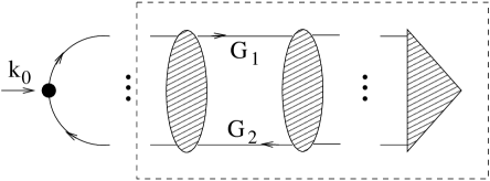
Figure 3: IR-divergent (ladder) diagram. The shaded insertions can represent rungs or self-energy insertions.

The momenta of the propagators $G_{1}$ and $G_{2}$, because of energy–momentum conservation, are $q+k_{0}$ and $q$, respectively. If these propagators are retarded and advanced with the same mass, then for $k_{0}=0$ the poles of the two propagators approach the real axis from above and from below, thus “pinching” it, giving the divergent result $G_{R}(q)G_{A}(q)\sim(\delta(q^{2}-m^{2}))^{2}$ [8, 9]. For finite $k_{0}$ we do not expect divergences, but the $k_{0}\to 0$ limit must be infinite. In Appendix A we indeed find that, at the $k_{0}\to 0$ limit, we have a singular behaviour for the products

$$G_{R}\left(q+\frac{k}{2}\right)G_{A}\left(q-\frac{k}{2}\right)\to i\varrho(q)\frac{d(q)}{2q_{0}k_{0}},\qquad G_{R/A}\left(q+\frac{k}{2}\right)G_{rr}\left(q-\frac{k}{2}\right)\to\frac{d(q)}{2q_{0}k_{0}}G_{rr}(q),$$ (25)

and the inclusion of $G_{R}(q+k/2)$ yields an extra $d(q)/2q_{0}k_{0}$ factor, while the inclusion of additional $G_{A}(q-k/2)$ yields $-d(q)/2q_{0}k_{0}$. Therefore a ladder containing $n$ rungs or self-energy insertions may yield a $k_{0}^{-n}$ IR divergence, corresponding exactly to our expectations.

We can also argue that more particle intermediate states do not give pinch singularities in the massive case. Consider a 3-particle intermediate state with momenta $p,\,q$ and $-p-q$ ($k=0$ case). We expect an IR enhancement if the sum of two momenta is almost zero; let us take $q\approx p+q$, i.e. $p\approx 0$. Then the propagator with momentum $p$ gives $1/m^{2}$, where its mass is $m$, the other two propagators are replaced using Appendix A. One finds, concentrating on this region,

$$\sim d^{4}p\,d^{4}q\,\frac{\varrho(q)}{m^{2}}\,\frac{1}{2p_{0}q_{0}-\omega^{2}_{p+q}+\omega^{2}_{q}}.$$ (26)

This expression is IR-safe, as can be seen for example by integrating over the IR region $|p_{0}|,|{\bf p}|<\varepsilon$. Therefore we cannot have any $1/k_{0}$ enhancement from this insertion. This argumentation can be extended to more internal lines.

There exists another possibility when there is an IR sub-divergence, coming from a self-energy insertion on an internal line. Since, however, internal lines are equilibrium propagators, these pathologies must finally cancel [8].

To resum the ladder diagrams we perform point splitting in a symmetric way:

$$\left\langle{J_{\mu}(x)}\right\rangle=\lim\limits_{y\to x}(i\partial^{x}_{\mu}-i\partial^{y}_{\mu})\frac{1}{2}\left\langle{\Psi(x)\Psi^{\dagger}(y)+\Psi^{\dagger}(y)\Psi(x)}\right\rangle=\lim\limits_{y\to x}(i\partial^{x}_{\mu}-i\partial^{y}_{\mu})i{\cal G}_{rr}^{\Psi}(x,y),$$ (27)

and similarly for $\chi$, where we used R/A formalism to define the propagator [23]. The ${\cal G}$ propagator corresponds to the boxed part in the diagram of Fig. 3. In Fourier space

$$\left\langle{J_{\mu}(k)}\right\rangle={\int\!\frac{d^{4}q}{(2\pi)^{4}}\,}(2q+k)_{\mu}i{\cal G}_{rr}(q+k,q).$$ (28)

Introducing Wigner transformation

$${\cal W}(q,X)=\int d^{4}u\,e^{-iqu}i{\cal G}(X+\frac{u}{2},X-\frac{u}{2}),\qquad{\cal W}(q,k)=i{\cal G}(q+\frac{k}{2},q-\frac{k}{2})$$ (29)

we can rewrite it as

$$\left\langle{J_{\mu}(k)}\right\rangle={\int\!\frac{d^{4}q}{(2\pi)^{4}}\,}2q_{\mu}{\cal W}_{rr}^{\Psi}(q,k).$$ (30)

A ladder diagram is a recursive structure, thus there must be a kernel which relates a ladder containing $N+1$ and $N$ insertions. Keeping only the pinch singular terms we can write $i{\cal G}^{N+1}(p,p^{\prime})=1/{2k_{0}q_{0}}(K*i{\cal G}^{N})(p,p^{\prime})$, where $q=(p+p^{\prime})/2$ and $k=p-p^{\prime}$ (cf. (25)). The sum for all ladders ${\cal G}=\sum_{N}{\cal G}^{N}$ then satisfies $i{\cal G}(p,p^{\prime})=1/{2k_{0}q_{0}}(K*i{\cal G})(p,p^{\prime})$. With the Wigner transformed functions (29), this can be written as ${\cal W}(q,k)=1/{2k_{0}q_{0}}(K*{\cal W})(q,k)$, or, in real space (performing a Fourier transformation with respect to $k$),

$$2iq_{0}\partial_{t}{\cal W}(q,t)=(K*{\cal W})(q,t),$$ (31)

a first order differential equation.

This differential equation is unique up to leading order in the $k$ expansion. Let us assume, namely, that there is another equation

$$2iq_{0}\partial_{t}{\cal W}(q,t)=(K^{\prime}*{\cal W})(q,t)$$ (32)

satisfied by ${\cal W}$. Then inserting the solution of (31) into this equation we find

$$(K-K^{\prime})*{\cal W}=0.$$ (33)

This is an identity that must be fulfilled for $K$ and $K^{\prime}$. This shows that $K=K^{\prime}$ on the space of the solutions of (31).

Using this property we can use differential equations of the form of (31) with different origin in order to resum pinch singularities. And exactly of this form are the Kadanoff–Baym equations [20] in linear response. For the free theory, namely, the propagators satisfy, because of the Schwinger–Dyson equations,

$$(\partial_{x}^{2}-\partial_{y}^{2}){\cal G}(x,y)=0\quad\Rightarrow\quad 2iq_{0}\partial_{t}{\cal W}(q,t)=0.$$ (34)

In the case of interactions the right-hand side depends on ${\cal G}$ (or ${\cal W}$), but in the linear response theory it is linearized and has the form $K*{\cal W}$ with some kernel. We therefore recover (32). The uniqueness of this equation then implies that the Kadanoff–Baym equations represent an adequate tool to resum the pinch singularities of ladder diagrams in linear response theory.

So finally both the coordinate space method [7] and the momentum space method outlined above support the statement that the resummation of $1/k_{0}^{n}$ IR singularities of the perturbation theory yields quantum Boltzmann equations (Kadanoff–Baym equations). Therefore $\Gamma$ appearing in (23) must be calculated using Boltzmann equations.

In our model to lowest order we have to take into account the decay processes, which have a matrix element $h$. Therefore the Boltzmann equations are

$$2q\partial_{X}N^{\Psi}(q,X)=h^{2}{\int\!\frac{d^{4}\ell}{(2\pi)^{4}}\,}\varrho^{\chi}(\ell)\varrho^{\Phi}(q-\ell)\left[(N^{\Psi}+1)N^{\chi}N^{\Phi}-N^{\Psi}(1+N^{\chi})(1+N^{\Phi})\right],$$ (35)

and similar equations for $\chi$ and $\Phi$. In the integrand we denoted $N^{\Psi}(q,X)\to N^{\Psi}$, $N^{\chi}(\ell,X)\to N^{\chi}$ and $N^{\Phi}(q-\ell,X)\to N^{\Phi}$. The possible values of $q_{0}$ are $q_{0}=\pm\omega_{\bf q}$ (the dispersion relation).

We solve the equations in the relaxation time approximation. We rewrite (30) using our condition that there is no net charge in equilibrium

$$Q^{\Psi}(t)={\int\!\frac{d^{4}q}{(2\pi)^{4}}\,}2q_{0}\varrho^{\Psi}(q)\delta N(q,t),$$ (36)

where $\delta N$ is the deviation from equilibrium. For $\delta N$ the linearized equation reads

$$2q\partial_{X}\delta N^{\Psi}=-h^{2}{\int\!\frac{d^{4}\ell}{(2\pi)^{4}}\,}\varrho^{\chi}\varrho^{\Phi}\left[\delta N^{\Psi}\!\left(1+N^{\chi}+N^{\Phi}\right)+\delta N^{\chi}\!\left(N^{\Psi}-N^{\Phi}\right)+\delta N^{\Phi}\!\left(N^{\Psi}-N^{\chi}\right)\right].$$ (37)

We multiply this equation by $\varrho^{\Psi}(q)$ and integrate over $q$. We can realize that, because $\Phi$ is a real field,

$${\cal G}_{rr}^{\Phi}(x,y)={\cal G}_{rr}^{\Phi}(y,x)\quad\Rightarrow\quad{\cal G}_{rr}^{\Phi}(p,p^{\prime})={\cal G}_{rr}^{\Phi}(-p^{\prime},-p)\quad\Rightarrow\quad\delta{\cal W}^{\Phi}(q,k)=\delta{\cal W}^{\Phi}(-q,k).$$ (38)

Since $\delta{\cal W}=\varrho^{\Phi}\delta N$ [17], this symmetry renders the last term of (37) zero after integration. We introduce

$$\Gamma^{\Psi}(q)=\frac{h^{2}}{2q_{0}}{\int\!\frac{d^{4}\ell}{(2\pi)^{4}}\,}\varrho^{\chi}(\ell)\varrho^{\Phi}(q-\ell)(1+N(\ell_{0})+N(q_{0}-\ell_{0}))=\frac{-2\,\textrm{Im}\,\Pi_{R}^{\Psi}(q)}{2q_{0}},$$

$$\Gamma^{\chi}(q)=\frac{h^{2}}{2q_{0}}{\int\!\frac{d^{4}\ell}{(2\pi)^{4}}\,}\varrho^{\Psi}(\ell)\varrho^{\Phi}(q-\ell)(1+N(\ell_{0})+N(q_{0}-\ell_{0}))=\frac{-2\,\textrm{Im}\,\Pi_{R}^{\chi}(q)}{2q_{0}},$$ (39)

where $N(x)=(e^{\beta x}-1)^{-1}$ is the Bose–Einstein distribution, and write

$$\partial_{t}Q^{\Psi}(t)={\int\!\frac{d^{4}q}{(2\pi)^{4}}\,}\left[-2q_{0}\delta N^{\Psi}(q,t)\varrho^{\Psi}\Gamma^{\Psi}(q)+2q_{0}\delta N^{\chi}(q,t)\varrho^{\chi}\Gamma^{\chi}(q)\right].$$ (40)

The relaxation time approximation assumes that $\Gamma$ is only weakly momentum-dependent, so we can factorize the integral, and we finally obtain

$$\partial_{t}Q^{\Psi}(t)=-\Gamma^{\Psi}Q^{\Psi}(t)+\Gamma^{\chi}Q^{\chi}(t),$$

$$\partial_{t}Q^{\chi}(t)=-\Gamma^{\chi}Q^{\chi}(t)+\Gamma^{\Psi}Q^{\Psi}(t).$$ (41)

This approximation satisfies the requirement that $Q^{\Psi}+Q^{\chi}=\mathrm{const.}$, which is zero (the equilibrium value). Then the solution of the above equations is

$$Q^{\Psi}(t)=Q^{\Psi}(0)e^{-(\Gamma^{\Psi}+\Gamma^{\chi})t},\qquad Q^{\chi}(t)=-Q^{\Psi}(0)e^{-(\Gamma^{\Psi}+\Gamma^{\chi})t}.$$ (42)

For $m_{\Psi}\gg m_{\chi},m_{\Phi}$ we find

$$\Gamma^{\Psi}=\frac{h^{2}}{16\pi m_{\Psi}}\left(1+2N(\frac{m_{\Psi}}{2})\right),\qquad\Gamma^{\chi}=\frac{h^{2}}{16\pi m_{\chi}}\beta MN(M)(1+N(M)),$$ (43)

where $M=m_{\Psi}^{2}/2m_{\chi}$.

4 Contributions coming from analytic defects

The other important ingredient of the long-time evolution is the power law tail coming from analytic defects of the spectral function. These, in general (cf. Section 2), yield the time dependence $A\cos(\Omega t+\phi)/t^{\alpha+1}$. The value of $\Omega$ and $\alpha$ depends on the theory, while the amplitude $A$ and the phase $\phi$ come from the initial conditions. In this section we try to compute $\Omega$ and $\alpha$ for some special cases.

4.1 Two-particle cut

Let us first consider a diagram where there is a two-particle intermediate state, as is illustrated in Fig. 4a.

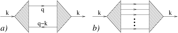
Figure 4: Two- and multiparticle intermediate state

We represent it as two momentum-dependent vertices denoted by $\Gamma_{1}(q,k)$ and $\Gamma_{2}(q,k)$, their product being denoted by $\Gamma=\Gamma_{1}\Gamma_{2}$. The intermediate particles have masses $m_{1}$ and $m_{2}$, and we treat it as a cut diagram (with Keldysh indices $21$ minus $12$). Its contribution then is

$$C_{2}(k) ={\int\!\frac{d^{4}q}{(2\pi)^{4}}\,}\Gamma(q,k)\left[G_{1}^{21}(q)G_{2}^{21}(k-q)-G_{1}^{12}(q)G_{2}^{12}(k-q)\right]$$ (44)

$$=4\pi^{2}{\int\!\frac{d^{4}q}{(2\pi)^{4}}\,}\frac{\Gamma(q,k)}{4\omega_{1}\omega_{2}}[(1+N(q_{0}))(1+N(k_{0}-q_{0}))-N(q_{0})N(k_{0}-q_{0})]$$

$$\hskip 56.9055pt\times(\delta(q_{0}-\omega_{1})-\delta(q_{0}+\omega_{1}))(\delta(k_{0}-q_{0}-\omega_{2})-\delta(k_{0}-q_{0}+\omega_{2})).$$

The analytic defects of this function are thresholds, where the phase-space, restricted by the constraints of the integration, vanishes. There are 4 such points in this case: $k_{0}=\pm m_{1}\pm m_{2}$. We restrict ourselves for positive $k_{0}$ and denote $k^{(1)}_{0}=m_{1}+m_{2}$ and $k^{(2)}_{0}=m_{1}-m_{2}$ (assuming $m_{1}\geq m_{2}$). At $k^{(1)}$ a cut starts, at $k^{(2)}$ it stops, so for the threshold behaviour we choose $k_{0}=k^{(1)}_{0}+y$ or $k_{0}=k^{(2)}_{0}-y$. Since for $y\to 0$ the phase space vanishes (${\bf q}\to 0$), we can expand everything to second order with respect to $|{\bf q}|$.

In the $k^{(1)}$ case the relevant combination of the delta functions of (44) is

$$\delta(q_{0}-\omega_{1})\delta(k_{0}-q_{0}-\omega_{2})\quad\Rightarrow\quad k_{0}=\omega_{1}+\omega_{2}.$$ (45)

Expanding $\omega_{1}+\omega_{2}$ around $k^{(1)}_{0}=m_{1}+m_{2}$ to second order yields

$$y=\left(\frac{1}{2m_{1}}+\frac{1}{2m_{2}}\right){\bf q}^{2},$$ (46)

so that $|{\bf q}|$ vanishes as $y^{1/2}$. Assuming that $\Gamma$ does not vanish in this limit (as the best case), and we substitute $\omega_{1,2}\to m_{1,2},\,k_{0}=m_{1}+m_{2}$ and ${\bf q}=0$ where it is possible, we find

$$C\sim(1+N(m_{1})+N(m_{2})){\int\!\frac{d^{3}{\bf q}}{(2\pi)^{3}}\,}\delta\left(y-\left(\frac{1}{2m_{1}}+\frac{1}{2m_{2}}\right){\bf q}^{2}\right)\sim y^{1/2},$$ (47)

which can be seen after performing the integral. This is the same as the zero-temperature result [21], only the amplitude is modified by $(1+N(m_{1})+N(m_{2}))$.

The $k^{(2)}$ case goes along the same lines. We choose the combination

$$\delta(q_{0}-\omega_{1})\delta(k_{0}-q_{0}+\omega_{2})\quad\Rightarrow\quad k_{0}=\omega_{1}-\omega_{2}\quad\Rightarrow\quad y=\left(\frac{1}{2m_{2}}-\frac{1}{2m_{1}}\right){\bf q}^{2},$$ (48)

and therefore

$$C\sim(N(m_{1})-N(m_{2}))y^{1/2}.$$ (49)

This is a finite temperature effect, the threshold of the Landau cut [19].

For our concrete example described by the Lagrangian (1), only equal-mass two-particle intermediate states are allowed. In that case the first threshold is just a zero temperature one, starting at $2m_{i}$ where $m_{i}\in\{m,M,m_{S}\}$. The second case, however, is not present, since the delta constraints then give $\delta(k_{0})$. So there the important cut contribution has $\Omega=2m_{i}$ and $\alpha=1/2$. That is we obtain an oscillating contribution which has presumably negligible effect on real physical processes.

4.2 Four-particle intermediate state

Four-particle intermediate states may contain cuts, and this will be analyzed in the next subsection. Here we concentrate on other possible analytic defects.

On the same footing as before we can write up the contribution coming from the four-particle intermediate state

$$C_{4}(k)={\int\!\frac{d^{4}q_{1}}{(2\pi)^{4}}\,}..\frac{d^{4}q_{4}}{(2\pi)^{4}}\,\delta(k-{\textstyle\sum}q)\Gamma(k,\{q\})\left[(1+N_{1})..(1+N_{4})-N_{1}..N_{4}\right]\varrho_{1}(q_{1})..\varrho_{4}(q_{4}),$$ (50)

where $N_{i}=N(q_{0i})$. We change $q\to-q$ in the first term and write $C_{4}(k)=C_{4}^{+}(k)-C_{4}^{-}(k)$ where

$$C_{4}^{\pm}(k)={\int\!\frac{d^{4}q_{1}}{(2\pi)^{4}}\,}..\frac{d^{4}q_{4}}{(2\pi)^{4}}\,\delta(k\pm{\textstyle\sum}q)\Gamma(k,\{\mp q\})N_{1}..N_{4}\,\varrho_{1}..\varrho_{4}.$$ (51)

In fact, this is a general form; we can write also for the two-particle contribution (44) $C_{2}(k)=C_{2}^{+}(k)-C_{2}^{-}(k)$, where

$$C_{2}^{\pm}(k)={\int\!\frac{d^{4}q_{1}}{(2\pi)^{4}}\,}\frac{d^{4}q_{2}}{(2\pi)^{4}}\,\delta(k\pm{\textstyle\sum}q)\Gamma(k,\{\mp q\})N_{1}N_{2}\,\varrho_{1}\varrho_{2}.$$ (52)

We now make a simplification, and assume that for some reason $\Gamma$ is factorized as $\Gamma(k,\{q\})=\Gamma^{(1,2)}(k,q_{1},q_{2})\Gamma^{(3,4)}(k,q_{3},q_{4})$. This means a loss in generality; but we hope that the main consequences still remain true. We introduce an auxiliary variable $Q$ and write

$$C_{4}^{+}(k)={\int\!\frac{d^{4}Q}{(2\pi)^{4}}\,} {\int\!\frac{d^{4}q_{1}}{(2\pi)^{4}}\,}\!\frac{d^{4}q_{2}}{(2\pi)^{4}}\,\delta(Q+q_{1}+q_{2})\Gamma^{(1,2)}(k,-q_{1},-q_{2})N_{1}N_{2}\varrho_{1}(q_{1})\varrho_{2}(q_{2})$$

$$\times {\int\!\frac{d^{4}q_{3}}{(2\pi)^{4}}\,}\!\frac{d^{4}q_{4}}{(2\pi)^{4}}\,\delta(k-Q+q_{3}+q_{4})\Gamma^{(3,4)}(k,-q_{3},-q_{4})N_{3}N_{4}\varrho_{3}(q_{3})\varrho_{4}(q_{4}).$$ (53)

On the right-hand side we recover the convolution of two $C_{2}^{+}$ contributions; in real time they are simply multiplied. The complete four-particle contribution can be written as

$$C_{4}(t)=C_{2}^{+}(t){C^{\prime}_{2}}^{+}(t)-C_{2}^{-}(t){C^{\prime}_{2}}^{-}(t).$$ (54)

At zero temperature $N(q_{0})\to-\Theta(-q_{0})$, thus $C_{2}^{+}$ contains only the positive energy cuts and $C_{2}^{+}{C^{\prime}}_{2}^{+}$ oscillates with frequency $\Omega+\Omega^{\prime}$. At finite temperature, however, the negative energy cut appears as well, and, for the same threshold values, we have

$$\frac{A_{-}e^{i\Omega t}+A_{+}e^{-i\Omega t}}{t^{3/2}}\frac{A^{\prime}_{-}e^{i\Omega t}+A^{\prime}_{+}e^{-i\Omega t}}{t^{3/2}}=\frac{A_{-}A^{\prime}_{+}+A_{+}A^{\prime}_{-}}{t^{3}}+\mathrm{oscillating}.$$ (55)

Diagrammatically it comes from the diagram where two lines are incoming, two are outgoing, or vice versa. Kinematically, with the external line, it is a $2\to 3$ or $3\to 2$ process. Also from here we see that this contribution must be absent at zero temperature. We can assess the temperature dependence by the typical factor for 2 incoming and 2 outgoing internal lines,

$$(1+N(m_{1}))(1+N(m_{2}))N(m_{3})N(m_{4}).$$ (56)

For low temperatures the contribution is therefore Boltzmann-suppressed.

We can also have cancellations at finite temperature, if the $+$ and $-$ parts in (54) cancel each other. $C^{+}$ and $C^{-}$ are related as (writing out explicitly the dependence on the $\Gamma$ vertex function)

$$C^{+}(\Gamma,-k)=C^{-}(\tilde{\Gamma},k),\quad\mathrm{where}\quad\tilde{\Gamma}(k,\{q\})=\Gamma(-k,\{-q\}).$$ (57)

Cancellation occurs, if $\tilde{\Gamma}=\pm\Gamma$ for small $k$. For generic $F$ at finite temperature we do not expect such a symmetry, therefore a net effect will remain.

How can this phenomenon show up in a diagram? If we calculate $Q(k_{0})$ for small $k_{0}$, we encounter ladder diagrams, as is shown in Fig. 3. The ending of the ladder (the triangle at the right-hand side) contributes to the numerator (the constant $C$ in eq. (23)). Here can sit the four-particle intermediate state of this section, see for example Fig. 5.

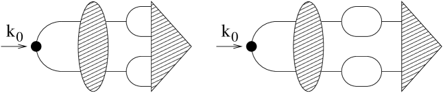
Figure 5: The realization of a four-particle internal state. The shaded oval denotes ladder resummation.

The $k_{0}\approx 0$ behaviour of the charge is therefore

$$Q(k_{0}\to 0)\sim\frac{\zeta_{2}+\#C_{4}(k_{0})h^{4}\zeta_{2}+\#C_{4}(k_{0})h^{2}\zeta_{4}}{k_{0}+i\Gamma}.$$ (58)

The pole and the $k_{0}=0$ defects are therefore separated and do not affect the behaviour of each other. When computing the numerical coefficient of the $k_{0}=0$ defect we substitute $k_{0}=0$ in the numerator, which means an enhancement factor of $1/\Gamma$.

Four-particle initial conditions can also come from the quadratic response (as a product of two two-particle operators). Having the same effect, it is natural to assume that their contribution is also in the same order of magnitude, i.e. $\zeta_{4}\sim\zeta_{2}^{2}$. Since $\zeta\ll 1$ (linear response regime) we find suppression in this term. To have only one small parameter in the system we will assume that $\zeta_{2}\sim h^{2}$.

Summarizing, the $1/t^{3}$ contribution of the four-particle intermediate state is suppressed by several effects compared to the Boltzmann pole. It has a perturbative suppression of $h^{2}$; it is a finite-temperature effect, so that it is Boltzmann-suppressed at small temperatures; it has two contributions with opposite sign; and finally it is a multiloop effect, which probably means also a numerical suppression.

4.3 Multiparticle cuts and other defects

The determination of the threshold behaviour described in the case of two-particle intermediate states can be generalized to multiparticle intermediate states (cf. Fig. 4b). We expect thresholds when the external $k_{0}$ plus the $N$ internal particles represent a decay process ($1\to N$ or $N\to 1$), since scattering processes do not have cuts. There always exists a possibility, when all of the internal particles are outgoing, so that $k^{(1)}_{0}=\sum_{i}m_{i}$ is the threshold value; this is also the zero-temperature case. At finite temperature an additional threshold is possible (for positive $k_{0}$), when one particle is outgoing, the rest are incoming. Then we obtain a threshold at $k_{0}^{(2)}=m_{1}-\sum_{i=2}^{N}m_{i}$, if it is positive.

Near the threshold, in the massive case, we can perform the same expansion as in (46), and also there is a momentum-conserving delta function $\delta(\sum{\bf q}_{i})$. Therefore what remains is

$$\int d^{3}{\bf q}_{1}\dots d^{3}{\bf q}_{N}\delta\left(y-\sum_{i}\frac{{\bf q}_{i}^{2}}{2m_{i}}\right)\delta\left(\sum_{i}q_{i}\right)\sim y^{\frac{3N}{2}}y^{-1}y^{-\frac{3}{2}}\sim y^{\frac{3(N-1)}{2}-1}.$$ (59)

The possible values for $\Omega$ thus are $\sum_{i}m_{i}$ and $m_{1}-\sum_{i>1}m_{i}$ (if it is positive), in both cases $\alpha=\frac{3(N-1)}{2}-1$ (which is also the zero-temperature result).

Similarly to the two times two-particle cut case, multiparticle cuts can also be multiplied in real space to generate new defects. This means, however, a faster decay than $1/t^{3}$.

5 Conclusions

In this paper we tried to describe the time evolution of the charge operator $Q$ in a complex scalar system, starting from an initial state not too far from thermal equilibrium. The initial state was prepared using an external action that modifies the time evolution for a given period. We applied linear response theory in the external action to describe time evolution. As a computing method we used real time perturbation theory.

The long-time behaviour of $Q$ is determined by the $QF$ spectral function in the linear response theory, where $F$ is an arbitrary operator ($[Q,F]\neq 0$). If $Q$ were conserved, there would be $\varrho^{(QF)}(k_{0})\sim\delta(k_{0})$. For the non-conserving case two types of contributions can be identified (cf. [1, 5, 6]). One is coming from the broadening of the $\delta(k_{0})$ pole of the conserved $Q$-case, yielding exponential damping for long times. In perturbation theory it manifests itself as pinch singularities in the ladder diagrams, giving $1/k_{0}^{n}$ type of IR divergences at any order in the coupling. Resummation of these singularities results in linearized Kadanoff–Baym equations. Working in real space, $1/k_{0}^{n}$ singularities correspond to the secular terms $t^{n-1}$, and their resummation also leads to quantum Boltzmann equations [7].

Analytic defects in $\varrho^{(QF)}(k_{0})$ also contribute to long-time physics: it gives an $e^{-i\Omega t}/t^{\alpha+1}$ oscillating power-law decay, where $\Omega$ is the position of the defect, $\alpha$ is the index of $\varrho$ near to the defect. For multiparticle cuts we have $\Omega=\sum_{i}m_{i}$ or $m_{i}-\sum_{i>1}m_{i}$ (if it is positive: a multiparticle Landau damping), and index $\alpha=3(N-1)/2-1$, where $N$ is the number of intermediate particles and $m_{i}$ are their masses. These contributions are oscillating with the particle mass, so that they can hardly influence physics on IR scales. At finite temperature, however, these cuts can be combined, and from their superposition the oscillating behaviour can drop out. The lowest order diagram giving this result contains 4 intermediate particles and yields $1/t^{3}$ type of decay.

So finally, starting from a generic initial state characterized by $F$, we expect that the time evolution of the charge for large times follows

$$Q(t)=Q_{1}e^{-\Gamma t}+\frac{Q_{2}}{t^{3}}+\mathrm{oscillating}.$$ (60)

The relative weights of the Boltzmann pole and the cut contributions contain free parameters, depending on the initial state, and they contain perturbative factors. The pole is present already at the free level, we thus expect $Q_{1}={\cal O}(1)\,+$ perturbative corrections. The amplitude of $Q_{2}$ is reduced by several effects; for example it is suppressed by $h^{2}$ and by the Boltzmann factor for small temperatures. Thus, for a generic situation we expect that exponential damping dominates the time evolution for intermediate times and only after a long time will the power law take over (for a numerical simulation example see, [22]). Still, because of its slow decay, it can be relevant in the explanation of small deviations from equilibrium (such as baryogenesis). This should be examined in the future.

Another task for the future is to include non-linear effects and see how the full Boltzmann equation gets modified due to the presence of cut contributions.

Appendix A Appendix: pinch singularities

The pole structure of the retarded and advanced propagators is represented by

$$D_{R/A}(q)=\frac{1}{(q_{0}\pm i\varepsilon)^{2}-\omega^{2}}=\frac{1}{2\omega}\left[\frac{1}{q_{0}-\omega\pm i\varepsilon}-\frac{1}{q_{0}+\omega\pm i\varepsilon}\right]$$ (61)

where $\omega({\bf q})$ is the dispersion relation. They have poles at $\pm\omega-i\varepsilon$ for the retarded Green’s function and $\pm\omega+i\varepsilon$ for the advanced one. Their product thus has poles at $\pm\omega\pm i\varepsilon$, which pinch the real axis for $\varepsilon\to 0$, resulting in double poles which cannot be regularized. We do not expect such problems for products like $D_{R}D_{R}$ or $D_{A}D_{A}$.

In our case the momenta of the retarded and advanced propagators are offset by $k$. For finite $k$ we do not expect singularities, but the $k\to 0$ limit must be divergent.

First we examine the $D_{R}(q+k)D_{A}(q)$ product for small $k=(k_{0},0)$. We will use the identity

$$\frac{1}{x+i\varepsilon}=\mathop{\cal P}\left(\frac{1}{x}\right)-i\pi\delta(x)$$ (62)

where ${\cal P}$ means principal value, so that

$$D_{R/A}(q)=\frac{1}{2\omega}\left[\mathop{\cal P}\left(\frac{1}{q_{0}-\omega}\right)\mp i\pi\delta(q_{0}-\omega)-\{\omega\to-\omega\}\right].$$ (63)

For the product we obtain

$$D_{R}(q+\frac{k}{2})D_{A}(q-\frac{k}{2})=\frac{1}{4\omega^{2}}\biggl{[}\! i\pi\mathop{\cal P}\left(\frac{1}{k_{0}}\right)\left(\delta(q_{0}-\frac{k_{0}}{2}-\omega)+\delta(q_{0}+\frac{k_{0}}{2}-\omega)\right)$$ (64)

$$+\pi^{2}\delta(k_{0})\delta(q_{0}-\omega)+\,\{\omega\to-\omega\}\biggr{]}+\textrm{non-singular},$$

the non-singular terms having finite limit at $k\to 0$. Rewriting this expression we obtain

$$D_{R}(q+\frac{k}{2})D_{A}(q-\frac{k}{2})=i\mathop{\cal P}\left(\frac{1}{2q_{0}k_{0}}\right)\varrho(q)+o\left(\frac{1}{k_{0}}\right),$$ (65)

where $\varrho$ is the free spectral function; $o(1/x)$ means that $\lim_{x\to 0}(x\,o(1/x))=0$, which is trivial for non-singular terms, and true for the delta term since $x\delta(x)=0$.

In a real model we can write for the propagator $G(q)=d(q)D(q)$, where $d$ is the Klein–Gordon divisor [8].

We can obtain (65) in a different way, using $i(G_{R}-G_{A})=\varrho$ and that $G_{R}G_{R}$ is non-singular. We write

$$G_{R}(q+\frac{k}{2})G_{A}(q-\frac{k}{2})=G_{R}(q+\frac{k}{2})\,i\varrho(q-\frac{k}{2})-G_{R}(q+k)G_{R}(q).$$ (66)

The second term is finite for $k\to 0$, while in the first term at $k=0$ we put a propagator on mass shell, which is clearly divergent. The numerator of $G_{R}(q+k/2)$ for small $k$ reads

$$q_{0}^{2}+q_{0}k_{0}+\frac{k_{0}^{2}}{4}-\omega_{{\bf q}+{\bf k}/2}^{2}\to 2q_{0}k_{0}+\omega_{{\bf q}-{\bf k}/2}^{2}-\omega_{{\bf q}+{\bf k}/2}^{2}\to 2q_{0}k_{0}-2{\bf k}\cdot\partial\omega,$$ (67)

where we have power-expanded $\omega_{{\bf q}\pm{\bf k}/2}$. Therefore

$$G_{R}(q+\frac{k}{2})G_{A}(q-\frac{k}{2})=\frac{d(q)}{2q_{0}k_{0}-2{\bf k}\cdot\partial\omega}\,i\varrho(q)+\dots,$$ (68)

where $d(q)$ is the Klein–Gordon divisor. It is also clear that any other $G_{R}$ factor yields the same $d(q)/(2q_{0}k_{0}-2{\bf k}\cdot\partial\omega)$ contribution. Additional $G_{A}$ factors yield $-d(q)/(2q_{0}k_{0}-2{\bf k}\cdot\partial\omega)$ contribution, as can be seen by using the above formulae for $G_{R}=-i\varrho+G_{A}$.

In the paper we use $k=(k_{0},0)$ momentum, but all the formulae can easily be generalized to finite ${\bf k}$ simply by $2q_{0}k_{0}\to 2q_{0}k_{0}-2{\bf k}\cdot\partial\omega$.

Pinch singularities occur in other products as well. In the R/A formalism [23] the propagators are $G_{R},\,G_{A}$ and $G_{rr}=(G_{12}+G_{21})/2$. Since $G_{rr}\sim\varrho$ also puts the propagation on the mass shell, we find

$$G_{R/A}(q+\frac{k}{2})G_{rr}(q-\frac{k}{2})=\frac{d(q)}{2q_{0}k_{0}}G_{rr}(q).$$ (69)

On the other hand $G_{rr}(q+k)\cdot G_{rr}(q)\sim\delta(k_{0})$, therefore it yields an $o(1/k_{0})$ contribution. So in the two-particle intermediate states the possible pinch enhancements are coming from $G_{R}G_{A}$ and $G_{rr}G_{R/A}$ only.

References

- [1] I. Joichi, Sh. Matsumoto and M. Yoshimura, Phys. Rev. D58 (1998) 043507; Sh. Matsumoto and M. Yoshimura, Phys. Rev. D59 (1999) 123511; Sh. Matsumoto and M. Yoshimura, Phys. Rev. D61 (2000) 123508; Sh. Matsumoto and M. Yoshimura, Phys. Rev. D61 (2000) 123509
- [2] M. Srednicki, Phys. Rev. D62 (2000) 023505
- [3] E. Braaten and Y. Jia, Phys. Rev. D63 (2001) 096009
- [4] P. Bucci and M. Pietroni, Phys. Rev. D63 (2001) 045026; P. Bucci and M. Pietroni, hep-ph/0111375
- [5] D. Boyanovsky, I. D. Lawrie and D. S. Lee, Phys. Rev. D54 (1996) 4013; D. Boyanovsky, M. D’Attanasio, H. J. de Vega and R. Holman, Phys. Rev. D54) (1996) 1748
- [6] A. Jakovác, A. Patkós, P. Petreczky and Z. Szép, Phys. Rev. D61 (2000) 025006
- [7] D. Boyanovsky, H. J. de Vega and S.-Y. Wang, Phys. Rev. D61 (2000) 065006
- [8] N. P. Landsmann and Ch. G. van Weert, Phys. Rep. 145 (1987) 141
- [9] T. Altherr and D. Seibert, Phys. Lett. B333 (1994) 149
- [10] M. E. Carrington, Hou Defu and M. H. Thoma, Eur. Phys. J. C7 (1999) 347
- [11] C. Greiner and S. Leupold, Eur. Phys J. C8 (1999) 517
- [12] G. D. Mahan, Many particle physics (New York, Plenum, 1990)
- [13] J. S. Langer, Phys. Rev. 120 (1960) 714
- [14] M. E. Carrington, H. Defu and R. Kobes, hep-ph/0106292
- [15] S. Jeon and L. G. Yaffe, Phys. Rev. D53 (1996) 5799
- [16] P. Arnold, G. D. Moore and L. G. Yaffe, hep-ph/0109064; P. Arnold, G. D. Moore and L. G. Yaffe, hep-ph/0111107
- [17] W. Buchmüller and S. Fredenhagen, Phys. Lett. B483 (2000) 217
- [18] E. Mottola and S. Raby, Phys. Rev. D42 (1990) 4202; D. N. Zubarev Teor. Mat. Fiz. 3 (1970) 276
- [19] M. Le Bellac, Thermal field theory (University Press, Cambridge, 1996)
- [20] L. P. Kadanoff, G. A. Baym, Quantum statistical mechanics : Green’s function methods in equilibrium and non-equilibrium problems (Menlo Park, Benjamin, 1962); S. Mrowczynski and U. Heinz, Ann. Phys. (N.Y.) 229 (1994) 1
- [21] R. J. Eden, P. V. Landshoff, D. I. Olive and J. Ch. Polkinghorne, The analytic S-matrix, (University Press, Cambridge, 1966)
- [22] Sz. Borsányi and Zs. Szép, Phys. Lett. B508 (2001) 109
- [23] E. Wang and U. Heinz, Phys. Lett. B471 (1999) 208; K.-C. Chou, Z.-B. Su, B.-L. Hao and L. Yu, Phys. Rep. 118 (1985) 1