Radiative return at NLO and the measurement of the
hadronic cross-section in electron–positron annihilation

Abstract

Electron–positron annihilation into hadrons plus an energetic photon from initial state radiation allows the hadronic cross-section to be measured over a wide range of energies. The full next-to-leading order QED corrections for the cross-section for $e^{+}e^{-}$ annihilation into a real tagged photon and a virtual photon converting into hadrons are calculated where the tagged photon is radiated off the initial electron or positron. This includes virtual and soft photon corrections to the process $e^{+}e^{-}\rightarrow\gamma+\gamma^{*}$ and the emission of two real hard photons: $e^{+}e^{-}\rightarrow\gamma+\gamma+\gamma^{*}$. A Monte Carlo generator has been constructed, which incorporates these corrections and simulates the production of two charged pions or muons plus one or two photons. Predictions are presented for centre-of-mass energies between $1$ and $10$ GeV, corresponding to the energies of DA$\Phi$NE, CLEO-C and $B$-meson factories.

1 Introduction

Electroweak precision measurements have become one of the central issues in particle physics nowadays. The recent measurement of the muon anomalous magnetic moment $a_{\mu}\equiv(g-2)_{\mu}/2$ at BNL Brown:2001mg led to a new world average, differing by $2.6$ standard deviations from its theoretical Standard Model evaluation Hughes:1999fp . This disagreement, which has been taken as an indication of new physics, has triggered a raving and somehow controversial deluge of non-Standard Model explanations. A new measurement with an accuracy three times better is under way; this will challenge even more the theoretical predictions.

One of the main ingredients in the theoretical prediction for the muon anomalous magnetic moment is the hadronic vacuum polarization contribution hadronicmuon which is moreover responsible for the bulk of the theoretical error. It is in turn related via dispersion relations to the cross-section for electron–positron annihilation into hadrons, $\sigma_{had}=\sigma(e^{+}e^{-}\rightarrow hadrons)$. This quantity plays an important role also in the evolution of the electromagnetic coupling $\alpha_{QED}$ from the low energy Thompson limit to high energies hadronicmuon ; runningQED . This indeed means that the interpretation of improved measurements at high energy colliders such as LEP, the LHC, or the Tevatron depends significantly on the precise knowledge of $\sigma_{had}$.

The evaluation of the hadronic vacuum polarization contribution to the muon anomalous magnetic moment, and even more so to the running of $\alpha_{QED}$, requires the measurement of $\sigma_{had}$ over a wide range of energies. Of particular importance for the QED coupling at $M_{Z}$ is the low energy region around $2$ GeV, where $\sigma_{had}$ is at present poorly determined experimentally and only marginally consistent with the predictions based on pQCD. New efforts are therefore mandatory in this direction, which could help to either remove or sharpen the discrepancy between theoretical prediction and experimental results for $(g-2)_{\mu}$ and provide the basis for future more precise high energy experiments.

The feasibility of using tagged photon events at high luminosity electron–positron storage rings, such as the $\phi$-factory DA$\Phi$NE or $B$-factories, to measure $\sigma_{had}$ over a wide range of energies has been proposed and studied in detail in Binner:1999bt ; Melnikov:2000gs ; Czyz:2000wh (see also Spagnolo:1999mt ; Khoze:2001fs ). In this case, the machine is operating at a fixed centre-of-mass (cms) energy. Initial state radiation (ISR) is used to reduce the effective energy and thus the invariant mass of the hadronic system. The measurement of the tagged photon energy helps to constrain the kinematics, which is of particular importance for multimeson final states. In contrast to the conventional energy scan Akhmetshin:1999uj , the systematics of the measurement (e.g. normalization, beam energy) have to be taken into account only once, and not for each individual energy point independently.

Radiation of photons from the hadronic system (final state radiation, FSR) should be considered as background and can be suppressed by choosing suitable kinematical cuts, or controlled by the simulation, once a suitable model for this amplitude has been adopted. From studies with the generator EVA Binner:1999bt one finds that selecting events with the tagged photons close to the beam axis and well separated from the hadrons indeed reduces FSR to a reasonable limit. Furthermore, the suppression of FSR overcomes the problem of its model dependence, which should be taken into account in a completely inclusive measurement Hoefer:2001mx .

Preliminary experimental results using this method have been presented recently by the KLOE collaboration at DA$\Phi$NE Aloisio:2001xq ; Denig:2001ra ; Adinolfi:2000fv . Large event rates were also observed by the BaBar collaboration babar .

In this paper we consider the full next-to-leading order (NLO) QED corrections to ISR in the annihilation process $e^{+}e^{-}\rightarrow\gamma+hadrons$ where the photon is observed under a non-vanishing angle relative to the beam direction. The virtual and soft photon corrections Rodrigo:2001jr and the contribution of the emission of a second real hard photon are combined to obtain accurate predictions for the exclusive channel $e^{+}e^{-}\rightarrow\pi^{+}\pi^{-}\gamma$ at cms energies of $1$ to $10$ GeV, corresponding to the energies of DA$\Phi$NE, CLEO-C and $B$-meson factories. An improved Monte Carlo generator, denoted PHOKHARA, includes these terms and will be presented in this work. The comparison with the EVA Binner:1999bt Monte Carlo, which simulates the same process at leading order (LO) and includes additional collinear radiation through structure function (SF) techniques, is described. Predictions are presented also for the muon pair production channel $e^{+}e^{-}\rightarrow\mu^{+}\mu^{-}\gamma$, which is also simulated with the new generator.

2 Virtual and soft photon corrections to ISR

Figure 1: One-loop corrections to initial state radiation in $e^{+}e^{-}\rightarrow\gamma+hadrons$.

At NLO, the $e^{+}e^{-}$ annihilation process

$$e^{+}(p_{1})+e^{-}(p_{2})\rightarrow \gamma^{*}(Q)+\gamma(k_{1})~{},$$ (1)

where the virtual photon converts into a hadronic final state, $\gamma^{*}(Q)\rightarrow hadrons$, and the real one is emitted from the initial state, receives contributions from one-loop corrections (see Fig. 1) and from the emission of a second real photon (see Fig. 2).

After renormalization the one-loop matrix elements still contain infrared divergences. These are cancelled by adding the contribution where a second photon has been emitted from the initial state. This rate is integrated analytically in phase space up to an energy cutoff $E_{\gamma}<w\sqrt{s}$ far below $\sqrt{s}$. The sum Rodrigo:2001jr is finite; however, it depends on this soft photon cutoff. The contribution from the emission of a second photon with energy $E_{\gamma}>w\sqrt{s}$ completes the calculation and cancels this dependence.

In order to facilitate the extension of the Monte Carlo simulation to different hadronic exclusive channels the differential rate is cast into the product of a leptonic and a hadronic tensor and the corresponding factorized phase space:

$$d\sigma=\frac{1}{2s}L_{\mu\nu}H^{\mu\nu}d\Phi_{2}(p_{1},p_{2};Q,k_{1})d\Phi_{n}(Q;q_{1},\cdot,q_{n})\frac{dQ^{2}}{2\pi}~{},$$ (2)

where $d\Phi_{n}(Q;q_{1},\cdot,q_{n})$ denotes the hadronic $n$-body phase space including all statistical factors and $Q^{2}$ is the invariant mass of the hadronic system.

The physics of the hadronic system, whose description is model-dependent, enters only through the hadronic tensor

$$H^{\mu\nu}=J^{\mu}J^{\nu+}~{},$$ (3)

where the hadronic current has to be parametrized through form factors. For two charged pions in the final state, the current

$$J^{\mu}_{2\pi}=ieF_{2\pi}(Q^{2})\;(q_{\pi^{+}}-q_{\pi^{-}})^{\mu}$$ (4)

is determined by only one function, the pion form factor $F_{2\pi}$ Kuhn:1990ad . The hadronic current for four pions exhibits a more complicated structure and has been discussed in Czyz:2000wh .

The leptonic tensor, which describes the NLO virtual and soft QED corrections to initial state radiation in $e^{+}e^{-}$ annihilation, has the following general form:

$$L^{\mu\nu}_{\mathrm{virt+soft}} =\frac{(4\pi\alpha)^{2}}{Q^{4}\;y_{1}\;y_{2}}\;\bigg{[}a_{00}\;g^{\mu\nu}+a_{11}\;\frac{p_{1}^{\mu}p_{1}^{\nu}}{s}+a_{22}\;\frac{p_{2}^{\mu}p_{2}^{\nu}}{s}$$

$$+a_{12}\;\frac{p_{1}^{\mu}p_{2}^{\nu}+p_{2}^{\mu}p_{1}^{\nu}}{s}+i\pi\;a_{-1}\;\frac{p_{1}^{\mu}p_{2}^{\nu}-p_{2}^{\mu}p_{1}^{\nu}}{s}\bigg{]}~{},$$ (5)

where $y_{i}=2k_{1}\cdot p_{i}/s$. The scalar coefficients $a_{ij}$ and $a_{-1}$ allow the following expansion

$$a_{ij}=a_{ij}^{(0)}+\frac{\alpha}{\pi}\;a_{ij}^{(1)}~{},\qquad a_{-1}=\frac{\alpha}{\pi}\;a_{-1}^{(1)}~{},$$ (6)

where $a_{ij}^{(0)}$ give the LO contribution. The NLO coefficients $a_{ij}^{(1)}$ and $a_{-1}^{(1)}$ were calculated in Rodrigo:2001jr (see also Khoze:2001fs ) for the case where the tagged photon is far from the collinear region.

The expected soft and collinear behaviour of the leptonic tensor is manifest when the following expression is used:

$$L^{\mu\nu}_{\mathrm{virt+soft}} =\frac{1}{1-\delta_{VP}}\bigg{[}L_{0}^{\mu\nu}\bigg{\{}1+\frac{\alpha}{\pi}\bigg{[}-\log(4w^{2})[1+\log(m^{2})]$$

$$-\frac{3}{2}\log(m^{2})-2+\frac{\pi^{2}}{3}\bigg{]}\bigg{\}}+C^{\mu\nu}\bigg{]}~{},$$ (7)

where $L_{0}^{\mu\nu}$ stands for the LO leptonic tensor. The first term, $\log(4w^{2})[1+\log(m^{2})]$ where $m^{2}=m_{e}^{2}/s$, contains the dependence on the soft photon cutoff $w$, which has to be cancelled against the contribution from hard radiation. The next three terms, also proportional to the LO leptonic tensor, represent the QED corrections in leading log approximation with the typical logarithmic dependence on the electron mass. The tensor $C^{\mu\nu}$ finally contains the subleading QED corrections.

The factor $1/(1-\delta_{VP})$ accounts for the vacuum polarization corrections in the virtual photon line. This multiplicative correction can be approximately reabsorbed by a proper choice of the running coupling constant. In the present version of the Monte Carlo generator one can choose to include or not the contribution from the real part of the lowest order leptonic loops BHS:1986 :

$$\delta_{VP}(q^{2})=\frac{\alpha}{3\pi}\sum_{i=e,\mu,\tau}\biggl{[}\frac{1}{3}-\biggl{(}1+\frac{2m_{i}^{2}}{q^{2}}\biggr{)}F(q^{2},m_{i})\biggr{]}\ \ ,$$ (8)

where

$$F(q^{2},m)=\begin{cases}2+\beta\log\left(\frac{1-\beta}{1+\beta}\right)\ ,&\ \mbox{\rm for}\ \ q^{2}>4m^{2}\ ,\\ 2-\bar{\beta}\arctan\left(\frac{1}{\bar{\beta}}\right)\ ,&\ \mbox{\rm for}\ \ 0<q^{2}<4m^{2}\ ,\end{cases}$$ (9)

with

$$\beta=\sqrt{1-\frac{4m^{2}}{q^{2}}}\ \ \mbox{\rm and}\ \ \bar{\beta}=\sqrt{\frac{4m^{2}}{q^{2}}-1}\ \ .$$ (10)

This routine can be easily replaced by a user if necessary.

3 Emission of two hard photons

Figure 2: Emission of two real photons from the initial state in $e^{+}e^{-}$ annihilation into hadrons.

In this section, the calculation of the matrix elements for the emission of two real photons from the initial state

$$e^{+}(p_{1})+e^{-}(p_{2})\rightarrow\gamma^{*}(Q)+\gamma(k_{1})+\gamma(k_{2})~{},$$ (11)

is presented (see Fig. 2).

We follow the helicity amplitude method with the conventions introduced by Jegerlehner:2000wu ; Kolodziej:1991pk . The Weyl representation for fermions is used where the Dirac matrices

$$\gamma^{\mu}=\left(\begin{array}[]{cc}0&\sigma^{\mu}_{+}\\ \sigma^{\mu}_{-}&0\end{array}\right)~{},\qquad\mu=0,1,2,3~{},$$ (14)

are given in terms of the unit $2\times 2$ matrix $I$ and the Pauli matrices $\sigma_{i},i=1,2,3$, with $\sigma^{\mu}_{\pm}=(I,\pm\sigma_{i})$. The contraction of any four-vector $a^{\mu}$ with the $\gamma^{\mu}$ matrices has the form

$$a/=a_{\mu}\gamma^{\mu}=\left(\begin{array}[]{cc}0&a^{+}\\ a^{-}&0\end{array}\right)~{},$$ (17)

where the $2\times 2$ matrices $a^{\pm}$ are given by

$$a^{\pm}=a^{\mu}\sigma_{\mu}^{\pm} =\left(\begin{array}[]{cc}a^{0}\mp a^{3}&\mp(a^{1}-ia^{2})\\ \mp(a^{1}+ia^{2})&a^{0}\pm a^{3}\end{array}\right)~{}.$$ (20)

The helicity spinors $u$ and $v$ for a particle and an antiparticle of four-momentum $p=(E,{\bf p})$ and helicity $\lambda/2=\pm 1/2$ are given by

$$u(p,\lambda) =\left(\begin{array}[]{c}\sqrt{E-\lambda|{\bf p}|}\;\chi({\bf p},\lambda)\\ \sqrt{E+\lambda|{\bf p}|}\;\chi({\bf p},\lambda)\end{array}\right)\equiv\left(\begin{array}[]{c}u_{I}\\ u_{II}\end{array}\right)~{},$$ (25)

$$v(p,\lambda) =\left(\begin{array}[]{c}-\lambda\sqrt{E+\lambda|{\bf p}|}\;\chi({\bf p},-\lambda)\\ \lambda\sqrt{E-\lambda|{\bf p}|}\;\chi({\bf p},-\lambda)\end{array}\right)\equiv\left(\begin{array}[]{c}v_{I}\\ v_{II}\end{array}\right)~{}.$$ (30)

The helicity eigenstates $\chi({\bf p},\lambda)$ can be expressed in terms of the polar and azimuthal angles of the momentum vector ${\bf p}$ as

$$\chi({\bf p},+1) =\left(\begin{array}[]{r}\cos{(\theta/2)}\\ e^{i\phi}\sin{(\theta/2)}\end{array}\right)~{},$$ (33)

$$\chi({\bf p},-1) =\left(\begin{array}[]{r}-e^{-i\phi}\sin{(\theta/2)}\\ \cos{(\theta/2)}\end{array}\right)~{}.$$ (36)

Finally, complex polarization vectors in the helicity basis are defined for the real photons:

$$\varepsilon^{\mu}(k_{i},\lambda_{i}=\mp)=\frac{1}{\sqrt{2}}\big{(} 0,\pm\cos\theta_{i}\cos\phi_{i}+i\sin\phi_{i},$$

$$\pm\cos\theta_{i}\sin\phi_{i}-i\cos\phi_{i},\mp\sin{\theta_{i}}\big{)}~{},$$ (37)

with $i=1,2$.

The complete amplitude can be written in the following form

$$\kern-15.0ptM\left(\lambda_{e^{+}},\lambda_{e^{-}},\lambda_{1},\lambda_{2}\right)= v_{I}^{\dagger}(\lambda_{e^{+}})A\left(\lambda_{1},\lambda_{2}\right)u_{I}(\lambda_{e^{-}})$$

$$+ v_{II}^{\dagger}(\lambda_{e^{+}})B\left(\lambda_{1},\lambda_{2}\right)u_{II}(\lambda_{e^{-}})\ ,$$ (38)

where $A\left(\lambda_{1},\lambda_{2}\right)$ and $B\left(\lambda_{1},\lambda_{2}\right)$ are $2\times 2$ matrices defined in the appendix with the matrix elements $A_{i,j}(\lambda_{1},\lambda_{2})$ and $B_{i,j}(\lambda_{1},\lambda_{2})$. It simplifies even further, when calculated in the electron–positron cms frame (the $z$-axis was chosen along the positron momentum):

$$M\left(+,+,\lambda_{1},\lambda_{2}\right) = m_{e}\left(A_{2,2}\left(\lambda_{1},\lambda_{2}\right)-B_{2,2}\left(\lambda_{1},\lambda_{2}\right)\right)~{},$$

$$M\left(-,-,\lambda_{1},\lambda_{2}\right) = m_{e}\left(A_{1,1}\left(\lambda_{1},\lambda_{2}\right)-B_{1,1}\left(\lambda_{1},\lambda_{2}\right)\right)~{},$$

$$M\left(+,-,\lambda_{1},\lambda_{2}\right) = -\left(E+|{\bf p}|\right)A_{2,1}\left(\lambda_{1},\lambda_{2}\right)$$

$$+\frac{m_{e}^{2}}{E+|{\bf p}|}B_{2,1}\left(\lambda_{1},\lambda_{2}\right)~{},$$

$$M\left(-,+,\lambda_{1},\lambda_{2}\right) = \left(E+|{\bf p}|\right)B_{1,2}\left(\lambda_{1},\lambda_{2}\right)$$ (39)

$$-\frac{m_{e}^{2}}{E+|{\bf p}|}A_{1,2}\left(\lambda_{1},\lambda_{2}\right)~{}.$$

From the explicit form of the matrices $A\left(\lambda_{1},\lambda_{2}\right)$ and $B\left(\lambda_{1},\lambda_{2}\right)$, it is clear that some factors appear repeatedly in different amplitudes. In order to speed up the numerical computation, the amplitudes are decomposed into these factors, which are used as building blocks for all the diagrams. Then, a polarized matrix element is calculated numerically for a given set of external particle momenta in a fixed reference frame, e.g. the cms of the initial particles where the initial momenta are parallel to the $z$ axis. The result is squared and the sum over polarizations is performed.

As a test, the square of the matrix element averaged over initial particle polarization has also been calculated using the standard trace technique and tested numerically against the helicity method result. Perfect agreement between the two approaches is found. Both matrix elements vanish if the photon polarization vectors are replaced by their four-momenta, and thus are tested for gauge invariance.

4 Monte Carlo simulation

On the basis of these results a Monte Carlo generator, called PHOKHARA, has been built to simulate the production of two charged pions together with one or two hard photons; it includes virtual and soft photon corrections to the emission of one single real photon. It supersedes the previous versions of the EVA Binner:1999bt Monte Carlo generator. The program exhibits a modular structure, which preserves the factorization of the initial state QED corrections. The simulation of other exclusive hadronic channels can therefore be easily included with the simple replacement of the current(s) of the existing modes, and the corresponding multiparticle hadronic phase space. The simulation of the four-pion channel Czyz:2000wh will be incorporated soon, as well as other multihadron final states.

The program provides predictions either at LO or at NLO. In the former case only single photon events are generated. In the latter, both events with one or two photons are generated at random. For simplicity, FSR is not considered in the new generator, which however can be estimated from EVA Binner:1999bt .

Single photon events are generated following the same procedure as in EVA. The generation of two-photon events proceeds as follows. First, polar and azimuthal angles of the two photons are generated. One of the polar angles is generated within the given angular cuts, the other is generated unbounded. In this way, the photon angular cuts are automatically fulfilled and a higher generation efficiency is achieved. Both photons are nevertheless symmetrically generated. Then, the hadronic invariant mass $Q^{2}$ is generated following the resonant distribution of the hadronic current, its maximum being determined by eq.(53) in Appendix B, where one of the photon energies is set to the soft photon cutoff and the other is set to the minimal detection photon energy $E_{\gamma}^{min}$. Next, the photon energies are generated. If only one of the photons passes the angular cuts, its energy is forced to be larger than $E_{\gamma}^{min}$. The other photon energy is calculated according to eq.(53). Otherwise, if both photons pass the angular cuts the minimal energy of one of them is fixed to $w$, with equal probability for both photons, and the other is calculated through eq.(53). Finally, the hadron momenta are generated in the $Q^{2}$ rest frame and then boosted to the $e^{+}e^{-}$ cms. Further angular cuts or other kinds of constraints are imposed after generation. For more details, see Appendix B.

5 Tests and results

5.1 Gauss integration versus MC

To test the technical precision of the single photon generation, a FORTRAN program was written, which performs the two-dimensional integral that remains after the integration over the pion angles, and the photon azimuthal angle has been performed analytically with the help of the relation

$$\int\ J^{2\pi}_{\mu}(J^{2\pi}_{\nu})^{*}\ \ d\Phi_{2}(Q;q_{1},q_{2})=$$

$$\frac{e^{2}}{6\pi}\left(Q_{\mu}Q_{\nu}-g_{\mu\nu}Q^{2}\right)\ R(Q^{2})\ \ .$$ (40)

For the remaining numerical integration, the integration region was sliced into an appropriate number of subintervals (typically 100 to 200), and 8-point Gauss quadrature was used in each of the subintervals. This leads to a relative accuracy of 10^-10.

The test was performed for a photon polar angle $\theta_{\gamma}$ between 10^∘ and 170^∘ and for $4m_{\pi}^{2}<Q^{2}<2E_{cm}(E_{cm}-E_{\gamma}^{min})$ with $E_{cm}=1.02$ GeV and $E_{\gamma}^{min}=10$ MeV. To study contributions from different ranges of $\theta_{\gamma}$ and $Q^{2}$ the above-mentioned intervals of $Q^{2}$ and $\cos(\theta_{\gamma})$ were divided into ten equally spaced parts. The integrals were performed first within the whole range of $\theta_{\gamma}$, and ten subintervals in $Q^{2}$ separately and subsequently within the whole range of $Q^{2}$ and ten subintervals of $\cos(\theta_{\gamma})$. From Fig.3 it is clear that a technical precision of the order of 10^-4 was achieved. The error bars indicate one standard deviation of the Monte Carlo generator, which performs the five-dimensional integral.

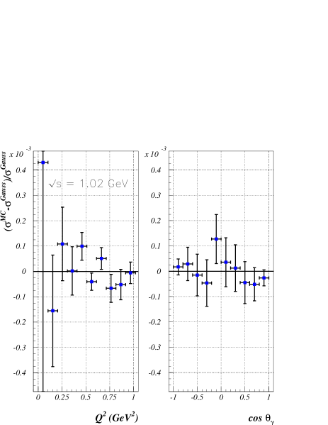
Figure 3: Relative difference between the single photon cross section obtained from the Monte Carlo generator $\sigma^{MC}$ and Gauss quadrature $\sigma^{Gauss}$ (see text for details).

5.2 Soft photon cutoff independence

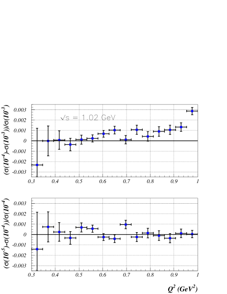
Figure 4: Comparison of the $Q^{2}$ differential distribution for different values of the soft photon cutoff: $w=10^{-3}$, $10^{-4}$ and $10^{-5}$, at $\sqrt{s}=1.02$ GeV.

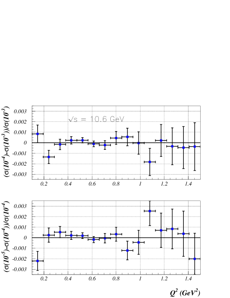
Figure 5: Comparison of the $Q^{2}$ differential distribution for different values of the soft photon cutoff: $w=10^{-3}$, $10^{-4}$ and $10^{-5}$, at $\sqrt{s}=10.6$ GeV.

The full NLO calculation consists of two complementary contributions, the virtual and soft corrections presented in section 2 and the hard correction described in section 3. The former depends logarithmically on the soft photon cutoff $w$, see eq.(7). The second, after numerical integration in phase space exhibits the same behaviour, so that their sum must be independent of $w$.

However, a particular value of $w$ has to be chosen for the generation. To be valid, the soft photon approximation requires $w$ to be small. On the other hand a very small value of $w$ could even produce unphysical negative weights for the generated events. The particular value of $w$ chosen to perform the Monte Carlo generation should therefore arise from a compromise between these two conditions.

In this section we show that the result from the generator is indeed independent from the soft photon cutoff $w$, within the error of the numerical integration. Furthermore, we try to determine the value of $w$ that optimizes the event generation.

Table 1: Kinematical cuts applied at different cms energies: minimal energy of the tagged photon ($E_{\gamma}$), angular cuts on the tagged photon ($\theta_{\gamma}$) and the pions ($\theta_{\pi}$), and minimal invariant mass of the hadrons plus the tagged photon ($M^{2}_{\pi^{+}\pi^{-}\gamma}$)

	$\sqrt{s}=$1.02 GeV	4 GeV	10.6 GeV
$E_{\gamma}^{min}$ (GeV)	$0.01$	$0.1$	$1$
$\theta_{\gamma}$ (degrees)	$[5,21]$	$[10,170]$	$[25,155]$
$\theta_{\pi}$ (degrees)	$[55,125]$	$[20,160]$	$[30,150]$
$M^{2}_{\pi^{+}\pi^{-}\gamma}$ (GeV2)	$0.9$	$12$	$90$

The tests have been performed for different cms energies, from 1 to 10 GeV, corresponding to the energies of DA$\Phi$NE, CLEO-C and $B$-meson factories. Kinematical cuts have been applied as listed in Table 1 and will be used for the rest of the paper. They are related to those of the experiments for which we present our predictions and at the same time allow final state radiation to be controlled, one of the key points of the radiative return method. A minimal energy $E_{\gamma}^{min}$ is required for the tagged photon. Different cuts are chosen for the polar angle of the tagged photon $\theta_{\gamma}$ at different energies. At low energies, the pions are constrained to be well separated from the photons to suppress final state radiation. At high energies, the observed photon and the pions are mainly produced back to back; the suppression of the final state radiation is therefore naturally accomplished. Furthermore, a minimal invariant mass of the hadronic system plus the tagged photon, $M^{2}_{\pi^{+}\pi^{-}\gamma}$, is required. The reason for this last kinematical cut will be discussed later. When events with two photons are simulated we require at least one of the photons to pass the cuts.

Table 2: Total cross section (nb) for the process $e^{+}e^{-}\rightarrow\pi^{+}\pi^{-}\gamma$ at NLO for different values of the soft photon cutoff. Only initial state radiation. Cuts from Table 1.

$w$	$\sqrt{s}=$1.02 GeV	4 GeV	10.6 GeV
$10^{-3}$	2.0324 (4)	0.12524 (5)	0.010564 (4)
$10^{-4}$	2.0332 (5)	0.12526 (5)	0.010565 (4)
$10^{-5}$	2.0333 (5)	0.12527 (5)	0.010565 (5)

Table 2 presents the total cross section calculated for several values of the soft photon cutoff at three different cms energies for the kinematical cuts from Table 1. The excellent agreement confirms the $w$-independence of the result.

Figures 4 and 5 show the $w$-independence of the $Q^{2}$ distribution at $\sqrt{s}=1.02$ GeV and $10.6$ GeV cms energies respectively. Even if the analysis of the total cross section (Table 2) suggests that the choice of $w=10^{-3}$ is as good as $w=10^{-4}$, small differences in the differential cross section are found for high values of $Q^{2}$. Similar comparisons between the differential cross section calculated for $w=10^{-4}$ and $w=10^{-5}$ show a perfect agreement within the statistical errors, well below the 0.1% level. As a result we chose $w=10^{-4}$ for the soft photon cutoff.

5.3 Comparison of NLO results with the structure function approximation and an estimation of the theoretical error

Table 3: Total cross section (nb) for the process $e^{+}e^{-}\rightarrow\pi^{+}\pi^{-}\gamma$ at LO, NLO(1) and in the collinear approximation via structure functions (SF) with the cuts from Table 1. Only initial state radiation. NLO(2) gives the NLO result with the same cuts as NLO(1) but for the hadron–photon invariant mass unbounded.

	$\sqrt{s}=$1.02 GeV	4 GeV	10.6 GeV
Born	2.1361 (4)	0.12979 (3)	0.011350 (3)
SF	2.0192 (4)	0.12439 (5)	0.010526 (3)
NLO (1)	2.0332 (5)	0.12526 (5)	0.010565 (4)
NLO (2)	2.4126 (7)	0.14891 (9)	0.012158 (9)

Table 4: Total cross section (nb) for the process $e^{+}e^{-}\rightarrow\pi^{+}\pi^{-}\gamma$ at $\sqrt{s}=$1.02 GeV in NLO and in the collinear approximation (SF) as a function of the cut on the invariant mass of the hadron + tagged photon $M^{2}_{\pi^{+}\pi^{-}\gamma}$. Only initial state radiation. Minimal energy of the tagged photon and angular cuts from Table 1.

$M^{2}_{\pi^{+}\pi^{-}\gamma}$ (GeV2)	SF	NLO
0.1	2.4127(18)	2.4132(8)
0.2	2.4126(18)	2.4131(8)
0.3	2.4124(18)	2.4127(8)
0.4	2.4098(18)	2.4096(8)
0.5	2.3949(18)	2.3953(8)
0.6	2.3425(16)	2.3455(8)
0.7	2.2449(11)	2.2543(8)
0.8	2.1387(9)	2.1533(8)
0.9	2.0198(8)	2.0334(8)
0.95	1.9437(8)	1.9522(8)
0.99	1.8573(8)	1.8559(8)

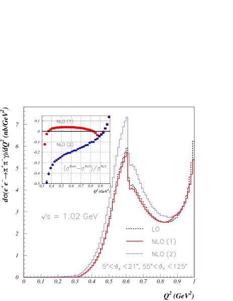
Figure 6: Differential cross section for the process $e^{+}e^{-}\rightarrow\pi^{+}\pi^{-}\gamma$ at NLO for $\sqrt{s}=1.02$ GeV. Only initial state radiation. The relative size of the correction to the LO result (dashed) is shown in the small inset. The cuts are: $5^{\circ}<\theta_{\gamma}<21^{\circ}$, $55^{\circ}<\theta_{\pi}<125^{\circ}$, the energy of the tagged photon $E_{\gamma}>0.01$ GeV and the invariant mass of the detected particles in the final state $M^{2}_{\pi^{+}\pi^{-}\gamma}>0.9$ GeV² for NLO(1) (solid). NLO(2) (dotted) obtained without the last cut.

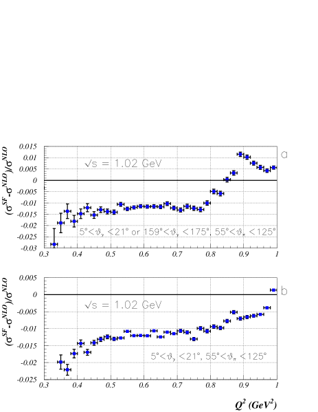
Figure 7: Comparison between the collinear approximation by structure functions and the fixed order NLO result. Cuts from Table 1 for the lower figure. In the upper figure, same cuts as below, with the addition of the symmetric photon configuration $159^{\circ}<\theta_{\gamma}<175^{\circ}$.

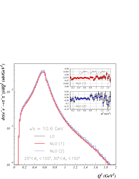
Figure 8: Differential cross section for the process $e^{+}e^{-}\rightarrow\pi^{+}\pi^{-}\gamma$ at NLO for $\sqrt{s}=10.6$ GeV. Only initial state radiation. The relative size of the correction to the LO result (dashed) is shown in the small inset. The cuts are: $25^{\circ}<\theta_{\gamma}<155^{\circ}$, $30^{\circ}<\theta_{\pi}<150^{\circ}$, the energy of the tagged photon $E_{\gamma}>1$ GeV and the invariant mass of the detected particles in the final state $M^{2}_{\pi^{+}\pi^{-}\gamma}>90$ GeV² for NLO(1) (solid). NLO(2) (dotted) obtained without the last cut.

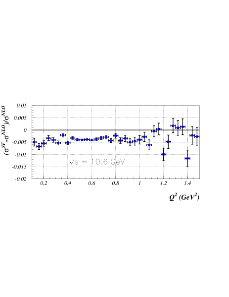
Figure 9: Comparison between the collinear approximation by structure functions and the fixed order NLO result. Cuts from Table 1.

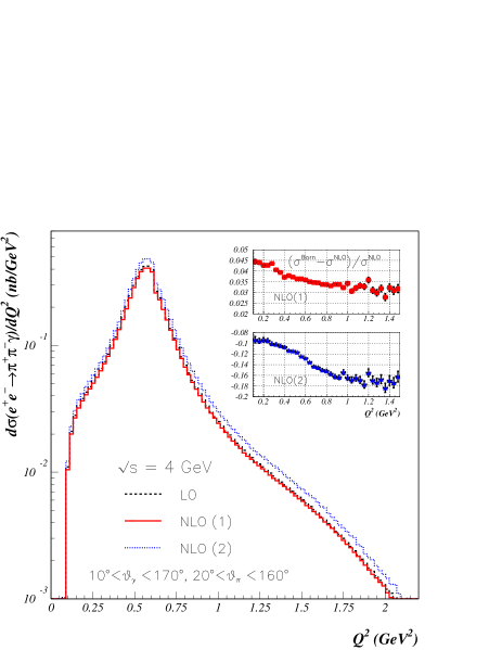
Figure 10: Differential cross section for the process $e^{+}e^{-}\rightarrow\pi^{+}\pi^{-}\gamma$ at NLO for $\sqrt{s}=4$ GeV. Only initial state radiation. The relative size of the correction to the LO result (dashed) is shown in the small inset. The cuts are: $10^{\circ}<\theta_{\gamma}<170^{\circ}$, $20^{\circ}<\theta_{\pi}<160^{\circ}$, the energy of the tagged photon $E_{\gamma}>0.1$ GeV and the invariant mass of the detected particles in the final state $M^{2}_{\pi^{+}\pi^{-}\gamma}>12$ GeV² for NLO(1) (solid). NLO(2) (dotted) obtained without the last cut.

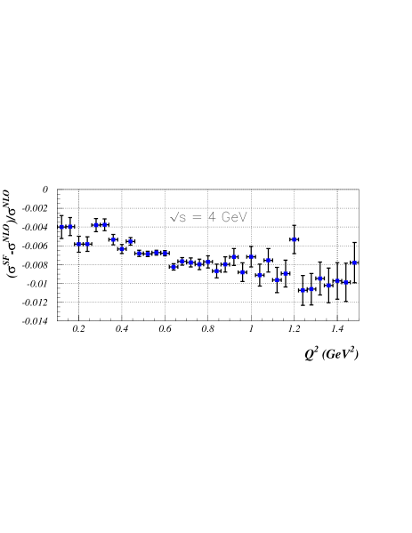
Figure 11: Comparison between the collinear approximation by structure functions and the fixed order NLO result. Cuts from Table 1.

The original and default version of EVA Binner:1999bt , simulating the process $e^{+}e^{-}\rightarrow\pi^{+}\pi^{-}\gamma$ at LO, allowed for additional initial state radiation of soft and collinear photons by the structure function method structure ; Caffo:1997yy . By convoluting the Born cross section with a given SF distribution, the soft photons are resummed to all orders in perturbation theory and large logarithms of collinear origin, $L=\log(s/m_{e}^{2})$, are taken into account up to two-loop approximation. The NLO result, being a complete one-loop result, contains these logarithms in order $\alpha$ and the additional subleading terms, which of course are not taken into account within the SF method. The subleading terms from virtual and soft corrections were calculated in Rodrigo:2001jr and are included in the present NLO generator.

In the SF approach, the additional emission of collinear photons reduces the effective cms energy of the collision. In Binner:1999bt , a minimal invariant mass of the observed particles, hadrons plus tagged photon, was required in order to reduce the kinematic distortion of the events. To perform the comparison between EVA and the present program a similar cut is introduced in the NLO calculation. For one-photon events the invariant mass of the hadrons and the emitted photon is equal to the total cms energy and the requirement is trivially fulfilled. However, when two-photon events are generated, energy and production angles of both photons are compared with the cuts listed in Table 1. If one of the photons fulfils both requirements, its common invariant mass with the hadrons is calculated. In other words, we require at least one of the photons to pass all the cuts, including the one on its common invariant mass with the hadrons. The probability of both photons passing all the cuts becomes very small when this invariant mass cut is close to the total cms energy.

Table 3 gives the total cross section calculated at LO and NLO for the previous kinematical cuts. The soft photon cutoff is fixed at $w=10^{-4}$. For comparison, the total cross section derived from EVA with emission of collinear photons by structure functions Caffo:1997yy ; structure is presented. Two NLO predictions are shown. The first one, NLO(1), which can be compared with the SF result, includes the cut on the invariant mass of the hadrons plus photon. The second one, NLO(2), is obtained without this cut. The results of EVA and those denoted NLO(1) for the total cross section are in agreement to within $0.7\%$. Both of them are clearly sensitive to the cut on $M^{2}_{\pi^{+}\pi^{-}\gamma}$. This cut dependence is displayed in Table 4. Remarkably enough, the typical difference between the results of the two programs is clearly less than $0.5\%$ for most of the entries.

Figure 6 presents our NLO predictions for the differential cross section of the process $e^{+}e^{-}\rightarrow\pi^{+}\pi^{-}\gamma$ as a function of $Q^{2}$, the invariant mass of the hadronic system, at DA$\Phi$NE energies, $\sqrt{s}=1.02$ GeV, with the same kinematical conditions as before. For comparison, also the LO prediction (without collinear emission) is shown, as well as the relative correction. Notice that although the NLO(1) prediction for the total cross section differs from the LO result by roughly $5\%$ (see Table 3), the $Q^{2}$ distribution shows corrections up to $\pm 15\%$ at very low or high values of $Q^{2}$.

As already shown in Table 3 for the total cross section, the invariant mass of the hadron + tagged photon system of a sizeable fraction of events lies below the cut of $0.9$ GeV². These are events where a second hard photon must be present. Including these events leads to the distribution denoted NLO(2) in Fig. 6.

In contrast to the typically $5\%$ difference between LO and NLO(1) predictions, only a $0.6\%$ difference is found between the NLO(1) prediction and the SF collinear approximation as implemented in EVA, this difference being higher at small $Q^{2}$ and lower at high $Q^{2}$, see Fig. 7. As one can see from Fig. 7, the size and sign of the NLO corrections do depend on the particular choice of the experimental cuts. Hence only using a Monte Carlo event generator one can realistically compare theoretical predictions with experiment and extract $R(s)$ from the data. The difference between Figs. 7a and 7b arises from the (small) subset of events with two photons, which both fulfil the angular and energy cuts and thus enter only once in the sample of Fig. 7b.

Results at $10.6$ GeV cms energy are presented in Figs. 8 and 9. In this case a NLO(1) correction to the LO result of $7.5\%$ is found, almost independent of $Q^{2}$, the difference between the NLO(1) prediction and the SF collinear approximation being smaller than $0.5\%$ and also almost independent of $Q^{2}$.

Finally, predictions for $\sqrt{s}=4$ GeV are presented in Figs. 10 and 11.

To estimate the systematic uncertainty of the program, we observe that leading logarithmic two-loop ${\cal O}(\alpha^{2})$ corrections and the associate real emission are not included. The difference between the LO and the NLO(1) results was expected to be of the order of $\frac{3}{2}(\alpha/\pi)\log(s/m_{e}^{2})\approx 5\%$ at $\sqrt{s}=1$ GeV. Indeed one observes (see Fig. 6) values typically of this magnitude with maximal deviations close to $10\%$. From naïve exponentiation one expects $\frac{1}{2}(\frac{3}{2}(\alpha/\pi)\log(s/m_{e}^{2}))^{2}\approx 0.1$–$0.2\%$ for the leading photonic next-to-next-to-leading order (NNLO) terms, which are ignored in the present program.

Another type of $\alpha^{2}$ corrections originates from fermion (dominantly electron) loop insertions in the one-loop virtual corrections considered in Rodrigo:2001jr . These are conveniently combined with the emission of (mainly soft and collinear) real fermions, i.e. with the process $e^{+}e^{-}\rightarrow\gamma\gamma^{*}f\bar{f}$, where the collinear $f\bar{f}$ pair is mostly within the beam pipe and thus undetected. Individually these are corrections of order $(\alpha/\pi)^{2}(\log(s/m_{e}^{2}))^{3}$. When combined, the $\log^{3}(s/m_{e}^{2})$ terms cancel and the remaining $\frac{1}{4}(\alpha/\pi)^{2}(\log(s/m_{e}^{2}))^{2}$ term can be largely absorbed by choosing a running coupling $\alpha$(1 GeV) in the NLO terms and thus amount to less than $0.1\%$. Adding these contributions linearly, one estimates a $0.3\%$ uncertainty .

Multiphoton emission is not included in the present program. In an inclusive treatment and for tight cuts on the photon energy, this can in principle be included through exponentiation. For the cuts on $M^{2}_{\pi^{+}\pi^{-}\gamma}$ of $0.9$ GeV² proposed originally in Binner:1999bt , and adopted through most of this paper, the difference between the exponentiated form and the fixed order treatment (see e.g. eqs. 17 and 19 of Rodrigo:2001jr ) amounts to roughly $0.7\%$, with smaller values for less restrictive cuts. For a cut of $M^{2}_{\pi^{+}\pi^{-}\gamma}$ at $0.8$ GeV² or even $0.7$ GeV², which seems preferable from these considerations, we expect a difference of $0.4\%$ and even below $0.3\%$ for the second choice. In total we therefore estimate a systematic uncertainty from ISR of around $0.5\%$ in the total cross section, once loose cuts on $M^{2}_{\pi^{+}\pi^{-}\gamma}$ are adopted. FSR can be controlled by suitable cuts or corrected with the Monte Carlo program EVA.

5.4 Muon pair production

Inclusion of muon production in the program is straightforward. The results for the total cross section are listed in Table 5, the differential distributions for the three cms energies in Figs. 12 – 14. The radiative muon cross section could be used for a calibration of the pion yield. A number of radiative corrections are expected to cancel in the ratio. For this reason we consider the ratio between the pion and the muon yields, after dividing the former by $|F_{\pi}(Q^{2})|^{2}(1-4m_{\pi}^{2}/Q^{2})^{3/2}$, the latter by $4(1+2m_{\mu}^{2}/Q^{2})\sqrt{1-4m_{\mu}^{2}/Q^{2}}$. In Fig. 15a we consider the full angular range for pions and muons, with $\theta_{\gamma}$ between $5^{\circ}$ and $21^{\circ}$. Clearly all radiative corrections and kinematic effects disappear, up to statistical fluctuations, in the leading order program as well as after inclusion of the NLO corrections.

In Fig. 15b an additional cut on pion and muon angles has been imposed. As demonstrated in Fig. 15b, the ratio differs from unity once (identical) angular cuts are imposed on pions and muons, a consequence of their different respective angular distribution. To derive the pion form factor from the ratio between pion and muon yields, this effect has to be incorporated. However, the correction function shown in Fig. 15b is independent from the form factor, and hence universal. It can be obtained from the present program in a model-independent way (ignoring FSR for the moment).

Table 5: Total cross section (nb) for initial state radiation in the process $e^{+}e^{-}\rightarrow\mu^{+}\mu^{-}\gamma$ at LO, NLO (1) and NLO (2) with the cuts from Table 1, the pions being replaced by muons.

	$\sqrt{s}=$1.02 GeV	4 GeV	10.6 GeV
Born	0.8243(5)	0.4690(6)	0.003088(6)
NLO (1)	0.7587(5)	0.4449(6)	0.002865(6)
NLO (2)	0.8338(7)	0.4874(14)	0.00321(6)

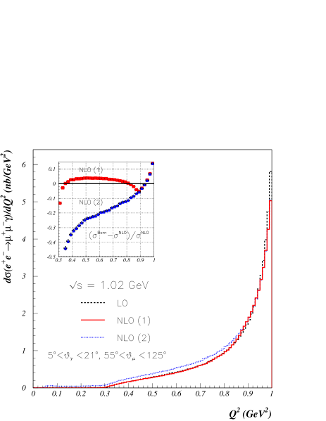
Figure 12: Differential cross section for the process $e^{+}e^{-}\rightarrow\mu^{+}\mu^{-}\gamma$ at NLO for $\sqrt{s}=1.02$ GeV. Only initial state radiation. The relative size of the correction to the LO result (dashed) is shown in the small inset. Same cuts as in figure 6, with the pions replaced by muons.

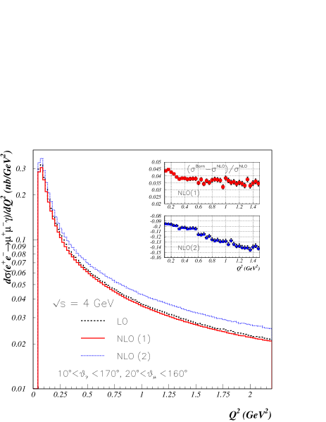
Figure 13: Differential cross section for the process $e^{+}e^{-}\rightarrow\mu^{+}\mu^{-}\gamma$ at NLO for $\sqrt{s}=4$ GeV. Only initial state radiation. The relative size of the correction to the LO result (dashed) is shown in the small inset. Same cuts as in Fig. 10, with the pions replaced by muons.

Figure 14: Differential cross section for the process $e^{+}e^{-}\rightarrow\mu^{+}\mu^{-}\gamma$ at NLO for $\sqrt{s}=10.6$ GeV. Only initial state radiation. The relative size of the correction to the LO result (dashed) is shown in the small inset. Same cuts as in Fig. 8, with the pions replaced by muons.

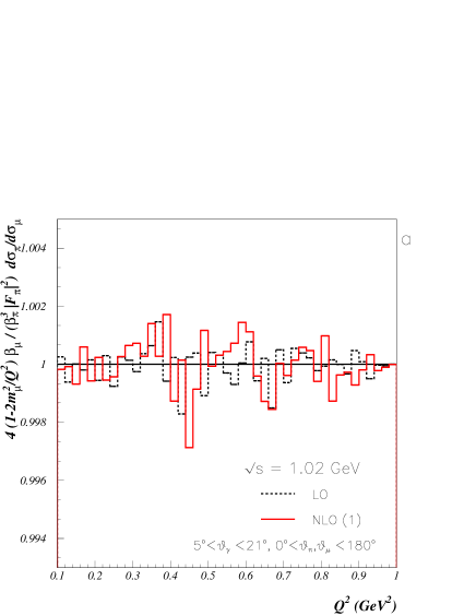
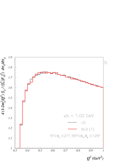
Figure 15: Ratio between pion and muon yields, after dividing through their respective R-ratio. Fig. a: no cuts on pion and muon angles. Fig. b: with angular cuts on pion and muon angles.

6 Conclusions

The radiative return with tagged photons offers a unique opportunity for a measurement of $\sigma(e^{+}e^{-}\rightarrow hadrons)$ over a wide range of energies. The reduction of the cross section by the additional factor $\alpha/\pi$ is easily compensated by the high luminosity of the new $e^{+}e^{-}$ colliders, specifically the $\phi$-, charm- and $B$-factories at Frascati, Cornell, Stanford and KEK.

In the present work we presented a Monte Carlo generator that simulates this reaction to next-to-leading accuracy. The current version includes initial state radiation only and is limited to $\pi^{+}\pi^{-}\gamma(\gamma)$ and $\mu^{+}\mu^{-}\gamma(\gamma)$ as final states. The uncertainty from unaccounted higher order ISR is estimated at around $0.5\%$. The dominant FSR contribution can be deduced from the earlier program EVA. Additional hadronic modes can be easily implemented in the present program. The modes with three and four pions are in preparation.

Appendix A Helicity amplitudes

In this appendix the full set of helicity amplitudes for the diagrams of Fig. 2 is given. Notation and calculation procedure were outlined in section 3, which follows Refs. Jegerlehner:2000wu ; Kolodziej:1991pk .

As an example, consider the amplitude of the first Feynman diagram in Fig. 2:

$$M_{1} =T_{1}^{\mu}J_{\mu}=\frac{e^{3}}{Q^{2}}\bar{v}(p_{1})\varepsilon/^{*}(k_{1})[k/_{1}-p/_{1}+m_{e}]$$

$$\times\varepsilon/^{*}(k_{2})[k/_{1}+k/_{2}-p/_{1}+m_{e}]\gamma^{\mu}u(p_{2})J_{\mu}$$

$$\times\frac{1}{(2k_{1}\cdot p_{1})(2k_{1}\cdot k_{2}-2k_{1}\cdot p_{1}-2k_{2}\cdot p_{1})}~{}.$$ (41)

Using the Dirac equation, after some algebra, the following expression is obtained

$$M_{1} =\frac{e^{3}}{Q^{2}}\bigg{(}v_{I}^{\dagger}(p_{1})[\varepsilon^{*}(k_{1})^{-}k_{1}^{+}-2\varepsilon^{*}(k_{1})\cdot p_{1}]$$

$$\times\varepsilon^{*}(k_{2})^{-}[2p_{2}\cdot J-Q^{+}J^{-}]u_{I}(p_{2})$$

$$+v_{II}^{\dagger}(p_{1})[\varepsilon^{*}(k_{1})^{+}k_{1}^{-}-2\varepsilon^{*}(k_{1})\cdot p_{1}]$$

$$\times\varepsilon^{*}(k_{2})^{+}[2p_{2}\cdot J-Q^{-}J^{+}]u_{II}(p_{2})\bigg{)}$$

$$\times\frac{1}{(2k_{1}\cdot p_{1})(2k_{1}\cdot k_{2}-2k_{1}\cdot p_{1}-2k_{2}\cdot p_{1})}~{}.$$ (42)

Similar expressions are found for the amplitudes of the other diagrams and the complete matrix element can be written in a simple form (38), where the matrices $A\left(\lambda_{1},\lambda_{2}\right)$ and $B\left(\lambda_{1},\lambda_{2}\right)$ are defined as:

$$A = -\frac{e^{3}}{4Q^{2}}\biggl{(}\frac{a_{1}a_{3}}{(k_{2}\cdot p_{1})N_{1}}+\frac{a_{5}a_{3}}{(k_{1}\cdot p_{1})N_{1}}+\frac{a_{5}a_{7}}{(k_{1}\cdot p_{1})(k_{2}\cdot p_{2})}$$

$$+\frac{a_{1}a_{9}}{(k_{2}\cdot p_{1})(k_{1}\cdot p_{2})}+\frac{a_{11}a_{7}}{(k_{2}\cdot p_{2})N_{2}}+\frac{a_{11}a_{9}}{(k_{1}\cdot p_{2})N_{2}}\biggr{)}\ ,$$

$$B = -\frac{e^{3}}{4Q^{2}}\biggl{(}\frac{a_{2}a_{4}}{(k_{2}\cdot p_{1})N_{1}}+\frac{a_{6}a_{4}}{(k_{1}\cdot p_{1})N_{1}}+\frac{a_{6}a_{8}}{(k_{1}\cdot p_{1})(k_{2}\cdot p_{2})}$$

$$+\frac{a_{2}a_{10}}{(k_{2}\cdot p_{1})(k_{1}\cdot p_{2})}+\frac{a_{12}a_{8}}{(k_{2}\cdot p_{2})N_{2}}+\frac{a_{12}a_{10}}{(k_{1}\cdot p_{2})N_{2}}\biggr{)}\ \ ,$$

where

$$N_{1} = k_{1}\cdot p_{1}+k_{2}\cdot p_{1}-k_{1}\cdot k_{2}~{},$$

$$N_{2} = k_{1}\cdot p_{2}+k_{2}\cdot p_{2}-k_{1}\cdot k_{2}~{},$$

$$a_{1} = \varepsilon^{*}(k_{2})^{-}k_{2}^{+}-2\varepsilon^{*}(k_{2})\cdot p_{1}~{},$$

$$a_{2} = \varepsilon^{*}(k_{2})^{+}k_{2}^{-}-2\varepsilon^{*}(k_{2})\cdot p_{1}~{},$$

$$a_{3} = 2p_{2}\cdot J-Q^{+}J^{-}~{},$$

$$a_{4} = 2p_{2}\cdot J-Q^{-}J^{+}~{},$$

$$a_{5} = \varepsilon^{*}(k_{1})^{-}k_{1}^{+}-2\varepsilon^{*}(k_{1})\cdot p_{1}~{},$$

$$a_{6} = \varepsilon^{*}(k_{1})^{+}k_{1}^{-}-2\varepsilon^{*}(k_{1})\cdot p_{1}~{},$$

$$a_{7} = 2\varepsilon^{*}(k_{2})\cdot p_{2}-k_{2}^{+}\varepsilon^{*}(k_{2})^{-}~{},$$

$$a_{8} = 2\varepsilon^{*}(k_{2})\cdot p_{2}-k_{2}^{-}\varepsilon^{*}(k_{2})^{+}~{},$$

$$a_{9} = 2\varepsilon^{*}(k_{1})\cdot p_{2}-k_{1}^{+}\varepsilon^{*}(k_{1})^{-}~{},$$

$$a_{10} = 2\varepsilon^{*}(k_{1})\cdot p_{2}-k_{1}^{-}\varepsilon^{*}(k_{1})^{+}~{},$$

$$a_{11} = J^{-}Q^{+}-2p_{1}\cdot J~{},$$

$$a_{12} = J^{+}Q^{-}-2p_{1}\cdot J~{}.$$

The current $J^{\mu}$ is defined by the eq.(4) for the $\pi^{+}\pi^{-}$ final state, while for the $\mu^{+}\mu^{-}$ one it is defined as follows:

$$J^{\mu}(\lambda_{1},\lambda_{2})=ie\bar{u}(q_{1},\lambda_{1})\gamma^{\mu}v(q_{2},\lambda_{2})\ \ ,$$ (45)

where $q_{1},\lambda_{1}$ ($q_{2},\lambda_{2}$) are four-momentum and helicity of $\mu^{-}$ ($\mu^{+}$).

Appendix B Phase space

The generation of the multiparticle phase space is based on the following Lorentz-invariant representation:

$$d\Phi_{m+n}(p_{1},p_{2};k_{1},\cdot,k_{m},q_{1},\cdot,q_{n})=$$

$$\qquad d\Phi_{m}(p_{1},p_{2};Q,k_{1},\cdot,k_{m})d\Phi_{n}(Q;q_{1},\cdot,q_{n})\frac{dQ^{2}}{2\pi}~{},$$ (46)

where $p_{1}$ and $p_{2}$ are the four-momenta of the initial particles, $k_{1}\ldots k_{m}$ are the four momenta of the emitted photons and $q_{1}\ldots q_{n}$, with $Q=\sum q_{i}$, label the four-momenta of the hadrons.

When two pions are produced in the final state, the hadronic part of phase space is given by

$$d\Phi_{2}(Q;q_{1},q_{2})=\frac{\sqrt{1-\frac{4m_{\pi}^{2}}{Q^{2}}}}{32\pi^{2}}d\Omega~{},$$ (47)

where $d\Omega$ is the solid angle of one of the pions at, for instance, the $Q^{2}$ rest frame.

One single photon emission is described by the corresponding leptonic part of phase space

$$d\Phi_{2}(p_{1},p_{2};Q,k_{1})=\frac{1-q^{2}}{32\pi^{2}}d\Omega_{1}~{},$$ (48)

with $q^{2}=Q^{2}/s$ and $d\Omega_{1}$ is the solid angle of the emitted photon at the $e^{+}e^{-}$ rest frame. The polar angle $\theta_{1}$ is defined with respect to the positron momentum $p_{1}$. In order to make the Monte Carlo generation more efficient, the following substitution is performed:

$$\cos\theta_{1}=\frac{1}{\beta}\tanh(\beta\;t_{1})~{},\quad t_{1}=\frac{1}{2\beta}\log\frac{1+\beta\cos\theta_{1}}{1-\beta\cos\theta_{1}}~{},$$ (49)

with $\beta=\sqrt{1-4m_{e}^{2}/s}$, which accounts for the collinear emission peaks

$$\frac{d\cos\theta_{1}}{1-\beta^{2}\cos^{2}\theta_{1}}=dt_{1}~{}.$$ (50)

Then, the azimuthal angle and the new variable $t_{1}$ are generated flat.

Consider now the emission of two real photons. In the cms of the initial particles, the four-momenta of the positron, the electron and the two emitted photons are given by

$$p_{1} =\frac{\sqrt{s}}{2}(1,0,0,\beta)~{},\qquad p_{2}=\frac{\sqrt{s}}{2}(1,0,0,-\beta)~{},$$

$$k_{1} =w_{1}\sqrt{s}(1,\sin\theta_{1}\cos\phi_{1},\sin\theta_{1}\sin\phi_{1},\cos\theta_{1})~{},$$

$$k_{2} =w_{2}\sqrt{s}(1,\sin\theta_{2}\cos\phi_{2},\sin\theta_{2}\sin\phi_{2},\cos\theta_{2})~{},$$ (51)

respectively. The polar angles $\theta_{1}$ and $\theta_{2}$ are defined again with respect to the positron momentum $p_{1}$. Both photons are generated with energies larger than the soft photon cutoff: $w_{i}>w$ with $i=1,2$. At least one of these should exceed the minimal detection energy: $w_{1}>E_{\gamma}^{min}/s$ or $w_{2}>E_{\gamma}^{min}/s$. In terms of the solid angles $d\Omega_{1}$ and $d\Omega_{2}$ of the two photons and the normalized energy of one of them, e.g. $w_{1}$, the leptonic part of phase space reads

$$d\Phi_{3}(p_{1},p_{2};Q,k_{1},k_{2}) =\frac{1}{2!}\;\frac{s}{4(2\pi)^{5}}$$

$$\times \frac{w_{1}w_{2}^{2}}{1-q^{2}-2w_{1}}\;dw_{1}\;d\Omega_{1}\;d\Omega_{2}~{},$$ (52)

where the limits of the phase space are defined by the constraint

$$q^{2}=1-2(w_{1}+w_{2})+2w_{1}w_{2}(1-\cos\chi_{12})~{},$$ (53)

with $\chi_{12}$ being the angle between the two photons

$$\cos\chi_{12}=\sin\theta_{1}\sin\theta_{2}\cos(\phi_{1}-\phi_{2})+\cos\theta_{1}\cos\theta_{2}~{}.$$ (54)

Again, the matrix element squared contains several peaks, soft and collinear, which should be softened by choosing suitable substitutions in order to achieve an efficient Monte Carlo generator. The leading behaviour of the matrix element squared is given by $1/(y_{11}\;y_{12}\;y_{21}\;y_{22})$, where

$$y_{ij}=\frac{2k_{i}\cdot p_{j}}{s}=w_{i}(1\mp\beta\cos\theta_{i})~{}.$$ (55)

In combination with the leptonic part of phase space, we have

$$\frac{d\Phi_{3}(p_{1},p_{2};Q,k_{1},k_{2})}{y_{11}\;y_{12}\;y_{21}\;y_{22}}\sim\frac{dw_{1}}{w_{1}(1-q^{2}-2w_{1})}\;$$

$$\qquad\times\frac{d\Omega_{1}}{1-\beta^{2}\cos^{2}{\theta_{1}}}\;\frac{d\Omega_{2}}{1-\beta^{2}\cos^{2}{\theta_{2}}}~{}.$$ (56)

The collinear peaks are then flattened with the help of eq.(49), with one change of variables for each photon polar angle. The remaining soft peak, $w_{1}\rightarrow w$, is reabsorbed with the following substitution

$$w_{1}=\frac{1-q^{2}}{2+e^{-u_{1}}}~{},\quad u_{1}=\log\frac{w_{1}}{1-q^{2}-2w_{1}}~{},$$ (57)

or

$$\frac{dw_{1}}{w_{1}(1-q^{2}-2w_{1})}=\frac{du_{1}}{1-q^{2}}~{},$$ (58)

where the new variable $u_{1}$ is generated flat.

References

- (1) H. N. Brown et al. [Muon Collaboration], Phys. Rev. Lett. 86 (2001) 2227 [hep-ex/0102017].
- (2) V. W. Hughes and T. Kinoshita, Rev. Mod. Phys. 71 (1999) S133.
- (3) S. Eidelman and F. Jegerlehner, Z. Phys. C 67 (1995) 585 [hep-ph/9502298]. D. H. Brown and W. A. Worstell, Phys. Rev. D 54 (1996) 3237 [hep-ph/9607319]. M. Davier and A. Höcker, Phys. Lett. B 435 (1998) 427 [hep-ph/9805470]. S. Narison, Phys. Lett. B 513 (2001) 53 [hep-ph/0103199]. F. Jegerlehner, [hep-ph/0104304]. J. F. De Trocóniz and F. J. Ynduráin, [hep-ph/0106025].
- (4) H. Burkhardt and B. Pietrzyk, Phys. Lett. B 513 (2001) 46. A. D. Martin, J. Outhwaite and M. G. Ryskin, [hep-ph/0012231]; Phys. Lett. B 492 (2000) 69 [hep-ph/0008078]. J. Erler, Phys. Rev. D 59 (1999) 054008 [hep-ph/9803453]. J. H. Kühn and M. Steinhauser, [hep-ph/0109084]; Phys. Lett. B 437 (1998) 425 [hep-ph/9802241].
- (5) S. Binner, J. H. Kühn and K. Melnikov, Phys. Lett. B459 (1999) 279 [hep-ph/9902399].
- (6) K. Melnikov, F. Nguyen, B. Valeriani and G. Venanzoni, Phys. Lett. B477 (2000) 114 [hep-ph/0001064].
- (7) H. Czyż and J. H. Kühn, Eur. Phys. J. C 18 (2001) 497 [hep-ph/0008262].
- (8) S. Spagnolo, Eur. Phys. J. C 6 (1999) 637.
- (9) V. A. Khoze, M. I. Konchatnij, N. P. Merenkov, G. Pancheri, L. Trentadue and O. N. Shekhovzova, Eur. Phys. J. C 18 (2001) 481 [hep-ph/0003313].
- (10) R. R. Akhmetshin et al. [CMD-2 Collaboration], [hep-ex/9904027].
- (11) A. Höfer, J. Gluza and F. Jegerlehner, [hep-ph/0107154].
- (12) A. Aloisio et al. [KLOE Collaboration], [hep-ex/0107023].
- (13) A. Denig et al. [KLOE Collaboration], eConf C010430 (2001) T07 [hep-ex/0106100].
- (14) M. Adinolfi et al. [KLOE Collaboration], [hep-ex/0006036].
- (15) E. P. Solodov [BABAR collaboration], eConf C010430 (2001) T03 [hep-ex/0107027].
- (16) G. Rodrigo, A. Gehrmann-De Ridder, M. Guilleaume and J. H. Kühn, Eur. Phys. J. C 22 (2001) 81 [hep-ph/0106132].
- (17) G. Rodrigo, Acta Phys. Polon. B 32 (2001) 3833 [hep-ph/0111151].
- (18) J. H. Kühn and A. Santamaria, Z. Phys. C 48 (1990) 445.
- (19) M. Böhm, H. Spiesberger and W. Hollik, Fortsch. Phys. 34 (1986) 687.
- (20) F. Jegerlehner and K. Kołodziej, Eur. Phys. J. C 12 (2000) 77 [hep-ph/9907229].
- (21) K. Kołodziej and M. Zrałek, Phys. Rev. D 43 (1991) 3619.
- (22) E. A. Kuraev and V. S. Fadin, Sov. J. Nucl. Phys. 41 (1985) 466. G. Altarelli and G. Martinelli, in Physics at LEP, CERN Report 86-06, eds. J. Ellis and R. Peccei (CERN, Geneva, February 1986). O. Nicrosini and L. Trentadue, Phys. Lett. B196 (1987) 551.
- (23) M. Caffo, H. Czyż and E. Remiddi, Nuovo Cim. A 110 (1997) 515 [hep-ph/9704443]; Phys. Lett. B327 (1994) 369.
- (24) B. A. Kniehl, M. Krawczyk, J. H. Kühn and R. G. Stuart, Phys. Lett. B 209 (1988) 337.