CORRECTIONS TO FERMI’S GOLDEN RULE IN $\phi\rightarrow K\bar{K}$ DECAYS

E. Fischbach^(a), A.W. Overhauser^(a), and B. Woodahl^(b,a)

Abstract

We analyze the decays $\phi\rightarrow K\bar{K}$ utilizing a formulation of transition rates which explicitly exhibits corrections to Fermi’s Golden Rule. These corrections arise in systems in which the phase space and/or matrix element varies rapidly with energy, as happens in $\phi\rightarrow K\bar{K}$, which is just above threshold. We show that the theoretical corrections resolve a puzzling $5\sigma$ discrepancy between theory and experiment for the branching ratio $R=\Gamma(\phi\rightarrow K^{+}K^{-})/\Gamma(\phi\rightarrow K^{0}\bar{K}^{0})$.

One of the most well known results from elementary quantum mechanics is the formula relating the rate $\Gamma$ for the transition $|i>\rightarrow|n>$ to the matrix element $V_{ni}(E)\equiv<n|V|i>$ induced by a time-independent perturbation $V$,

$$\Gamma(i\rightarrow n)=\frac{2\pi}{\hbar}|V_{ni}(E)|^{2}\rho(E),$$

where $E=E_{n}-E_{i}$, and $\rho(E)=dN/dE$ is the energy density of the final states $n$ [1]. This formula is so useful and so widely applied that Fermi named it “Golden Rule No. 2” (FGR2) [2]. As almost all derivations of Eq.(1) make clear, FGR2 is an approximation which is valid in the limit when both $|V_{ni}(E)|^{2}$ and $\rho(E)$ are “slowly varying” functions of $E$, although the precise meaning of “slowly varying” is not always made explicit. However, it is evident that $|V_{ni}(E)|^{2}\rho(E)$ will not be slowly varying in some circumstances, for example, when the initial state $|i>$ is just above the threshold for decay into the final state $|n>$. This is the case for the decays $\phi\rightarrow K\bar{K}$ (either $\phi\rightarrow K^{+}K^{-}$ or $\phi\rightarrow K^{0}\bar{K}^{0})$, where $m_{\phi}=1019.417(14)MeV$, while $m_{K^{+}}=493.677(16)MeV$, and $m_{K^{0}}=497.672(31)MeV$ [3]. Quark model diagrams for these decays are shown in Fig. 1. In principle the corrections to FGR2 in such decays could be large enough to lead to detectable effects, and in what follows we show that this is in fact the case. More interestingly, we demonstrate explicitly that the correction to FGR2 arising from the rapid variation of $|V_{ni}(E)|^{2}\rho(E)$ with $E$ resolves a puzzling discrepancy [5] between theory and experiment for the ratio $R=\Gamma(\phi\rightarrow K^{+}K^{-})/\Gamma(\phi\rightarrow K^{0}\bar{K}^{0})$.

An explicit expression for the corrections to FGR2 can be conveniently derived by endowing the initial decaying state at the outset with a lifetime $\tau=1/\Gamma$, and then solving self-consistently for $\Gamma$. Consider an initial state $|i,t_{0}>$ which evolves into the state $|i,t>$ at a later time $t$ under the influence of the time evolution operator $U(t,t_{0})$. The state $|i,t>$ can be expanded in terms of a complete set of eigenfunctions $|n>$ of the unperturbed Hamiltonian,

$$\begin{array}[]{rcl}|i,t>&=&\sum_{n}|n><n|U(t,t_{0})|i,t_{0}>\equiv\sum_{n}c_{n}(t)|n>,\\ &{}\hfil&\\ c_{n}(t)&=&\frac{-i}{\hbar}\int_{t_{0}}^{t}dt^{\prime}e^{i\omega_{ni}t^{\prime}}e^{-\Gamma t^{\prime}/2}V_{ni},\end{array}$$

where $\hbar\omega_{ni}=E_{n}-E_{i}$, and $E_{i}(E_{n})$ is the unperturbed initial (final) energy. Without loss of generality we can set $t_{0}=0$, the instant at which the $\phi$ is produced. The quantity of interest is $c_{n}{(\infty)}$ which is given by

$$c_{n}({\infty})=\frac{-i}{\hbar}\int_{0}^{\infty}dt^{\prime}e^{(i\omega_{ni}-\Gamma/2)t^{\prime}}V_{ni}=\frac{i}{\hbar}V_{ni}\frac{1}{i\omega_{ni}-\Gamma/2},$$

where $V_{ni}$ is independent of time. We next impose the unitarity constraint on $c_{n}({\infty})$, namely $\sum_{n}|c_{n}({\displaystyle{\infty}})|^{2}=1$. After the sum is converted into an integral in the usual manner, $\sum_{n}\rightarrow\int dE\rho(E)$, the unitarity constraint assumes the form

$$1=\int_{-\infty}^{\infty}dE\rho(E)\frac{|V(E)|^{2}}{E^{2}+(\hbar\Gamma/2)^{2}}~{}~{}~{},$$

where we have set $\hbar\omega_{ni}\rightarrow E$, and $V_{ni}\rightarrow V(E)$. The denominator in Eq.(4) is rapidly varying in the vicinity of $E\equiv E_{0}\cong 0$, which corresponds to an energy-conserving transition. Thus if we invoke the assumption that $\rho(E)|V(E)|^{2}$ is slowly varying with respect to the denominator [$E^{2}+(\hbar\Gamma/2)^{2}]$, then the unitarity constraint in Eq.(4) yields

$$1\cong\rho(E_{0})|V(E_{0})|^{2}\int_{-\infty}^{\infty}dE\frac{1}{E^{2}+(\hbar\Gamma/2)^{2}}=\rho(E_{0})|V(E_{0})|^{2}\cdot(2\pi/\hbar\Gamma).$$

Solving Eq.(5) for $\Gamma$ we are led immediately to the standard Fermi Golden Rule in Eq.(1). Moreover, the Golden Rule integral technique (GRIT) embodied in Eq.(4) gives a specific formula for the corrections to FGR2 in Eq.(1) for processes in which $\rho(E)$ and/or $|V(E)|^{2}$ varies significantly with energy. One can further elucidate the approximation being made in going from Eq.(4) to Eq.(5) by invoking the identity

$$\lim_{\alpha\rightarrow 0}\frac{1}{E^{2}+\alpha^{2}}=\frac{\pi}{\alpha}\delta(E),$$

where $\alpha=\hbar\Gamma/2$. Combining Eqs.(4) and (6) leads immediately to Eq.(5) in the limit $\Gamma\rightarrow 0$. However, for $\Gamma\not=0$ $\delta(E)$ is replaced by the (broader) Lorentzian in Eq.(4) which introduces contributions from $\rho(E)|V(E)|^{2}$ in which $E\not=0$. As we now demonstrate, these additional contributions are quantitatively different for $\phi\rightarrow K^{+}K^{-}$ and $\phi\rightarrow K^{0}\bar{K}^{0}$, and their inclusion serves to resolve a $5\sigma$ discrepancy between the theoretical and experimental values [4,5] of $R=\Gamma(\phi\rightarrow K^{+}K^{-})/\Gamma(\phi\rightarrow K^{0}\bar{K}^{0}$).

The decay $\phi\rightarrow K^{+}K^{-}$ is induced by the Lagrangian density

$${\cal{L}}(x)=ig_{+}\phi^{\mu}(x)[K^{+}(x)\partial_{\mu}K^{-}(x)-K^{-}(x)\partial_{\mu}K^{+}(x)],$$

where $g_{+}$ is the appropriate coupling constant, and $K^{+}(x)$ annihilates $K^{+}$, etc. A similar expression characterizes $\phi\rightarrow K^{0}\bar{K}^{0}$, which is proportional to the coupling constant $g_{0}$, with $g_{0}=g_{+}$ in the limit of exact SU(2) symmetry. Bramon, et al. [5] have considered the effects of radiative corrections, and we will return to their results below. Using FGR2 as given in Eq.(1) the decay rate $\Gamma(\phi\rightarrow K^{+}K^{-})$ obtained from Eq.(7) is given by (setting $\hbar=c=1$ hereafter),

$$\Gamma(\phi\rightarrow K^{+}K^{-})=\frac{2}{3}\left(\frac{g_{+}^{2}}{4\pi}\right)\frac{|\vec{k}|^{3}}{m_{\phi}^{2}},$$

where $|\vec{k}|=(1/2)(m_{\phi}^{2}-4m_{K^{+}}^{2})^{1/2}$ is the magnitude of the $K^{+}$ 3-momentum in the $\phi$ rest frame. The factor of $|\vec{k}|^{3}$ can be understood as follows: Since the kaons are spinless, whereas $\phi$ is a vector particle, angular momentum conservation demands that $K$ and $\bar{K}$ be emitted in a relative $P-$wave, which is consistent with the derivative coupling in Eq.(7). Hence $|$$<V_{ni}>$$|^{2}$ contributes a factor of $|\vec{k}|^{2}$, while the phase space contributes an additional factor $dN/dE\propto|\vec{k}|$. Combining Eq.(8) with the corresponding expression for $\phi\rightarrow K^{0}\bar{K}^{0}$ we find using FGR2,

$$R_{th}\equiv\frac{\Gamma(\phi\rightarrow K^{+}K^{-})}{\Gamma(\phi\rightarrow K^{0}\bar{K}^{0})}\Biggr{|}_{th}\equiv\left(\frac{g_{+}^{2}}{g_{0}^{2}}\right)R_{FGR2}=\left(\frac{g_{+}^{2}}{g_{0}^{2}}\right)\left(\frac{1-4\mu_{+}^{2}}{1-4\mu_{0}^{2}}\right)^{3/2},$$

where $\mu_{+}=m_{K^{+}}/m_{\phi}$ and $\mu_{0}=m_{K^{0}}/m_{\phi}$. Inserting the previously quoted values of $m_{K^{+}},m_{K^{0}}$, and $m_{\phi}$ into Eq.(9), and assuming $g_{0}=g_{+}$, we find $R_{th}=1.528$, to be compared with the experimental value [4]

$$R_{exp}=1.456\pm 0.033~{}~{}~{}.$$

Bramon, et al. [5] have evaluated various corrections to $R_{th}$ in an effort to bring $R_{th}$ and $R_{exp}$ into agreement. Most significant among these are electromagnetic radiative corrections which affect $\phi\rightarrow K^{+}K^{-}$ but not $\phi\rightarrow K^{0}\bar{K}^{0}$. These authors find that the radiative correction factor, $\eta=1.042$, increases $R_{th}$ to 1.59. Bramon et al. have also studied the effects of SU(2) symmetry breaking on the ratio $g_{+}/g_{0}$, which arise via quark mass differences. The $\phi$ wavefunction is pure $s\bar{s}$, and hence the $K^{+}K^{-}$ $(K^{0}\bar{K}^{0})$ final state requires the creation of an additional $u\bar{u}(d\bar{d})$ pair (see Fig. 1). Since the $u\bar{u}$ pair is lighter than $d\bar{d}$, one expects this effect to enhance $\phi\rightarrow K^{+}K^{-}$ relative to $\phi\rightarrow K^{0}\bar{K}^{0}$, thus further widening the discrepancy between theory and experiment. A detailed analysis by Bramon et al. [5] finds $g_{+}/g_{0}\cong 1.01$, which agrees with the intuitive expectation that this correction also works in the wrong direction. With this correction included $R_{th}$ becomes 1.62. Other effects considered by these authors, such as the inclusion of electromagnetic form factors in calculating radiative corrections, and final-state rescattering effects, are negligible. We are thus left with a puzzling $5\sigma$ discrepancy between $R_{th}=1.62$ and $R_{exp}=1.456~{}(33)$.

We proceed to demonstrate that this discrepancy can be resolved by incorporating the corrections to FGR2 that arise from the Golden Rule integral technique. Combining Eqs.(4) and (8), and introducing the notation $z=E/m_{\phi}$, $a=\Gamma/2m_{\phi}$, $(\Gamma=4.458(32)$MeV) we express the unitarity constraint for $\phi$-decays in the form,

$$\begin{array}[]{rcl}1&=&\frac{1}{3\pi}\left(\frac{g_{+}^{2}}{4\pi}\right)\int\frac{dz}{(1+z)}\frac{1}{z^{2}+a^{2}}\left[\frac{1}{4}(1+z)^{2}-\mu_{+}^{2}\right]^{3/2}\\ &&\\ &+&\frac{1}{3\pi}\left(\frac{g_{0}^{2}}{4\pi}\right)\int\frac{dz}{(1+z)}\frac{1}{z^{2}+a^{2}}\left[\frac{1}{4}(1+z)^{2}-\mu_{0}^{2}\right]^{3/2}~{}~{}+...~{}~{}~{}~{}.\end{array}$$

The two terms exhibited in Eq.(11) are, respectively, the contributions from the $K^{+}K^{-}$ and $K^{0}\bar{K}^{0}$ states, and $...$ denotes contributions to the unitarity integral from other channels (such as $\rho\pi)$ which can be ignored for present purposes. We emphasize that the functional form of the expressions in square-brackets in Eq.(11) is determined by the kinematics of $\phi\rightarrow K\bar{K}$, specifically by the relation between $|\vec{k}|$ and $E$ given in Eq.(12) below. The density of final states is readily found to be proportional to $(1+z)k$, and each of the bosonic normalization coefficients $(2E_{K})^{-1/2}$ contributes a factor $(1+z)^{-1}$, resulting in an overall factor $(1+z)^{-1}$. Eq.(12) also fixes the lower limit of integrations in Eq.(11) as we discuss below. $R_{th}$ is given by the ratio of the two terms in (11), which in the narrow resonance $(a\rightarrow 0)$ limit gives the standard result in Eq.(9). To specify the integration limits we note from Eq.(4) that since $E=\hbar\omega_{ni}$ is the energy difference between the final state $|n>$ and the initial state $|i>$, we can write for $\phi\rightarrow K^{+}K^{-}$ in the $\phi$ rest frame,

$$E=2\sqrt{|\vec{k}|^{2}+m_{K^{+}}^{2}}-m_{\phi}.$$

The lower limit on $E$ evidently corresponds to $|\vec{k}|=0$, and gives $E_{min}=2m_{K^{+}}-m_{\phi}$. Accordingly in Eq.(11), $z_{min}=(2\mu_{+}-1)$ for $\phi\rightarrow K^{+}K^{-}$, and $z_{min}=(2\mu_{0}-1)$ for $\phi\rightarrow{K}^{0}\bar{K}^{0}$. The upper limit on $|\vec{k}|$ (and hence $z$) extends to infinity. This limit leads to divergent integrals in Eq. (11), so the unitarity constraint (here as elsewhere) requires modification of the high-energy behavior of the $\phi K\bar{K}$ amplitudes. This can be achieved by incorporating a phenomenological form factor,

$$F(|\vec{k}|^{2})=\frac{M^{2}}{M^{2}+|\vec{k}|^{2}},$$

multiplying the $\phi K\bar{K}$ amplitude. This form factor introduces an asymptotic $1/z^{4}$ dependence (after the $\phi K\bar{K}$ amplitude is squared); so convergence is assured. The energy scale, $M$, is related to the confinement size of the hadrons involved (compared to $1/k$), and is typically of order $\sim 1~{}GeV$ [6]. We have calculated $R_{GRIT}$ numerically as a function of $M$, and combined those results with the radiative correction factor $\eta=1.042$ and the SU(2) correction $(g_{+}^{2}/g_{0}^{2})=1.02$ to obtain $R_{th}$,

$$R_{th}=\frac{g_{+}^{2}}{g_{0}^{2}}\eta R_{GRIT}~{}~{}~{}.$$

A plot of $R_{th}$ as a function of $M$ is shown in Fig. 2, along with the $1\sigma$ experimental result from Eq.(10) which is indicated by the dashed horizontal line. We see from this figure that $R_{th}$ is relatively insensitive to the choice of $M$, and that for $M\stackrel{{\scriptstyle>}}{{\sim}}0.8~{}GeV$ $R_{th}$ falls within the $1\sigma$ experimental bounds. For the nominal value $M=1~{}GeV$ we find $R_{th}=1.48$ compared to the experimental value $R_{exp}=1.456~{}(33)$.

The reduction in $R$ relative to its value derived from FGR2 can be understood by considering the integrand of the $K^{0}\bar{K}^{0}$ integral in Eq.(11), shown in Fig. 3. The factor multiplying the Lorentzian denominator is asymmetric about $z=0$. The contribution from $z>0$ significantly exceeds the result obtained if this factor is replaced by its $z=0$ value. The proportionate increase is greater for the $K^{0}\bar{K}^{0}$ decay than for the $K^{+}K^{-}$ decay because $\phi\rightarrow K^{0}\bar{K}^{0}$ is closer to threshold, so $R$ becomes smaller than the value in Eq.(9).

Although the discrepancy between the theoretical values of $R_{GRIT}$ and $R_{FGR2}$ is $\sim 9\%$, the corrections to the individual partial decay rates are larger. $\Gamma_{GRIT}/\Gamma_{FGR2}$ is shown as a function of $M$ in Fig. 4 for both $K^{+}K^{-}$ and $K^{0}\bar{K}^{0}$ channels. It seems evident that corrections to FGR2, similar to those considered here (but not necessarily so dramatic) can be anticipated in other decays.

We wish to thank G. Pancheri, K. Gottfried, D. Gottlieb, M. Haugan, H. Rubin, and S.J. Tu for helpful discussions. One of the authors (E.F.) wishes to acknowledge the support of the U.S. Department of Energy under contract No. DE-AC02-76ER01428.

REFERENCES

  [1

] L.I. Schiff, Quantum Mechanics, 2nd ed., (McGraw-Hill, New York, 1955) p. 199; W. Heitler, The Quantum Theory of Radiation, 2nd ed., (Oxford Univ. Press, London, 1944) p. 113.

  [2

] E. Fermi, Nuclear Physics, Revised Edition, (Univ. of Chicago Press, 1950) pp. 141-142; 214; see also, Elementary Particles (Yale Univ. Press, New Haven, 1951) p. 30. The first derivation of $\Gamma$ is due to: P.A.M. Dirac, Proc. Roy. Soc. (London), A114, 243 (1927), Eq. 32. (Fermi elevated Dirac’s formula to the status of “Golden Rule”.)

  [3

] Particle Data Group, Eur. Phys. J. C15 (2000) 1, p. 420, 494, 509.

  [4

] ibid., p. 421.

  [5

] A. Bramon, R. Escribano, J.L. Lucio M., and G. Pancheri, Phys. Lett. B486 (2000) 406. The conclusions of this reference have been confirmed by: M. Benayoun and H.B. O’Connell, nucl-th 0107047, p. 26.

  [6

] M.L. Perl, High Energy Hadron Physics (Wiley, New York, 1974), p. 453.

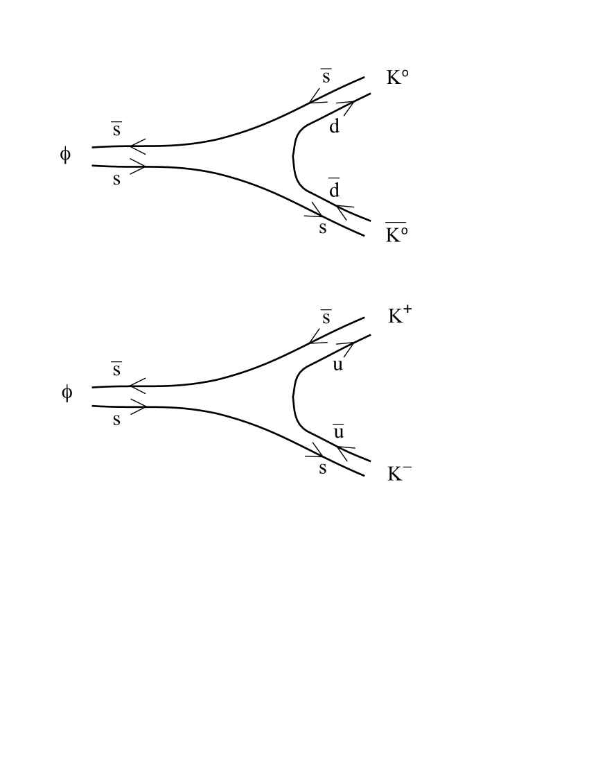
FIG. 1.: Quark model diagrams for $\phi\rightarrow K^{+}K^{-}$ and $\phi\rightarrow K^{0}\bar{K}^{0}$

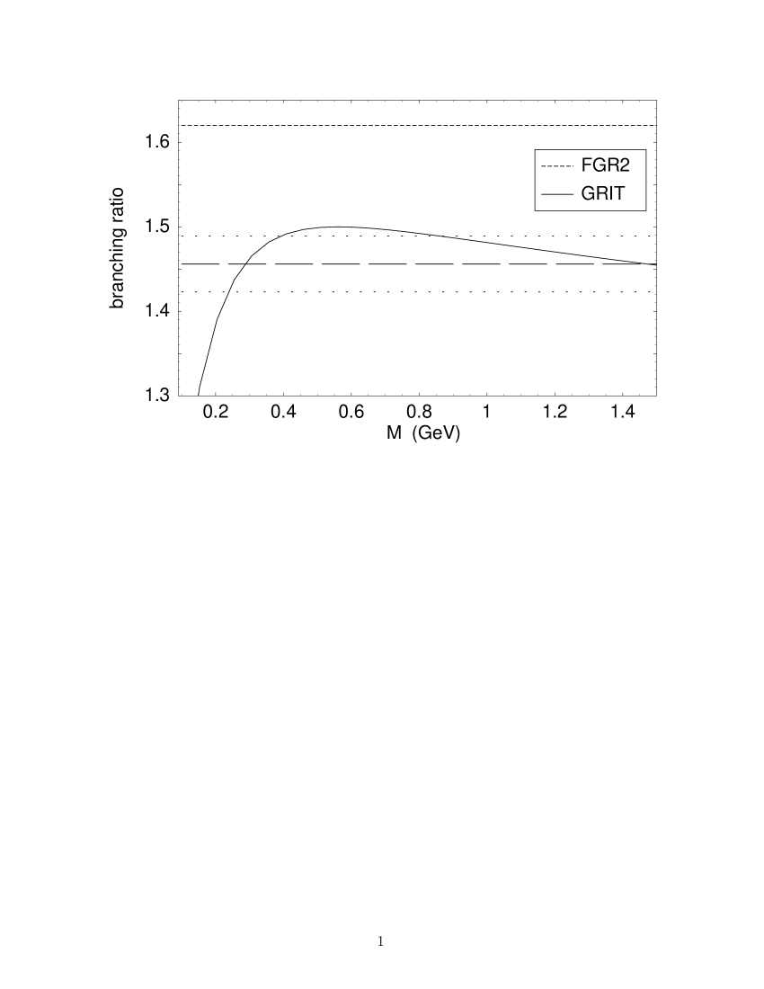
FIG. 2.: The solid curve gives the theoretical branching ratio versus $M$, the energy scale in Eq.(13), where $R_{th}=(g_{+}/g_{0})^{2}\eta R_{GRIT}\approx 1.063R_{GRIT}$. The experimental ratio in Eq.(10) is given by the long-dashed line, and the $1\sigma$ bounds fall within the dotted lines. The short-dashed line is the result predicted by FGR2.

FIG. 3.: The $K^{0}\bar{K}^{0}$ integrand in Eq.(11) multiplied by the square of the form factor, Eq.(13). For the central peak, the ordinate is obtained by adding 200 to the value shown.

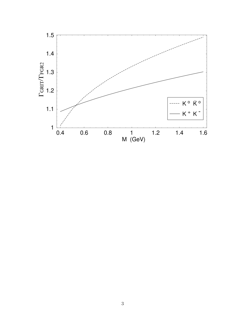
FIG. 4.: $\Gamma_{GRIT}/\Gamma_{FGR2}$ versus $M$ for both the $K^{+}K^{-}$ (solid curve) and $K^{0}\bar{K}^{0}$ (dashed curve) channels.