Oscillation induced neutrino asymmetry growth in the early Universe

Abstract:

We study the dynamics of active-sterile neutrino oscillations in the early universe using full momentum-dependent quantum-kinetic equations. These equations are too complicated to allow for an analytical treatment, and numerical solution is greatly complicated due to very pronounced and narrow structures in the momentum variable introduced by resonances. Here we introduce a novel dynamical discretization of the momentum variable which overcomes this problem. As a result we can follow the evolution of neutrino ensemble accurately well into the stable growing phase. Our results confirm the existence of a “chaotic region” of mixing parameters, for which the final sign of the asymmetry, and hence the SBBN prediction of ⁴He-abundance cannot be accurately determined.

1 Introduction

Recent observations from atmospheric and solar neutrinos from Super Kamiokande (SK)[1] and Sudbury Neutrino Observatory (SNO) [2] prefer conventional, mainly active-active mixings between ordinary electron, muon and tau neutrinos as the solutions to the observed flux deficits. However, while pure active-sterile solutions are disfavoured, sizable admixtures of sterile states in the observed fluxes are still allowed [3]. New sterile states are also needed in order to explain the LSND anomaly [4] by neutrino physics. Moreover, in a recent analysis of the so called “2+2”-models for four-neutrino mixing, the solutions with nonzero sterile neutrino components were found to provide best global fits to the solar, atmospheric and reactor data [6]. Corresponding limits on active-sterile mixings are quite generous, for example

$$\sin^{2}\theta_{\mu s} \lesssim 0.48 \qquad\rm(Atmospheric)$$

$$\sin^{2}\theta_{es} \lesssim 0.72 \qquad\rm(Solar\;\;LMA),$$ (1)

where LMA refers to the Large Mixing Angle solution for the solar neutrino deficit.

Active-sterile mixing, if realized, would have several interesting effects in astrophysical settings [7] and in particular for the evolution of the early universe [8, 9, 10, 11, 12, 14, 13, 15, 16, 17, 18, 19, 20]. In particular, sterile states could be brought into thermal equilibrium by mixing before nucleosynthesis, so that the resulting anomalous increase in the expansion rate of the universe would lead to overproduction of helium in disagreement with the observations [8, 9, 10, 11, 12, 13]. Excluding the parameter sets leading to equilibration provides useful bounds on active-sterile mixing. Indeed, from results of ref. [11] one can infer that the sterile components in mass eigenstates responsible for atmospheric anomaly and LMA are constrained by

$$\sin^{2}\theta_{\mu s} \lesssim 0.013 \qquad\rm(Atmospheric)$$

$$\sin^{2}\theta_{es} \lesssim 0.026 \qquad\rm(Solar\;\;LMA)$$ (2)

where we used a SBBN-limit of $N_{\nu}\lesssim 3.4$ for the number of effective neutrino degrees of freedom [11, 21]. These numbers correspond to the “light” case where the sterile component is the heavier of the mixing states; in the opposite, “dark” case, the corresponding limits are even stronger by one to two orders of magnitude. In either case the cosmological constraints are more stringent than those obtained in terrestrial laboratories.

While quite generic, the cosmological bounds (2) do depend on some simple prior assumptions, the most important of which is that the primordial lepton asymmetry is not anomalously large[14]. It may be possible to circumvent them in more complicated mixing schemes involving more sterile states (for a recent discussion, see [22]). In a particular attempt it was shown in ref. [15] that for a large negative $\delta m^{2}$ and a small enough mixing angle (so that the equilibration bounds of [11] can be avoided), say on the $\nu_{\tau}-\nu_{s^{\prime}}$-sector, resonant oscillations may trigger a rapid growth of the tau lepton asymmetry. This asymmetry could then become very large, $L_{\tau}\sim{\cal O}(1)$ and change the natural prior condition of no significant initial lepton asymmetry for a mixing in any other sectors. Indeed, if created early enough, such an asymmetry could suppress $\nu_{\mu}-\nu_{s}$-oscillations [23, 14], obviating the bounds (2) for $\nu_{\mu}-\nu_{s}$-mixing. However, as this scenario requires that the sterile state is the lighter one (resonance condition), and that the mass splitting $|\delta m^{2}|$ is large (to create $L_{\tau}$ early enough), it is essentially excluded by the recent solar and atmospheric neutrinos combined with the direct constraint on the electron neutrino mass [24].

Even with the mechanism of ref. [15] by and large excluded, there can be important effects due to $L$-growth with smaller $|\delta m^{2}|$. For example, a large homogeneous electron neutrino asymmetry $L_{\nu_{e}}$ would directly influence the nucleosynthesis prediction for the helium-4 abundance through the reactions

$$n+e^{+} \leftrightarrow p+\bar{\nu}_{e}$$

$$p+e^{-} \leftrightarrow n+\nu_{e}\;,$$ (3)

which keep the neutron-to-proton ratio in equilibrium at early times. Changing the electron neutrino abundance could tilt the balance of these reactions with the possibility of either increasing $Y_{He}$ (negative $L_{\nu_{e}}$), and hence strengthening the bounds (2), or decreasing $Y_{He}$ (positive $L_{\nu_{e}}$), leading to weakening of the bounds (2).

The physics involved with the resonant growth of the asymmetry is very complicated because of several vastly different physical scales both in the temporal direction and in momentum variable, which effect the evolution of the ensemble in an essential way. The relevant QKE’s are nonlinear and strongly coupled internally via the asymmetry term, and therefore no useful analytical approximation exists for the problem. Numerical solution is also greatly complicated by the various different physical scales, and while the phenomenon of asymmetry growth is fairly well established by now, the determinacy of the final sign of the asymmetry is still not well understood. The ambiguity was first observed in [16], and in [17, 19] it was shown that this “chaoticity” occurs in certain well defined region of mixing parameters. References [16, 17, 19] employed a numerical solution for the momentum averaged approximation of the QKE’s however, and their results were challenged by ref. [25], who claimed that the final asymmetry is always fully determined by the initial conditions. While the analysis of ref. [25] is now discredited [26], it still remains true that no numerically reliable momentum dependent analysis has so far shown the existence of the chaotic region. It is important to settle the issue because, as mentioned above, large $L_{\nu_{e}}$ could significantly alter the helium-4 abundance. Indeed, if the sign of $L_{\nu_{e}}$ were found to be chaotic, then $Y_{He}$ could not be reliably determined from BBN [17].

In this paper we study the dynamics of active-sterile neutrino oscillations in the early universe using full momentum-dependent quantum-kinetic equations (in homogeneous space). Our main technical improvement over the previous works is the introduction of a novel dynamical discretization method for the momentum variable which enables us to model accurately the density matrices over the entire momentum range, including the extremely pronounced and narrow structures close to resonant momenta. On physical context, our results confirm the existence of a ”chaotic” region of mixing parameters, for which the final sign of the asymmetry is not deterministic. It also confirms the expectation [17, 27], that the size of the chaotic region is somewhat smaller than indicated by the momentum averaged code [17]. These results can be seen as giving more strength on the cosmological constraints on neutrino mixing parameters.

The paper is organized as follows. In section 2 we set up the quantum kinetic equations for the problem. In section 3 we introduce the novel dynamically adjusted discretization of the momentum variable and in section 4 we set up our kinetic equations with this parametrization. The method we develop allows us to have enough resolution to solve the problem with relatively small number of momentum bins (we use at most 400 bins). In section 5 we display our numerical results for the key variables driving the oscillation and discuss the numerical stability of our solutions. Finally, in section 6 we present our results on the asymmetry growth and oscillations as well as the interpretation of the physical consequences, and the section 7 contains a summary and outlook.

2 Quantum Kinetic Equations

In the early Universe the oscillating neutrinos experience frequent scatterings which interrupt the coherent evolution of the state and introduce collisional mixing between different momentum states. The mathematical formalism which can incorporate all these features has been developed elsewhere [28, 10, 11, 29, 30], and it takes the form of the quantum kinetic equations for the reduced density matrices for the neutrino and antineutrino ensembles. We parametrize the density matrices by the Bloch vector presentation [11]:

$$\rho_{\nu}\equiv\frac{1}{2}f_{0}(P_{0}+{\bf P}\cdot{\bf\sigma})\;,\qquad\rho_{\bar{\nu}}\equiv\frac{1}{2}f_{0}(\bar{P}_{0}+{\bf\bar{P}}\cdot{\bf\sigma}),$$ (4)

where $\mathbf{\sigma}$ are the Pauli spin matrices and $f_{0}=(1+\exp(p/T))^{-1}$ is the Fermi-Dirac distribution function without chemical potential. Then to the the lowest order in the interaction [28, 10, 29, 30], the QKE’s for the density matrix take the form

$$d_{t}P_{0} = \phantom{-}\frac{\Gamma}{f_{0}}\left[f_{eq}-\rho_{\alpha\alpha}\right]$$

$$d_{t}P_{x} = -V_{z}P_{y}-DP_{x}$$

$$d_{t}P_{y} = \phantom{-}V_{z}P_{x}-V_{x}P_{z}-DP_{y}$$

$$d_{t}P_{z} = \phantom{-}V_{x}P_{y}+\frac{\Gamma}{f_{0}}\left[f_{eq}-\rho_{\alpha\alpha}\right]\,,$$ (5)

where $d_{t}\equiv\partial_{t}-Hp\partial_{p}$ and $H$ is the Hubble expansion factor. The rotation vector $\mathbf{V}$ has the following components ($V_{y}\equiv 0$): in $x$-direction one has only the vacuum contribution

$$V_{x}=\frac{\delta m^{2}}{2p}\sin 2\theta_{0}\;,$$ (6)

whereas in the $z$-direction also the matter induced effective potential contributes:

$$V_{z}=V_{0}+V_{1}+V_{L},$$ (7)

where

$$V_{0}\phantom{-} = -\frac{\delta m^{2}}{2p}\cos 2\theta_{0},$$ (8)

$$V_{1}^{e}\phantom{-} = -14\sqrt{2}\frac{\zeta(4)}{\zeta(3)}\frac{G_{F}}{M_{W}^{2}}N_{\gamma}p\;T\left(1+{\textstyle\frac{1}{4}}\cos^{2}\theta_{W}\left[n_{\nu_{e}}+n_{\bar{\nu}_{e}}\right]\right)$$ (9)

$$V_{1}^{\mu,\tau} = -\frac{7\sqrt{2}}{2}\frac{\zeta(4)}{\zeta(3)}\frac{G_{F}}{M_{Z}^{2}}N_{\gamma}p\;T\left[n_{\nu_{\mu,\tau}}+n_{\bar{\nu}_{\mu,\tau}}\right]$$ (10)

$$V_{L}\phantom{-} = \phantom{-}\sqrt{2}G_{F}N_{\gamma}L^{(\alpha)}.$$ (11)

Here $N_{\gamma}$ is the photon equilibrium number density, $n_{\nu_{\alpha,(\bar{\alpha})}}$ is the normalized to unity (in equilibrium) actual neutrino (antineutrino) number density, and the effective neutrino asymmetries $L^{(\alpha)}$ are given by

$$L^{(e)} = \left(\textstyle\frac{1}{2}+2\sin^{2}\theta_{W}\right)L_{e}+\left(\textstyle\frac{1}{2}-2\sin^{2}\theta_{W}\right)L_{p}-\textstyle\frac{1}{2}L_{n}+2L_{\nu_{e}}+L_{\nu_{\mu}}+L_{\nu_{\tau}}$$ (12)

$$L^{(\mu)} = L^{(e)}-L_{e}-L_{\nu_{e}}+L_{\nu_{\mu}}$$ (13)

$$L^{(\tau)} = L^{(e)}-L_{e}-L_{\nu_{e}}+L_{\nu_{\tau}}.$$ (14)

where $L_{f}\equiv(n_{f}-n_{\bar{f}})N_{f}/N_{\gamma}$.

The repopulation term $\Gamma(f_{eq}-\rho_{\alpha\alpha})$ in the diagonal part of (5) is written in the relaxation time approximation [31]. The distribution $f_{eq}$ in the repopulation term is the usual equilibrium Fermi-Dirac distribution

$$f_{eq}=\frac{1}{1+e^{\frac{p}{T}-\frac{\mu}{T}}}.$$ (15)

and the reaction rates are

$$\Gamma=C_{\alpha}G_{F}^{2}pT^{4}$$ (16)

with $C_{e}\simeq 1.27$ and $C_{\mu,\tau}\simeq 0.92$[11]. The damping terms $DP_{i}$ correspond to the decohering scatterings, which tend to destroy the coherence of the oscillation. In density matrix language such terms appear as relaxation terms suppressing the off-diagonals of the density matrix, or equivalently the $P_{x,y}$-components of the Bloch vectors. The magnitude of the decohering terms is just half of the corresponding scattering rate

$$D=\frac{1}{2}\Gamma.$$ (17)

The equation of motion for anti-neutrinos can be found by substituting $L^{(\alpha)}=-L^{(\alpha)}$ and $\mu_{\nu}=-\mu_{\nu}$ to the above equations (the latter condition is true when neutrinos are in chemical equilibrium).

The repopulation term used above is only an approximation for the correct elastic collision integral, and unfortunately it breaks the lepton number conservation. This is not a serious problem however, and it can be circumvented by introducing an explicit lepton number conserving evolution equation for $L^{(\alpha)}$. The appropriate equation, introduced in [27], is

$$d_{t}L^{(\alpha)}=\frac{1}{8\zeta(3)}\int\limits_{0}^{\infty}dp\;p^{2}(V_{x}P_{y}-\bar{V}_{x}\bar{P}_{y}).$$ (18)

Equation (18) can be derived from the original equations in the approximation where the $L$-violation due to the the approximate repopulation term is neglected. So, when using (18) to evolve $L$, it is guaranteed that the repopulation term does not directly affect the lepton asymmetry generation. The accuracy of the method can be monitored by comparing the value of $L^{(\alpha)}$ derived from (18) and from directly integrating the neutrino distribution functions. In practice the agreement was always to be good.

Neutrino and antineutrino sectors are extremely strongly coupled through the asymmetry $L^{(\alpha)}$ in equations (5). In order to compute $L^{(\alpha)}$ accurately enough despite the numerical round-off errors, it is then necessary to avoid computing $L^{(\alpha)}$ through differences of large quantities, such as naively appear in the equation (18). To this end we will define the “small” and “large” linear combinations of dynamical variables in particle and antiparticle sector

$$P_{i}^{\pm}=P_{i}\pm\bar{P}_{i}.$$ (19)

For convenience we also separate active and sterile sectors by defining

$$P_{a}^{\pm} =P_{0}^{\pm}+P_{z}^{\pm} =2\rho_{\alpha\alpha}^{\pm}/f_{0}$$ (20)

$$P_{s}^{\pm} =P_{0}^{\pm}-P_{z}^{\pm} =2\rho_{ss}^{\pm}/f_{0}.$$ (21)

In terms of variables (20-21) the equations take the form

$$d_{t}P_{a}^{\pm} = \phantom{-}V_{x}P_{y}^{\pm}+\Gamma\left[2f_{eq}^{\pm}/f_{0}-P_{a}^{\pm}\right],$$ (22)

$$d_{t}P_{s}^{\pm} = -V_{x}P_{y}^{\pm},$$ (23)

$$d_{t}P_{x}^{\pm} = -(V_{0}+V_{1})P_{y}^{\pm}-V_{L}P_{y}^{\mp}-DP_{x}^{\pm},$$ (24)

$$d_{t}P_{y}^{\pm} = \phantom{-}(V_{0}+V_{1})P_{x}^{\pm}+V_{L}P_{x}^{\mp}-\frac{1}{2}V_{x}(P_{a}^{\pm}-P_{s}^{\pm})-DP_{y}^{\pm},$$ (25)

where we assumed $\Gamma=\bar{\Gamma}$ and defined

$$f_{eq}^{\pm}=f_{eq}(p,\mu)\pm f_{eq}(p,-\mu)$$ (26)

Because $\bar{V}_{x}=V_{x}$, the equation for the asymmetry now reads simply

$$d_{t}L^{(\alpha)}=\frac{1}{8\zeta(3)}\int\limits_{0}^{\infty}dp\;p^{2}V_{x}P_{y}^{-}.$$ (27)

Finally, due to the particular form of the differential operator $d_{t}=\partial_{t}-Hp\partial_{p}$, it is possible to reduce our set of partial differential equations to ordinary differential equations by changing variables $p\rightarrow x\equiv p/T$, and $t\rightarrow T$, and correspondingly using the time-temperature relation

$$\frac{dT}{dt}=-HT.$$ (28)

The differential operator then becomes simply

$$d_{t}\rightarrow-\frac{1}{HT}\partial_{T}.$$ (29)

Let us stress that our introducing the small and large linear combinations is an absolutely necessary step for obtaining reliable solutions to QKE’s (22-25,27). This can best be appreciated from the figure (3) below, where we show the energy spectrum in neutrino and antineutrino sectors for a representative set of oscillation parameters; the asymmetry corresponds to the integral over the difference (not even visible!) of the neutrino and antineutrino distributions displayed.

3 Discretization of the momentum variable

While necessary, introducing parametrization (19) is unfortunately not sufficient to tackle the momentum dependent QKE’s. Additional difficulties arise due to structures in the momentum direction (in variable $x$) and in particular the very narrow ones introduced by the resonances. In this paragraph we explain step by step how we discretize the momentum variable such that these difficulties can be overcome.

First, the momentum variable ranges over the semi-infinite range $x\in[0,\infty]$, but in practice we will introduce cut-offs to both ends of spectrum. First, the ultra-relativistic neutrino approximation breaks down when $x\rightarrow 0$, formally appearing as a singularity in at $x=0$ in our equations. Second, it is useful to cut out very large $x$, in the exponentially suppressed tail of the distribution. So, we restrict $x$ to a range $x\in[x_{min},x_{max}]$, where in practice it suffices to use $x_{min}=10^{-4}$ and $x_{max}=100$.

Second, the variable $x$ is not ideal for discretization, because most of the variation in the spectrum occurs at small $x\lesssim 3$. We therefore have mapped the variable $x$ to $u(x)$ belonging to range $[0,1]$ by a transformation

$$u(x)=\frac{x(1+\epsilon_{2})-x_{\rm ext}\epsilon_{1}}{x+x_{\rm ext}}.$$ (30)

where $\epsilon_{1}\equiv k_{1}(1+\epsilon_{2})$ and $\epsilon_{2}\equiv(1+k_{1})/(k_{2}-k_{1})$ with $k_{1}\equiv x_{\rm min}/x_{\rm ext}$ and $k_{2}\equiv x_{\rm max}/x_{\rm ext}$. Apart from a small correction due to the cut-off parameters (30) is designed so that the extremum point of the thermal momentum distribution $x_{ext}$ gets mapped to $u\simeq 1/2$. We will also need the inverse of this function, which is

$$x(u)=\frac{x_{\rm ext}(u+\epsilon_{1})}{1+\epsilon_{2}-u}.$$ (31)

While clearly a significant improvement for binning the momentum variable, (30) is not clever enough to solve the numerical problems arising from the the pronounced structures around the resonant momenta. Fortunately, the resonance positions $x_{r_{1}}$ and $x_{r_{2}}$ can be solved analytically from the conditions $V_{z}=0$ (neutrinos) and $\bar{V}_{z}=0$ (antineutrinos):

$$x_{r_{1}} = \sqrt{\varphi^{2}+\chi}-\varphi\qquad\bar{\nu}{\rm-resonance}$$ (32)

$$x_{r_{2}} = \sqrt{\varphi^{2}+\chi}+\varphi\qquad\nu{\rm-resonance}$$ (33)

where in the case of $\nu_{\mu}$ and $\nu_{\tau}$ neutrinos

$$\varphi = \frac{\zeta(3)M_{Z}^{2}L^{(\alpha)}}{14\zeta(4)T^{2}}\approx 6.60\times 10^{8}L^{(\alpha)}T^{-2}_{\mathrm{\;MeV}}$$ (34)

$$\chi = \frac{\zeta(3)M_{Z}^{2}|\delta m^{2}|\cos 2\theta_{0}}{14\sqrt{2}\zeta(4)G_{F}N_{\gamma}T^{3}}\approx 1.64\times 10^{8}|\delta m^{2}|_{\mathrm{\;eV}^{2}}\cos 2\theta_{0}T^{-6}_{\mathrm{\;MeV}}.$$ (35)

Using (30) one easily finds the corresponding resonant values in the $u$-variable.

The resonance widths can be estimated from the distance over which the matter mixing angle drops to a some fraction of its maximum value of unity. In this way one finds that the relative resonance width is proportional to the vacuum mixing angle:

$$\frac{\Delta x}{x}\sim\tan 2\theta_{0}.$$ (36)

From (36) it is clear that for small mixing angles the structures near resonances can only be resolved by an extremely finely spaced momentum grid. For example with $\sin^{2}2\theta_{0}=10^{-6}$, equation (36) predicts structures in the scale $\Delta x/x\simeq 10^{-3}$. Assuming then that at least 50 points are needed to describe the resonant region accurately, one sees that a linear binning of the $x$-variable with $x_{max}=100$ would require $5\times 10^{6}$ grid points! Solving such problem is clearly beyond capabilities of any computer we have today.

Our mapping (30) helps the situation by roughly a factor of hundred, but the remaining problem would still be way too large. We therefore need to find a second transformation $u\rightarrow u(v)$ that would redistribute the points such that more grid points are clustered around the resonances in the physical momentum variable. There are obviously many ways to implement such a transformation. We found it most convenient to construct it by using polynomials of the form $a+b(v-v_{r})^{3}$. Because we have two resonance points the mapping function is a little complicated:

$$u(v)=\alpha v+(a+b(v-v_{r_{1}})^{3})\,\theta(v_{c}-v)+(c+d(v-v_{r_{2}})^{3})\,\theta(v-v_{c}),$$ (37)

where the two separate mappings around resonant values $v_{r_{1}}$ and $v_{r_{2}}$ are joined smoothly at the geometric mean of the resonances $v_{c}\equiv\frac{1}{2}(v_{r_{1}}+v_{r_{2}})$. The linear term $\alpha v$ was added in order to have a control how steep is the distribution function of the grid points.

The mapping (37) has six free parameters $a$, $b$, $c$, $d$, $v_{r_{1}}$ and $v_{r_{2}}$, which will be determined from boundary conditions at $v=0$ and $v=1$ and continuity conditions at $v=v_{c}$. First, the constants $a$, $b$, $c$ and $d$ are fixed by the boundary conditions

$$u(0) = 0,$$ (38)

$$u(v_{r_{1}}) = u_{r_{1}},$$ (39)

$$u(v_{r_{2}}) = u_{r_{2}},$$ (40)

$$u(1) = 1,$$ (41)

which results in

$$a = u_{r_{1}}-\alpha v_{r_{1}}$$ (42)

$$b = \frac{u_{r_{1}}}{v_{r_{1}}^{3}}-\frac{\alpha}{v_{r_{1}}^{2}}$$ (43)

$$c = u_{r_{2}}-\alpha v_{r_{2}}$$ (44)

$$d = \frac{1-u_{r_{2}}}{(1-v_{r_{2}})^{3}}-\frac{\alpha}{(1-v_{r_{2}})^{2}}.$$ (45)

Note that $u_{r_{i}}$ are not unknowns, but can be solved analytically from the resonance conditions (32-33) and the inverse mapping (31). Finally, the continuity conditions

$$\lim_{v\rightarrow v_{c}+} u(v) =\lim_{v\rightarrow v_{c}-}u(v)$$ (46)

$$\lim_{v\rightarrow v_{c}+} \partial_{v}u(v) =\lim_{v\rightarrow v_{c}-}\partial_{v}u(v).$$ (47)

provide implicit equations for the remaining two unknowns $v_{r_{i}}$:

$$a+\frac{1}{8}b(v_{r_{2}}-v_{r_{1}})^{3} = c+\frac{1}{8}d(v_{r_{1}}-v_{r_{2}})^{3}$$ (48)

$$b = d.$$ (49)

Unfortunately these are sixth order algebraic equations and can only be solved by iterative numerical algorithms.

Figure 1: The mapping $u=u(v)$ is shown with $L^{(\alpha)}=4\times 10^{-7}$, $T=11\mathrm{\;MeV}$ (solid line) and with $L^{(\alpha)}=10^{-10}$, $T=15\mathrm{\;MeV}$ (dashed line). Mixing parameters are $\delta m^{2}=-0.1\mathrm{\;eV}^{2}$ and $\sin^{2}2\theta_{0}=10^{-9}$.

Figure 2: Density of points (defined as the inverse of the step size) in the physical momentum variable $x$ for the transforms shown in figure (1).

The novel feature of the above change of variables is that it automatically follows the resonances, placing majority of the grid points dynamically in their vicinity. As an alternative to our approach, one could think of using library routines with automatic grids to take care of this distribution. However, the resonance positions evolve as a function of expansion scale of the universe and in particular as a function of $L^{(\alpha)}$. High point densities are thus needed at different momenta at different times, and this movement can be fast. None of the library routines we tried came close to being able to cope with these requirements and failed completely to solve the problem. With our parametrization on the other hand, the numerical program can be written for a fixed grid in the variable $v$, and the redistribution of points is provided by the dynamical equations themselves.

In Fig. (1) we show the transformations $u\rightarrow v$ when $L^{(\alpha)}$ is almost zero (dotted line), and when $L^{(\alpha)}$ has grown to a substantial value (solid line). In the former case one cannot distinguish the two resonances by eye, whereas in the second case the structures have become very distinct. Fig. (2) shows the density of points as a function of $x$ (defined as the inverse of separation of grid points in the $x$-variable).

4 Changes in the QKE’s due to the parametrization

The changes of variables (30) and (37) affect the partial derivatives appearing in Eqns. (22-25,27). These equations have been written assuming the evolution of $\rho$ and $L$ is along constant $x$ contours. However, we have now fixed our grid in the variable $v$, and hence need to find the evolution equations with $T$ and $v$ as the independent variables. These are easily found from the old ones by the chain rule partial differentiation

$$\Big{(}\frac{\partial\rho\left(T,x(T,v)\right)}{\partial T}\Big{)}_{v} = \Big{(}\frac{\partial\rho}{\partial T}\Big{)}_{x}+\Big{(}\frac{\partial x}{\partial T}\Big{)}_{v}\,\Big{(}\frac{\partial\rho}{\partial x}\Big{)}_{T}$$ (50)

$$= \Big{(}\frac{\partial\rho}{\partial T}\Big{)}_{x}+\Big{(}\frac{\partial x}{\partial T}\Big{)}_{v}\Big{(}\frac{\partial u}{\partial x}\Big{)}_{T}\Big{(}\frac{\partial v}{\partial u}\Big{)}_{T}\,\Big{(}\frac{\partial\rho}{\partial v}\Big{)}_{T}$$

$$= \Big{(}\frac{\partial\rho}{\partial T}\Big{)}_{x}+\Big{(}\frac{\partial u}{\partial T}\Big{)}_{v}\Big{(}\frac{\partial v}{\partial u}\Big{)}_{T}\,\Big{(}\frac{\partial\rho}{\partial v}\Big{)}_{T}\,.$$

In the last equality we used the fact that $u=u(x)$ only. The differentials $(\partial_{T}\rho)_{x}$ are of course just given by the l.h.s. of equations (25), and the last coefficient $(\partial_{v}\rho)_{T}$ is computed numerically as a part of the system of the partial differential equations. To be precise, we are using the central derivative formula

$$\left(\frac{\partial\rho}{\partial v}\right)_{T}=\frac{\rho(v+h)-\rho(v-h)}{2h}.$$ (51)

Of the remaining differentials $(\partial_{v}u)_{T}$ is also easily solved from the parametrization Eq. (37:

$$\left(\partial_{v}u\right)_{T}=\frac{1}{\alpha+3[b(v-v_{r_{1}})^{2}\,\theta(v_{c}-v)+d(v-v_{r_{2}})^{2}\,\theta(v-v_{c})]}.$$ (52)

However, solving the remaining differential $\left(\partial_{T}u\right)_{v}$ is somewhat more complicated. Using equation (37) one can write

$$\left(\partial_{T}u\right)_{v} = \phantom{-}\left[\partial_{T}a+\partial_{T}b(v-v_{r_{1}})^{3}-3b(v-v_{r_{1}})^{2}\partial_{T}v_{r_{1}}\right]\theta(v_{c}-v)$$ (53)

$$+\left[\partial_{T}c+\partial_{T}d(v-v_{r_{2}})^{3}-3d(v-v_{r_{2}})^{2}\partial_{T}v_{r_{2}}\right]\theta(v-v_{c}),$$

where

$$\partial_{T}a = \partial_{T}u_{r_{1}}-\alpha\partial_{T}v_{r_{1}}$$ (54)

$$\partial_{T}b = \frac{1}{v_{r_{1}}^{3}}\left(\partial_{T}u_{r_{1}}+\Big{(}2\alpha-\frac{3u_{r_{1}}}{v_{r_{1}}}\Big{)}\partial_{T}v_{r_{1}}\right)$$ (55)

$$\partial_{T}c = \partial_{T}u_{r_{2}}-\alpha\partial_{T}v_{r_{2}}$$ (56)

$$\partial_{T}d = -\frac{1}{(1-v_{r_{2}})^{3}}\left(\partial_{T}u_{r_{2}}+\Big{(}2\alpha-3\frac{1-u_{r_{2}}}{1-v_{r_{2}}}\Big{)}\partial_{T}v_{r_{2}}\right).$$ (57)

Here the only unknowns are the temperature derivatives of the resonances in the $v$-variable $\partial_{T}v_{r_{i}}$. These can be solved from our original matching conditions (48) and (49), which can formally be written as

$$f_{1}\left(v_{r_{1}}(T),v_{r_{2}}(T),T\right) = 0$$ (58)

$$f_{2}\left(v_{r_{1}}(T),v_{r_{2}}(T),T\right) = 0.$$ (59)

Differentiating equations (58-59) with respect to $T$ results in a linear set of equations for $\partial_{T}v_{r_{i}}$, which after a little algebra can be brought to the form

$$\partial_{T}v_{r_{i}}=U_{ij}\partial_{T}u_{r_{j}},$$ (60)

where the matrix $U_{ij}$ depends both on $u_{r_{i}}$ and $v_{r_{i}}$. Note that despite the apparent complexity of our parametrization, we have been able to reduce everything except solving for the resonance parameters $v_{r_{i}}$ to a simple linear algebra. Solving $v_{r_{i}}$ from the matching equations at each time step would be very time consuming however. This is so in particular because we need to solve them with very high accuracy in order for not to lose the continuity of the matching at $v=v_{c}$ and to avoid inducing random numerical errors into the equations. Fortunately, the equation (60) itself offers the way out of this problem. Namely, we only need to solve $v_{r_{i}}$ from the matching conditions (48) and (49) once, in the beginning of the iteration, as their value can later be evolved by equations (60) as the solution proceeds. In this way even solving for the parametrization from $v$ to $x$ becomes part of the dynamical equations. The accumulation of numerical error can be easily traced by solving the matching conditions independently for some temperatures. In practice the errors do not accumulate at all and it turns out that using the differential equation is by far the superior method for solving $v_{r_{i}}$ in comparison to using the matching conditions at each temperature step.

5 Numerical Results

We have solved the evolution equations numerically for a range of representative parameter sets. In figure (3) we show the neutrino and antineutrino distribution functions in a relatively early stage in the evolution for $\delta m^{2}=-10\;\rm eV^{2}$ and $\sin^{2}2\theta_{0}=10^{-6.1}$. The distributions show a very nice thermal shape, and no visible difference between particle and antiparticle sectors can be seen. This is so despite the fact that at the temperature at which the distributions were plotted, the momenta $p\simeq 1.8T$ are currently resonant (indicated by the gray line in the plot); the amplitude of resonant structure is simply too small to be seen in the scale of the “large variables”.

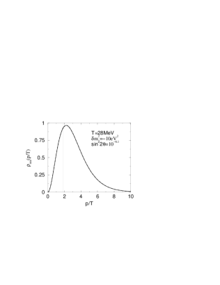
Figure 3: Example of neutrino ($\rho_{\alpha\alpha}$) and antineutrino ($\rho_{\bar{\alpha}\bar{\alpha}}$) spectra as a function of $p/T$. Lines fall on top of each others. Gray line marks the resonance momenta.

The resonance does alter the asymmetry spectrum however. In figure (4) we show the distribution of the difference of neutrino and antineutrino densities $\rho_{\alpha\alpha}-\rho_{\bar{\alpha}\bar{\alpha}}$ in the physical variable $x$. The prominent and extremely narrow resonance structure (one cannot separate the neutrino and antineutrino resonances here) is clearly visible. The same spectrum is shown in the integration variable $v$ in figure (5). Now the sharp kink-like resonant structure has broadened into a broad wave, which is easily represented by the linearly discretized function in variable $v$ (grid points are shown by the open circles). In this example we used just 400 grid points, but essentially identical results were found with only 200 points. Moreover, comparing the scales in figures (3-4), one sees that the scale of variation of $L(x)$ is ten orders of magnitude below unity. So, in order to follow the evolution of $L^{(\alpha)}$ accurately when using the original variables, one should be able to integrate over distributions with an accuracy much better than ten digits! This seems totally impossible, and clearly indicates that our use of variables $P^{\pm}$ is essential.

Figure 4: Difference of neutrino and antineutrino densities $\rho_{\alpha\alpha}-\rho_{\bar{\alpha}\bar{\alpha}}$ as a function of $p/T$ for the same parameters as in figure 3.

Figure 5: Same as figure (4), but shown against variable $v$.

These examples prove the success of the key elements in our approach, namely that by separating the small and large variables, and by introducing the novel dynamical discretization of the momentum grid, we can model the evolution of the ensemble of oscillating neutrinos accurately. Moreover, we can do so using small enough lattices such that the code can be run even in a powerful modern workstation (although a single run may then take as long as a couple of days).

5.1 Regulating the sterile neutrino spectrum

As one lets the system evolve further the resonance $x$ moves to larger values while the integrated $L^{(\alpha)}$ decreases. This continues until one reaches roughly the point when the main bulk of the active neutrino distribution is getting through the resonance. At this point one expects that the total asymmetry begins to oscillate or grow, depending on the parameters. In our initial runs we did not get that far however, but the program crashed due to an accumulation of structures in sterile neutrino spectrum with momenta less than $x_{res}T$. How these structures arise is easy to understand. Indeed, the active sector distributions are kept smooth away from the resonances by diffusion induced by collisions with the background particles. Sterile states interact only through the effective interaction due to mixing however, and since this interaction is neglibly small away from the resonances, the diffusion does not work on sterile sector. As a result the moving resonance leaves the sterile neutrino momentum distribution quite oscillatory for $x<x_{res}$. While these developments in the sterile sector have little effect on variables in the active sector (because active and sterile states are essentially decoupled away from resonances), they still pose a numerical problem: as the resonance moves forward in $x$, the density of points reduces drastically in the region $x\ll x_{res}$, until the point that the grid becomes too sparse to model the oscillatory structures in the unsmoothed sterile neutrino distribution. Eventually the amplitudes of these structures overflow causing numerical instability and the solution breaks down.

The above explanation of the instability also suggests an obvious cure for the problem. If one is not interested in studying the sterile neutrino asymmetry spectrum, all we need to do is to add a small regulatory interaction term to sterile neutrino sector, which will smooth their distribution away from resonances, and yet does not alter the evolution of the variables in the active sector. The latter requirement can be met by a suitable form of the interaction term and by making it small enough so that it does not change the physics in the resonance region. The challenge is to do this so that the regulatory term remains efficient enough to numerically stabilize the system. To this end we have added the following “sterile repopulation terms” onto equation (23):

$$R_{\nu_{s}}^{+} = r_{s}\Gamma\left(n_{\nu_{s}}f_{eq}^{+}(x,\mu)-\rho_{ss}^{+}\right)$$ (61)

$$R_{\nu_{s}}^{-} = r_{s}\Gamma\left(\rho_{aa}^{\rm init}-\rho_{aa}^{-}-\rho_{ss}^{-}\right).$$ (62)

Here $\rho_{aa}^{\rm init}$ is the initial density matrix in the active sector. We used the active sector interaction rate $\Gamma$ above, and let the parameter $r_{s}$ control the size of the regulatory term. The regulators (61-62) differ from the repopulation terms in the active sector in (22) in that we have added normalization factors to make sure that the integrals over $R_{\nu_{s}}^{\pm}$ always vanish. (In this way we avoid spurious sterile state equilibration even with large control parameter $r_{s}$.)

We obviously need to show that there exists a range of values for which the results converge and become independent of $r_{s}$, while the regulator still continues to stabilize the solution. That we do reach this goal is evidenced in Fig. (6), where we show the evolution of the total asymmetry for $r_{s}=0.1$, 0.01, 0.001, $10^{-4}$ and $10^{-5}$, for $\delta m^{2}=-0.1\mathrm{\;eV}^{2}$ and $\sin^{2}2\theta_{0}=10^{-6.1}$. Unsurprisingly, for large $r_{s}$ there is a significant effect, but for small $r_{s}$ the results do converge to the point that no visible difference can be seen between the two curves corresponding to two smallest $r_{s}$’s. Let us stress that the mixing parameters were here deliberately chosen such as to show a particularly large sensitivity for the regulator. For many other cases that we studied it would have been difficult to show any effect at all; for example the results displayed in figure (8) showed no appreciable dependence on the regulator up to $r_{s}=10$.

Figure 6: The stability of asymmetry evolution against variation of parameter $r_{s}$. We have used values $r_{s}=0.0001$ (solid line), 0.001 (dashed line), 0.01 (dotted line) and 0.1 (dash-dotted line). Solutions for values $r_{s}=10^{-4}$ and $r_{s}=10^{-5}$ (long dashed line) are already indistinguishable in the figure. Oscillation parameters are $\delta m^{2}=-0.1\mathrm{\;eV}^{2}$ and $\sin^{2}2\theta_{0}=10^{-6.1}$.

We have also studied the stability of our results against changes in various numerical error handling parameters in our code. The stepwise error tolerance for example can be relaxed by an order of magnitude from what we actually employed, before any visible deviation from the solution can be seen over the entire integration range. This is true also for our examples corresponding to the oscillatory solutions in or near the chaotic region. Of course, the numerical accuracy would be eventually compromised for parameters for which the asymmetry undergoes very large number of oscillations before settling to the growing curve, but as in [17], that does not affect our main conclusions. Also cut off parameters $x_{min}$ and $x_{max}$ and the tilt $\alpha$ which controls the density of points at the resonance can be varied within reasonable limits without any observable effects on the results. We therefore are confident that our observed pattern of asymmetry oscillations is indeed physical, and not of numerical origin.

5.2 Argument for chaoticity in $L$-growth

Having introduced a method that can handle the evolution of momentum dependent density matrices and in particular the asymmetry, and having proven its numerical stability and accuracy, we now pursue the question of the “chaotic” behaviour of the final sign of the integrated asymmetry. Note that while the use of word chaos is customary in this context, we strictly speaking mean only sensitivity of the final sign of the asymmetry on initial seed asymmetry and on oscillation parameters.

In the context of our earlier work using the momentum averaged equations [17, 19], we explained what was the physical origin for the sign sensitivity. Quite simply, changes in the boundary conditions (initial baryon asymmetry and the oscillation parameters) change the direction of the motion of the system, and the topography of the attractor solutions in the phase space at the onset of resonance. Roughly speaking, in the momentum averaged case one can draw an analogy between the system and a somewhat sticky ball initially rolling down a single valley floor that later branches to two, with a low maximum in between, at the resonance point. Changing baryon asymmetry would then be analogous to changing the speed and direction of the ball at the branching point and changing oscillation parameters to that of changing the shape of the valleys themselves. Sign sensitivity arises for those initial conditions and valley forms for which the ball makes many oscillations between the two degenerate valleys before stickiness (damping) eventually wins and makes it to settle into either one of them.

In the momentum dependent case these structures become smeared out, and to draw a mechanical analogy, one should rather think, instead of a ball, of a string of varying size beads (largest ones in the middle, corresponding to the peak in the thermal distribution) coupled by a very elastic cord, wiggling down the valleys described above. While this is obviously a much more complicated system with qualitatively new features, one would still expect to see oscillations in the weighted average position of beads at least when the largest ones roll past the branching point (in $L$ when the maximum of the distribution crosses the resonance). Moreover, if the average position of the string ($L$) makes many oscillations over the central hill before stickiness (damping) wins, one again should expect that the final valley that the string settles in (sign of $L$) strongly depends on initial and boundary conditions. While this analog is certainly bears only a crude resemblance to the true system, it should help convince the reader of the fact that there is nothing mysterious about the sign sensitivity in the $L$-evolution, but that it is rather something to be expected.

Obviously, all we need to do to prove the existence of chaoticity, is to find examples of almost identical sets of oscillation parameters for which the final asymmetry does show significantly different oscillation pattern, and leads to a different final sign. We show such a case in figure (7). All three curves in the figure correspond to $\delta m^{2}=-10\mathrm{\;eV}^{2}$ but have slightly different vacuum mixing angles. The two curves which behave almost alike, have mixing angles $\sin^{2}2\theta_{0}=10^{-6.1}$ (solid curve) and $\sin^{2}2\theta_{0}=10^{-6.099}$ (dotted curve) respectively. The dash-dotted curve with a very different behaviour corresponds to $\sin^{2}2\theta_{0}=10^{-6.09}$. So, if such mixing were ever observed and the mixing angle was measured to a precision better than a tenth of a per cent, the final sign of the lepton asymmetry and its effect on nucleosynthesis could be predicted from our computation. However, if the mixing angle was measured with less than about one per cent accuracy, we would not be able to say what the final asymmetry will be, and therefore what is the precise BBN prediction for helium abundance.

Figure 7: Neutrino asymmetry oscillations are shown near the boundary of ”chaotic” region using same $\delta m^{2}=-10\mathrm{\;eV}^{2}$ and three slightly different mixing angles $\sin^{2}2\theta_{0}=10^{-6.1}$ (solid line) $\sin^{2}2\theta_{0}=10^{-6.099}$ (dotted line) and $\sin^{2}2\theta_{0}=10^{-6.09}$ (dash-dotted line).

The sign sensitivity does not occur for all oscillation parameters, however. In the figure (8) we show results from “stable” region of parameters (same mass difference as above, but much smaller mixing angle). In this case, while visible differences in the evolution become visible when mixing angle is changed by a factor or three, the asymmetry never becomes oscillatory, and the final sign is determined by the initial sign of the asymmetry.

Figure 8: Asymmetry evolution in the stable region of oscillation parameters. All curves corresponds to mass splitting $\delta m^{2}=-0.1\;\rm eV^{2}$ and the mixing angles are $\sin^{2}2\theta_{0}=10^{-9}$ (solid curve), $\sin^{2}2\theta_{0}=10^{-8.9}$ (dotted curve) and $\sin^{2}2\theta_{0}=10^{-8.5}$ (dashed curve).

Our first example was chosen from close to the edge of the chaotic region, and just as making $\sin^{2}2\theta_{0}$ smaller made system more stable, increasing it has the opposite effect. The number of oscillations and also degree of sensitivity of the final sign to the oscillation parameters increases very rapidly with $\sin^{2}2\theta_{0}$. Nevertheless, the degree of sensitivity to parameters is weaker and thus the chaotic region smaller than what was found in the momentum averaged treatment [17]. Quantitatively our new results agree roughly with the boundaries of the chaotic region inferred in [27], but since the numerical work is, even with the improvements we have made, very time consuming, we will not attempt a precise mapping of the chaotic region here.

Let us finally to try to understand a little more deeply what precisely drives the oscillations of the total asymmetry in the momentum dependent case. A clue can be found from Figure (9) which shows the variable $P_{y}^{-}$ in the region where the asymmetry oscillates significantly. (At earlier times, when the total $L$ does not oscillate, the structure of the $P_{y}^{-}$-spectrum is similar to that of $\rho_{\alpha\alpha}^{-}$ shown in Fig. (5).) The two new peaks seen outside the resonance grow slowly in time, while their sign oscillates rapidly. Because these structures are asymmetric around the resonance (in the physical variable $x$), the integral over $P_{y}^{\pm}(x)$ is nonzero and oscillates. As a result also $L$, which is solved from (27), becomes oscillatory.

What causes these structures, is a delicate interplay between the coherence length and the matter oscillation length. The former is simply given by the inverse of the damping rate $\ell_{\rm coh}=1/D$ and the latter is

$$\ell_{\rm m}=\frac{l_{\rm vac}}{\sqrt{1-2\chi\cos 2\theta_{0}+\chi^{2}}}$$ (63)

where $l_{\rm vac}\equiv 4\pi p/|\delta m^{2}|$ and $\chi\equiv 2p|V|/|\delta m^{2}|$ where $|V|$ is the magnitude of the matter contribution to the $V_{z}$ in equation (7). Near the resonance the matter oscillation length is very long, and in particular at high temperatures it exceeds the coherence length by a large margin. In such a situation the resonance is strongly overdamped, and despite the maximal mixing angle oscillations do not have time to develop because the state is continuously projected to the active direction. This in part explains why the resonant features have so modest amplitudes at early times (cf. Fig. (4)).

Figure 9: Lower panel: Variable $P_{y}^{-}$ as a function of $v$ at temperature $T=27.8\mathrm{\;MeV}$ for oscillation parameters $\delta m^{2}=-10\mathrm{\;eV}^{2}$, $\sin^{2}2\theta_{0}=10^{-6.099}$. Upper panel: The coherence length (dashed line) and $l_{\rm m}/4$ (solid line) for the same parameters. Physical momentum at the resonance is $x_{\rm res}=1.88$.

In the upper panel of the figure (9) we have plotted the coherence length and $\ell_{\rm m}/4$, which corresponds to the distance over which $P_{y}^{\pm}$ first rises to maximum due to oscillation. It is clear that the new structures correspond to the case when the matter oscillations first time break the overdamping situation. Further away from the resonance the damping no more can block the oscillations, but since the matter mixing angle decreases very fast away from the resonance, the amplitude of the oscillation features dies off quickly. As the temperature decreases, the new structures move away from the resonance, and they also become broader (one can show that their separation scales like $\delta x\sim T^{-3}$). This is why their amplitude slowly increases in time (with decreasing $T$) causing larger and larger amplitude oscillations in the total asymmetry $L$. The lesson to bring home from these observations is that the dynamics of $L$-growth and oscillations is very dependent on the detailed fine structure of the various components of the density matrix. Such fine details on the hand can only be studied in a numerical approach using both separated small and large variables ($P_{i}^{\pm}$) and dynamically adjusting momentum grids.

6 Conclusions

Active-sterile mixing, while constrained by the present solar and atmospheric data, are nevertheless required if one wishes to incorporate the LSND-neutrino anomaly into the neutrino models. Moreover, the active-sterile neutrino mixing would have a rich phenomenology in the early universe, where it provides a unique theoretical challenge in the form of a system for which the quantum effects play an essential role in the kinetic equations.

Here we have studied the phenomenon of neutrino asymmetry growth in the early universe as a result of active sterile neutrino oscillations. Our main new contribution is the introduction of a novel method of discretizing the momentum variable such that the sharply pronounced structures near the resonances, which are here shown to drive the oscillation phenomena, can be treated numerically accurately. The only concession to rigor we made along the way to solution of the problem, was adding collision terms to regulate the sterile neutrino spectrum away from the resonances. However, we demonstrated that our regulators had no effect on the active neutrino evolution, and hence for the results presented here. Nevertheless, our treatment is obviously not adequate if the precise form of the sterile neutrino spectrum is important. This might be the case for the models where sterile neutrinos are invoked to provide a non-thermal component for the dark matter [34].

We have demonstrated that even tiny changes in the oscillation parameters may drastically alter the oscillation pattern, and even change the sign of the final asymmetry. This behaviour does not occur for all oscillation parameters, but instead the dependence of the sign of $L$ on oscillation parameters is weak in the “stable” region (in general small $\sin^{2}2\theta_{0}$ and large negative $\delta m^{2}$) and strong in the chaotic region (in general large $\sin^{2}2\theta_{0}$ and small negative $\delta m^{2}$). These results are in qualitative agreement with our earlier findings, which were based on a momentum averaged treatment [17]. Obviously, if active-sterile mixing were to be observed with parameters residing in the chaotic region, it would be, due to inevitable errors in the experimentally measured parameters, impossible to reliably determine the sign of the neutrino asymmetry created by that mixing in the early universe. Moreover, since large neutrino asymmetries (and electron neutrino asymmetry in particular) directly affect, in a $sign(L)$-dependent way, the weak interaction rates that determine proton-to-neutron ratio in the early universe, this indeterminacy would undermine our ability to accurately compute the BBN prediction for light element abundances for chaotic oscillation parameters.

These conclusions hold in the spatially homogeneous calculation. However, the sensitivity of $L$-growth on initial conditions also lends to a speculation that in reality the initially inhomogeneous seed asymmetry might give rise to an inhomogeneous texture of domains of very large lepton asymmetries with oscillating sign. This phenomenon has been shown to occur in a one-dimensional, momentum averaged model [35], and could plausibly occur in a realistic three dimensional world. The implications of such a scenario for SBBN would obviously be very different, including the possibility of very efficient equilibration of sterile neutrinos via MSW-effect within the domain boundaries [36, 35]. If this was the case, then the asymmetry growth mechanism would lead to even stronger bounds on mixing than what is displayed in equations (2). It is beyond the scope of this work (and the reach of the present computers) to study this phenomenon quantitatively in the momentum dependent case, however.

Let us finally comment on the effects of large homogeneous lepton asymmetries for cosmic microwave background radiation (CMBR). The possibility of measuring $L$ by the Planck satellite data has been considered for example in [37] and in [38]. However, the only effect of $L$ on CMBR comes through the associated fluctuations in the energy density, and correspondingly only the total asymmetry has relevance. In the oscillation scenarios, such as discussed in this paper, the total asymmetry (here the sum of the sterile and active sector asymmetries) is conserved however, and hence the oscillation-induced asymmetries, in contrast to the situation with SBBN, would have no direct effect on CMBR.