Semi-numerical resummation
of event shapes

Abstract:

For many event-shape observables, the most difficult part of a resummation in the Born limit is the analytical treatment of the observable’s dependence on multiple emissions, which is required at single logarithmic accuracy. We present a general numerical method, suitable for a large class of event shapes, which allows the resummation specifically of these single logarithms. It is applied to the case of the thrust major and the oblateness, which have so far defied analytical resummation and to the two-jet rate in the Durham algorithm, for which only a subset of the single logs had up to now been calculated.

1 Introduction

In QCD, for many observables of interest, the only calculational approach that is currently available is a perturbative expansion in powers of the strong coupling $\alpha_{{\textsc{s}}}$. Quite often the coefficients of this expansion are well behaved and reasonable accuracy can be obtained given the first two or three terms of the series.

However there exist whole classes of observables for which the coefficients grow rapidly order by order. Typically this happens in problems involving two or more scales, in which case the coefficient of $\alpha_{{\textsc{s}}}^{n}$ may involve up to $2n$ factors of the logarithm, $L$, of the ratio of scales. These logarithms are generally associated with soft and collinear regions of phase space. When $L$ is large it compensates the smallness of $\alpha_{{\textsc{s}}}$ and reliable predictions can be obtained only by including an infinite number of terms. While significant technical difficulties prevent an exact determination of high-order terms, it is sometimes possible to calculate the coefficient of their dominant (and sub-dominant) logarithmic parts, order by order, and resum this subset of terms. In many cases this is sufficient to obtain a reliable prediction.

One class of observables that has been extensively studied in this context is that of event shapes [1, 2, 3, 4, 5, 6, 7, 8, 9, 10, 11, 12] and jet rates [13, 14, 15]. These measure geometrical properties of the hadronic energy flow in the final state of a given reaction, e.g. in $e^{+}e^{-}\to\mathrm{hadrons}$, and are widely used in tests of QCD, the measurement of $\alpha_{{\textsc{s}}}$, and studies of the interface between perturbative and non-perturbative physics. When the value $V$ of the observable is small, the perturbative expansion of its distribution is dominated by terms $(\alpha_{{\textsc{s}}}^{n}\ln^{2n-1}V)/V$ and a resummation is necessary.

The determination of the order $\alpha_{{\textsc{s}}}$ and $\alpha_{{\textsc{s}}}^{2}$ contributions to such observables is usually fairly straightforward. One writes a computer subroutine which calculates the observable for an arbitrary set of 4-momenta and links it with a program which codes the fixed-order real and virtual matrix elements for a given process. The ‘hard’ part of the problem is to determine the matrix elements and code them into the program so as to obtain a numerically efficient cancellation of real and virtual contributions. But this part of the problem is common to all infrared and collinear safe observables and is ‘ready-solved’ in the form of a range of publicly-available programs, such as EVENT2 and DISENT [16], and also many others, see for example [17, 18, 19, 20, 21, 22].

On the other hand the determination of resummed distributions of event shape observables has up to now proved more labour-intensive. This is despite the fact that many aspects of the calculation are actually fairly similar from one observable to another — for example one can generally make the same set of approximations concerning the multi-particle matrix-element, writing it as a product of matrix elements for independent emissions. However it is also necessary to relate the value of the observable to some condition on the ensemble of emissions. For a resummation to be feasible analytically, one must express this condition as a product of factors each involving a single emission. It is this part that requires a separate analytical calculation for each observable.

To explain in more detail what we mean, it is useful to consider the thrust $T$ in $e^{+}e^{-}$ (defined in appendix B). In the two-jet region its value is given by a sum over contributions from individual emissions:

$$T=1-\sum_{i}\frac{k_{ti}}{Q}e^{-|\eta_{i}|}\,.$$ (1)

In performing the resummation one determines the cross section for $1-T$ to be smaller than some value, say $1-T<\tau$. Using an integral transform this condition can be written as

$$\Theta(\tau-(1-T))=\int\frac{d\nu}{2\pi i\nu}\,e^{\nu\tau}\prod_{i}\exp\left(-\nu\frac{k_{ti}}{Q}e^{-|\eta_{i}|}\right)\,,$$ (2)

which is a product of factors for individual emissions, just as required.

The thrust is a particularly simple example, because it is easy both to determine its dependence on multiple emissions, eq. (1), and to factorise this dependence, eq. (2). Other variables are less trivial. For example for the jet-broadenings the determination of the dependence on multiple emissions involves subtle issues of hard-parton recoil, and the factorisation requires at least two integral transforms [4]. Some multi-jet event shapes, such as the thrust minor in the three-jet limit involve as many as five additional Fourier transforms [8]! This makes the resummation of event shapes quite tedious (and sometimes even error prone). Furthermore for some variables, for example the thrust major and oblateness in $e^{+}e^{-}$, it is not even possible to write down a closed expression for the dependence of the observable on a general multi-particle configuration, rendering an analytical resummation unfeasible.

So in this article we take a step towards the development of a systematic semi-numerical approach for calculating resummed distributions for a large class of observables, essentially those for which double logarithms exponentiate. The probability, $\Sigma(v)$, of a suitable observable having a value smaller than $v$ is given by an expression of the form

$$\Sigma(v)=\exp\left[Lg_{1}(\alpha_{{\textsc{s}}}L)+g_{2}(\alpha_{{\textsc{s}}}L)+\cdots\right]\,,\qquad L=\ln 1/v\>.$$ (3)

The terms in $Lg_{1}(\alpha_{{\textsc{s}}}L)$ are known as leading, or double logarithms (LL, DL), and start at ${\cal{O}}\left(\alpha_{{\textsc{s}}}L^{2}\right)$. The terms in $g_{2}(\alpha_{{\textsc{s}}}L)$ are known as next-to-leading, or single logarithms (NLL, SL), and start at ${\cal{O}}\left(\alpha_{{\textsc{s}}}L\right)$. The double logarithms arise from a veto of a soft and collinear portion of phase space and are straightforward to calculate. The single logarithms arise from a variety of sources. For global variables [12] most of the sources (e.g. from the running coupling, hard collinear emission, angles between hard partons) can be understood by considering the phase space for just a single emission. What remain are single logarithms associated with the observable’s dependence on multiple emissions. It is this contribution that we address here.

Our method involves first considering a ‘simple’ reference variable, in which the dependence on multiple emissions is trivial, leading to a straightforward analytical resummation. One then numerically relates the resummation of the simple variable to that of a more complicated variable of our choosing. For this to work the two variables must have the same structure of double logs.

So in section 2 we show how to relate a pair of variables with the same double logs, and give a procedure for designing a suitable ‘simple’ reference variable. We then show how this can be implemented in a Monte Carlo algorithm for calculating the single-logarithmic function relating the resummation of the two variables.

In section 3 we show that this method reproduces known results, with examples from $e^{+}e^{-}\to 2$ jets and $e^{+}e^{-}\to 3$ jets.

Finally in section 4 we present new results for some widely studied variables in $e^{+}e^{-}\to 2$ jets: for the thrust major and the oblateness for which no resummation had ever been performed up to now (and which are probably beyond analytical treatment) and for the Durham three-jet resolution parameter for which resummed results existed but not to full NLL order [13, 14].

2 General procedure

This section sets out the principal elements of our approach. It is divided into several parts. First we see how, at NLL accuracy, to relate the distributions of two variables, starting from knowledge of the probability of distribution of one variable given the value of the other.

We then see how to design a ‘simple’ reference variable for which the analytical resummation is trivial and examine how to calculate the probability distribution of a more complicated variable given the value of this simple one.

The section finishes with the consideration of the subtle but practically important issues of how to ensure that our final numerical calculation is free of contamination from next-to-next-to-leading logarithmic (NNLL) corrections, and how to determine its expansion to second order in $\alpha_{{\textsc{s}}}$ (needed for the subtraction of doubly counted terms when matching to fixed order results).

2.1 Relating the resummations of two observables

Suppose we have a ‘complicated’ observable $V$ and a ‘simple’ observable $V_{s}$ with the same all-orders double logarithmic structure (terms $\alpha_{{\textsc{s}}}^{n}L^{n+1}$ in the exponent). We introduce the probability distribution $P(v|v_{s})$ for the value $v$ of the complicated observable, given a value $v_{s}$ for the simple one.

Writing the distribution of the simple observable as $D_{s}(v_{s})/v_{s}$, one obtains the distribution of the more complex observable $D(v)/v$ through the following convolution:

$$D(v)=v\int\frac{dv_{s}}{v_{s}}\,D_{s}(v_{s})\,P(v|v_{s})\>.$$ (4)

If $P(v|v_{s})$ is dominated by the region $v\sim v_{s}$ (this will follow naturally from the two variables having the same double-log structure) then one may expand the distribution $D_{s}(v_{s})$ using eq. (3),

$$D_{s}(v_{s})=D_{s}(v)\,\exp\left(-R^{\prime}\ln\frac{v}{v_{s}}+{\cal{O}}\left(\alpha_{{\textsc{s}}}^{n}L^{n-1}\ln^{2}\frac{v}{v_{s}}\right)\right)\>,$$ (5)

where $R^{\prime}$, which is related to the (differential) phase space for emissions, is defined as

$$R^{\prime}=-\frac{d\ln\Sigma}{dL}\>.$$ (6)

Neglecting NNLL terms, $\alpha_{{\textsc{s}}}^{n}L^{n-1}$, this gives

$$D(v)=vD_{s}(v)\int\frac{dv_{s}}{v_{s}}\,e^{-R^{\prime}\ln v/v_{s}}\,P(v|v_{s})\,.$$ (7)

As we shall see shortly, for suitable observables (as defined in appendix A), to NLL accuracy $vP(v|v_{s})$ depends only on the ratio $v/v_{s}$ and on the phase space for emissions (through $R^{\prime}$):

$$P(v|v_{s})=\frac{1}{v}\,p\!\left(\frac{v}{v_{s}},R^{\prime}\right)\left(1+{\cal{O}}\left(\alpha_{{\textsc{s}}}^{n}L^{n-1}\ln\frac{v}{v_{s}}\right)\right),$$ (8)

where we have introduced a rescaled probability $p(x,R^{\prime})$ for the ratio $v/v_{s}$ to be to equal to $x$ (with measure $dx/x$). As long as $v$ and $v_{s}$ are of the same order, the ambiguity of whether $R^{\prime}$ should be evaluated at $v$ or $v_{s}$ corresponds to a subleading effect since $R^{\prime}(v)=R^{\prime}(v_{s})+{\cal{O}}\left(\alpha_{{\textsc{s}}}^{n}L^{n-1}\ln v/v_{s}\right)$. This allows us to write

$$D(v)=D_{s}(v){\cal{F}}(R^{\prime}),$$ (9)

where

$${\cal{F}}(R^{\prime})=\int\frac{dx}{x}\,e^{-R^{\prime}\ln x}\,p\left(x,R^{\prime}\right)\,.$$ (10)

A relation analogous to eq. (9) holds also for the integrated distributions

$$\Sigma(v)=\Sigma_{s}(v){\cal{F}}(R^{\prime}),$$ (11)

as can be seen by differentiating and noting that extra term relative to (9) is subleading:

$$\frac{d}{dL}\Sigma(v)=\left({\cal{F}}(R^{\prime})+\frac{R^{\prime\prime}\frac{d{\cal{F}}}{dR^{\prime}}}{\frac{d}{dL}\ln\Sigma_{s}}\right)\frac{d}{dL}\Sigma_{s}(v)\,.$$ (12)

2.2 The ‘simple’ observable

So far the simple observable has been left as a fairly vague concept. Here we outline a concrete procedure for constructing it.

Given a Born configuration consisting of hard momenta $\{p_{\mathrm{Born}}\}$ together with an arbitrary set of soft and collinear emissions $k_{1},\ldots,k_{n}$, a general way of defining the simple observable is as follows:

$$V_{s}(\{p_{\mathrm{Born}}\},k_{1},k_{2},\ldots,k_{n})=\\ \max\left[V(\{p_{\mathrm{Born}}\},k_{1}),V(\{p_{\mathrm{Born}}\},k_{2}),\ldots,V(\{p_{\mathrm{Born}}\},k_{n})\right]\,.$$ (13)

This definition is unsafe with respect to secondary collinear branching of the soft and collinear emissions. However for the ‘suitable’ class of event shapes under consideration, secondary collinear branching is irrelevant except insofar as it is responsible for determining the scale of the coupling [1] — accordingly to calculate the resummation of the simple observable and ${\cal{F}}(R^{\prime})$ we consider only independent emissions from the Born configuration and account for collinear splitting by directly setting the scale of the coupling.

Having dealt with this issue, the resummation for $V_{s}$ is then simple, because the condition for the value of the observable to be smaller than $v_{s}$ factorises straightforwardly,

$$\Theta(v_{s}-V_{s}({k_{1},k_{2},\ldots,k_{n}}))\equiv\prod_{i=1}^{n}\Theta(v_{s}-V(k_{i}))\,,$$ (14)

where for brevity we have dropped the Born momenta from the arguments of $V$.

To illustrate this we shall consider the class of global observables in $e^{+}e^{-}\to 2$ jets. Emissions can be taken to be independent, as shown in [2, 4], giving the following expression for their probability distribution:

$$dP({k_{1},\ldots,k_{n}})=e^{-R_{\epsilon}}\frac{1}{n!}\prod_{i=1}^{n}d\eta_{i}\frac{d{k}^{2}_{ti}}{k_{ti}^{2}}\frac{d\phi_{i}}{2\pi}\frac{C_{F}\alpha_{{\textsc{s}}}(k_{ti})}{\pi}\,\Theta\left(\ln\frac{Q}{k_{ti}}-\frac{3}{4}-|\eta_{i}|\right)\,,$$ (15)

where $k_{ti}$, $\eta_{i}$ and $\phi_{i}$ are respectively the transverse momentum, the rapidity and the azimuthal angle of $k_{i}$ with respect to the $q{\bar{q}}$ axis. Virtual corrections are given by the factor $e^{-R_{\epsilon}}$, with

$$R_{\epsilon}=\int d\eta\frac{d{k^{2}_{t}}}{k_{t}^{2}}\frac{d\phi}{2\pi}\frac{C_{F}\alpha_{{\textsc{s}}}(k_{t})}{\pi}\,\Theta\left(\ln\frac{Q}{k_{t}}-\frac{3}{4}-|\eta|\right),$$ (16)

where the $\epsilon$ indicates that some regularisation must be applied to both the real and virtual parts. In the above formulae, the coupling is defined in the gluon Bremsstrahlung scheme [23] and the $-3/4$ in the limit on the rapidity accounts for the hard part of the $P_{qq}$ collinear splitting function (see for example [4]). Combining these expressions with eq. (14) gives

$$\Sigma_{s}(v_{s})=\exp\left(-R_{s}(v_{s})\right)\,,$$ (17)

with

$$R_{s}(v_{s})=C_{F}\int^{Q^{2}}\frac{dk_{t}^{2}}{k_{t}^{2}}\frac{d\phi}{2\pi}\frac{\alpha_{{\textsc{s}}}(k_{t})}{\pi}\int^{\ln\frac{Q}{k_{t}}-\frac{3}{4}}_{-\ln\frac{Q}{k_{t}}+\frac{3}{4}}d\eta\,\Theta(V(k)-v_{s})\,.$$ (18)

In processes with three hard partons the resummation of the simple variable also proves straightforward, with $R_{s}$ just involving a sum over dipoles [8, 9, 10, 11]. On the other hand, with 4 or more hard partons subtleties will arise from the large angle region as can be seen from [24].

2.3 The probability $\boldsymbol{P(v|v_{s})}$

One of the advantages of the above choice for the ‘simple’ observable is that it is easy to design a Monte Carlo algorithm to construct, for a given $R^{\prime}$, an ensemble of configurations which all have the same value of $v_{s}$ and known (equal) weights.

Fixing $v_{s}$ implies taking only those configurations where one of the emissions, $j$, satisfies $V(k_{j})=v_{s}$, and all others $i\neq j$ satisfy $V(k_{i})<v_{s}$. Using eq. (15), renumbering emissions such that $j$ is always $1$, and dividing by the total probability of the simple variable having value $v_{s}$, we obtain the following expression for the probability distribution of configurations given $v_{s}$:

$$dP({k_{1},\ldots,k_{n}}|v_{s})=\frac{v_{s}}{R_{s}^{\prime}(v_{s})}\frac{e^{-R_{\epsilon}+R_{s}(v_{s})}}{(n-1)!}\times\delta(v_{s}-V(k_{1}))\prod_{i=2}^{n}\Theta(v_{s}-V(k_{i}))\\ \left[\prod_{i=1}^{n}d\eta_{i}\frac{d{k^{2}_{ti}}}{k_{ti}^{2}}\frac{d\phi_{i}}{2\pi}\frac{C_{F}\alpha_{{\textsc{s}}}(k_{ti})}{\pi}\Theta\left(\ln\frac{Q}{k_{ti}}-\frac{3}{4}-|\eta_{i}|\right)\right]\,,$$ (19)

where

$$R^{\prime}_{s}(v_{s})=-v_{s}\frac{dR_{s}}{dv_{s}}=R^{\prime}(v_{s})+{\cal{O}}\left(\alpha_{{\textsc{s}}}^{n}L^{n-1}\right)\,.$$ (20)

It is now straightforward to construct $P(v|v_{s})$:

$$P(v|v_{s})=\sum_{n=1}^{\infty}\int dP({k_{1},\ldots,k_{n}}|v_{s})\,\delta(V({k_{1},\ldots,k_{n}})-v)\,.$$ (21)

2.4 Eliminating subleading effects

As they stand, the above expressions contain not just single-log terms but also many (sometimes spurious) subleading contributions. For example while in eq. (18) the ‘$3/4$’ is necessary in order to obtain the correct single (NL) logs, in eq. (19) it leads only to NNLL terms. These subleading terms are awkward for a variety of reasons. Firstly there is currently no way of guaranteeing their correctness. Secondly when matching to fixed-order predictions they lead to some technical difficulties because one needs a good knowledge of their expansion to ${\cal{O}}\left(\alpha_{{\textsc{s}}}^{2}\right)$. Finally one notes that the expressions of the previous section contain integrals over $\alpha_{{\textsc{s}}}(k_{t})$ down into the infrared. The Landau pole in $\alpha_{{\textsc{s}}}$ (or whatever other structure occurs in higher orders) will then introduce a power correction ambiguity in one’s answer, requiring that one make an arbitrary non-perturbative ‘choice’ concerning its treatment. Accordingly it has become standard to give predictions containing nothing but leading and NL logs (though we note the alternative philosophy advocated in [25]).

Truncating the expressions for $R_{s}$ and $R^{\prime}$ at NLL order is easy, since they are computed analytically. However ensuring that ${\cal{F}}$ is purely a function of $R^{\prime}$, required in order for it to have just NLL terms, turns out to be the most subtle part of our semi-numerical resummation approach. We present two ways of doing it.

Method 1 (general).

One way of eliminating subleading effects is by numerically taking the limit of $\alpha_{{\textsc{s}}}\to 0$, while keeping $\alpha_{{\textsc{s}}}\ln 1/v$ fixed (i.e. fixed $R^{\prime}$). While conceptually straightforward and very general, such an approach turns out to be numerically awkward: the NNLL contamination in one’s answer is of order $\alpha_{{\textsc{s}}}$, and for fixed $R^{\prime}$, $\ln 1/v$ scales roughly as $1/\alpha_{{\textsc{s}}}$. So if for argument’s sake we want to eliminate subleading effects to within a percent, then we need to consider values of $v$ of the order of $10^{-100}$ (since we are dealing with orders of magnitude of the logarithm, we ignore the difference between $e^{-100}$ and $10^{-100}$). Unfortunately standard algorithms for calculating event shapes generally work only for $v\gg\varepsilon^{p}$ where $\varepsilon$ is the relative floating precision (usually $10^{-15}$ in double precision) and $p$ is some algorithm-dependent power of order $1$.

So in order for this approach to work we need to find an algorithm for calculating the observable that is free of sensitivity to the limited accuracy of the floating-point arithmetic. Additionally the algorithm should work with a representation of 4-momenta that does not suffer from the limit on the smallest representable floating-point number (in standard double precision the smallest number that can be represented is of the order of $10^{-308}$). Both these issues restrict the generality of the approach, and imply a certain amount of analysis of one’s observable so as to understand the elements fundamental to its determination in terms of a set of soft and collinear momenta. This will be illustrated in detail in section 4.3 when we come to discuss the 2-jet rate for the Durham algorithm.

Method 2 (event-shape specific).

Fortunately there exists a much simpler approach which works in almost all cases. Event shapes (but not jet rates) have the following useful property: given an ensemble of soft and collinear momenta $\{k_{1},\ldots,k_{n}\}$, if we vary the $\{k_{i}\}$ such that the $\{V(k_{i})\}$ are kept constant and the $\{k_{i}\}$ all remain collinear to the legs to which they were originally collinear, then $V(\{k_{i}\})$ also remains constant. In eq. (21) this allows us to carry out the integration over rapidity analytically and replace it with a sum over the different hard legs to which an emission may be collinear (in calculating ${\cal{F}}$ the large-angle region gives only NNLL terms).

So we divide the phase space $R^{\prime}$ into contributions $R_{\ell}^{\prime}$ coming from $N$ different hard legs

$$R^{\prime}(v)=\sum_{\ell=1}^{N}R^{\prime}_{\ell}(v)\,,$$ (22)

and write

$$dP({\tilde{k}}_{1},\ldots,{\tilde{k}}_{n}|v_{s})=\frac{v_{s}}{R_{s}^{\prime}(v_{s})}\frac{e^{-R_{\epsilon}+R_{s}(v_{s})}}{(n-1)!}\left[\prod_{i=1}^{n}\frac{dv_{i}}{v_{i}}\frac{d\phi_{i}}{2\pi}R^{\prime}_{\ell_{i}}(v_{i})\right]\\ \times\delta(v_{s}-v_{1})\prod_{i=2}^{n}\Theta(v_{s}-v_{i})\,,$$ (23)

where the use of ${\tilde{k}}_{i}$ rather than $k_{i}$ denotes the fact that emissions are characterised by the leg $\ell_{i}$ to which they are collinear, their azimuthal angle $\phi_{i}$ and the value of $v_{i}$. The transverse momentum and rapidity are no longer individually defined — they have been integrated over while keeping $v_{i}$ constant.

To eliminate subleading logarithms, we now exploit the infrared safety of event shapes, which implies that the emissions that contribute significantly to $V(\{k_{i}\})$ are those for which $v_{i}\sim v_{1}$. Accordingly we can throw away logs of $v_{1}/v_{i}$ (both in the real and virtual parts) to get

$$dP({\tilde{k}}_{1},\ldots,{\tilde{k}}_{n}|v_{s})=\frac{v_{s}}{R^{\prime}}\frac{e^{-R^{\prime}\int^{v_{s}}\frac{dv}{v}}}{(n-1)!}\left[\prod_{i=1}^{n}\frac{dv_{i}}{v_{i}}\frac{d\phi_{i}}{2\pi}R^{\prime}_{\ell_{i}}\right]\delta(v_{s}-v_{1})\prod_{i=2}^{n}\Theta(v_{s}-v_{i})\,,$$ (24)

where the $R^{\prime}_{\ell}$ are all evaluated at $v_{s}$. By truncating their analytical expressions at SL level, we obtain an answer for $dP(\ldots|v_{s})$ that has only single logarithmic dependence on $v_{s}$. Finally to get the equivalent of eq. (21) we have to remember not only to integrate over the $\phi_{i}$ and $v_{i}$ but also to sum over all the $\ell_{i}$:

$$p\left(\frac{v}{v_{s}},R^{\prime}\right)=v\sum_{n=1}^{\infty}\int\sum_{\ell_{1}\!,\ldots,\,\ell_{n}}dP({{\tilde{k}}_{1},\ldots,{\tilde{k}}_{n}}|v_{s})\,\delta(V({{\tilde{k}}_{1},\ldots,{\tilde{k}}_{n}})-v)\,.$$ (25)

We have written the answer for $p(v/v_{s},R^{\prime})$ rather than for $P(v|v_{s})$ so as to emphasise that we are free to choose $v_{s}$ as we like, and that the result is a function only of $v/v_{s}$ and $R^{\prime}$, free of subleading logarithms (we recall that at NLL order, $R^{\prime}$ itself depends only on $\alpha_{{\textsc{s}}}L$). In practice there is still some contamination from power suppressed contributions associated with the observable itself, terms of relative order $v_{s}^{q}$, with $q$ some observable dependent power of order $1$. However it is usually perfectly feasible to choose values of $v_{s}$ such that $v_{s}^{q}\ll 1$, while keeping the relative rounding errors associated with the numerical calculation of the observable, $\varepsilon^{p}/v_{s}$, also negligible.

For the calculations whose results are given below, the following Monte Carlo algorithm has been used to generate configurations according to the probability distribution in eq. (24). One starts with $i=1$ and $y_{1}=1$, then:

• One chooses a leg $\ell_{i}$ randomly, the probability of leg $\ell$ being $R^{\prime}_{\ell}/R^{\prime}$.

• One chooses uniformly a random azimuthal angle, $\phi_{i}$, with respect to the leg.

• One then chooses the transverse momentum $k_{ti}$ and rapidity $\eta_{i}$ with respect to the leg, such that the emission is soft, collinear and satisfies $V(k_{i})=y_{i}v_{s}$. Within these constraints one has total freedom in one’s choice of transverse momentum and rapidity.

• One chooses $\ln y_{i+1}$ such that $y_{i+1}<y_{i}$, with a random distribution proportional to $(y_{i+1}/y_{i})^{R^{\prime}}$ reflecting the fact that the phase space to produce an emission with $yv_{s}<V_{k}<(y+\delta y)v_{s}$ is $R^{\prime}\delta y/y$.

• If $y_{i+1}<\epsilon\ll 1$, with $\epsilon$ some arbitrary small cutoff, one stops. Otherwise one replaces $i\to i+1$ and goes back to step 1.

2.5 The coefficient of $\boldsymbol{{R^{\prime}}^{2}}$

For the purposes of matching with fixed order calculations it is necessary to have the expansion of ${\cal{F}}(R^{\prime})$ in powers of $R^{\prime}$

$${\cal{F}}(R^{\prime})=1+\sum_{n=1}^{\infty}{\cal{F}}_{n}{R^{\prime}}^{n}$$ (26)

(from which one can deduce the expansion in terms of powers of $\alpha_{{\textsc{s}}}L$). Since matching is currently usually carried out to NL order one needs the first two terms. As a consequence of our definition of the ‘simple’ observable, the first term is automatically zero. The second term can be obtained by expanding eqs. (10) and (25) to give

$${\cal{F}}_{2}=-\sum_{\ell_{1}\!,\,\ell_{2}}\left(\lim_{\alpha_{{\textsc{s}}}L\to 0}\frac{R^{\prime}_{\ell_{1}}R^{\prime}_{\ell_{2}}}{{R^{\prime}}^{2}}\right)\int\frac{d\phi_{1}d\phi_{2}}{(2\pi)^{2}}\int^{v_{s}}\frac{dv_{2}}{v_{2}}\ln\frac{V({\tilde{k}}_{1},{\tilde{k}}_{2})}{v_{s}}\,,\qquad V({\tilde{k}}_{1})=v_{s}\,.$$ (27)

We specify the limit $R^{\prime}\to 0$ for the ratio of $R_{\ell}^{\prime}/R^{\prime}$ because for some more complicated observables, such as $\tau_{zE}$ in DIS [5], $R_{\ell}^{\prime}/R^{\prime}$ is not a pure number but rather itself a function of $R^{\prime}$. We also note that despite the appearance of $v_{s}$ in the integral, ${\cal{F}}_{2}$ is of course independent of $v_{s}$.

Finally we point out that if necessary (e.g. for NNLO matching) one can in a similar way derive corresponding expressions for yet higher order terms in the expansion of ${\cal{F}}$.

3 Reproducing known results

An important test of our method is that it reproduces known analytical results. This section shows results for a variety of previously calculated observables in configurations with $2$ and $3$ hard jets. For definitions of the observables, the reader is referred to appendix B.

3.1 $\boldsymbol{e^{+}e^{-}\to}\mbox{2 jets}$: thrust and broadenings

Here we recover the known results for the thrust $T$ and the jet broadenings (total $B_{T}$ and wide $B_{W}$). In each case we have tested both methods for the elimination of subleading logs (section 2.4) and verified that they give identical results.

For the thrust distribution the ‘simple’ observable is given by

$$\tau_{s}\equiv\max_{i}\left\{\frac{k_{ti}}{Q}e^{-|\eta_{i}|}\right\}\>,$$ (28)

The lowest line of figure 1 shows the comparison between the function ${\cal{F}}_{\tau}$ and the corresponding exact result [1],

$${\cal{F}}_{\tau}(R^{\prime})=\frac{e^{-\gamma_{E}R^{\prime}}}{\Gamma(1+R^{\prime})}\>.$$ (29)

In the broadening case we start from

$$B_{s}\equiv\max_{i}\frac{|\vec{k}_{ti}|}{Q}\>.$$ (30)

The Monte Carlo procedure gives $B_{L}$ and $B_{R}$ (see (41)) and then $B_{T}$ and $B_{W}$ (see (42)). The comparison between numerical and analytical resummation [4],

$$\begin{split}{\cal{F}}_{B_{T}}(R^{\prime})&=\frac{e^{-\gamma_{E}R^{\prime}}}{\Gamma(1+R^{\prime})}\left(\int_{1}^{\infty}\frac{dx}{x^{2}}\left(\frac{1+x}{4}\right)^{-R^{\prime}/2}\right)^{2}\,,\\ {\cal{F}}_{B_{W}}(R^{\prime})&=\frac{e^{-\gamma_{E}R^{\prime}}}{\Gamma^{2}(1+R^{\prime}/2)}\left(\int_{1}^{\infty}\frac{dx}{x^{2}}\left(\frac{1+x}{4}\right)^{-R^{\prime}/2}\right)^{2}\>,\end{split}$$ (31)

is given by the top two lines of figure 1.

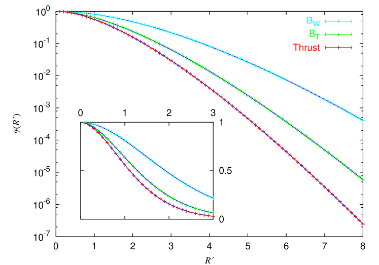
Figure 1: ${\cal{F}}(R^{\prime})$ for the thrust and the two broadenings. The lines are the analytical results, while the points are the numerical results.

3.2 $\boldsymbol{e^{+}e^{-}\to}\mbox{3 jets}$: thrust minor (a.k.a. $\boldsymbol{K_{\mathrm{out}}}$)

The procedure can also be applied to multi-jet event shapes, such as $T_{m}$ and $D$ parameter, which have been studied recently in the near-to-planar three-jet region [8, 9]. In particular, we would like to compare the numerical results to the analytical resummation of $T_{m}$ distribution, which is much more involved than that of the $D$ parameter due to hard parton recoil effects.

In the near to planar three-jet region $T\sim T_{M}\gg T_{m}$, a three-jet event consists of a hard quark-antiquark-gluon system accompanied by soft secondary partons. We denote the hard partons by $p_{1},p_{2}$ and $p_{3}$ with $p_{1}^{0}>p_{2}^{0}>p_{3}^{0}$ and call $\delta=1,2,3$ the configuration in which the gluon momentum is $p_{\delta}$. As discussed in [8], the function ${\cal{F}}_{T_{m}}(R^{\prime})$ depends on the colour configuration of the hard underlying system.

The simple observable $T_{m,s}$ is determined by (13). In terms of soft parton momenta this gives $T_{m,s}=\max_{i}\{N_{i}|k_{ix}|/Q\}$, where $k_{ix}$ is the out-of-event-plane momentum component of emitted parton $i$ and, due to the recoil kinematics, $N_{i}$ is $4$ or $2$ respectively according to whether or not emission $i$ is in the same hemisphere as the most energetic hard parton (as was shown in [8] and can easily be determined numerically as well as analytically).

The analytical result for ${\cal{F}}^{(\delta)}_{T_{m}}(R^{\prime})$ has been computed in [8]. We do not reproduce here its explicit form, since its various components involve up to as many as five nested integrals, but we plot in figure 2 the analytical results as a function of $R^{\prime}$ together with ${\cal{F}}^{(\delta)}_{T_{m}}$ obtained using the numerical procedure.

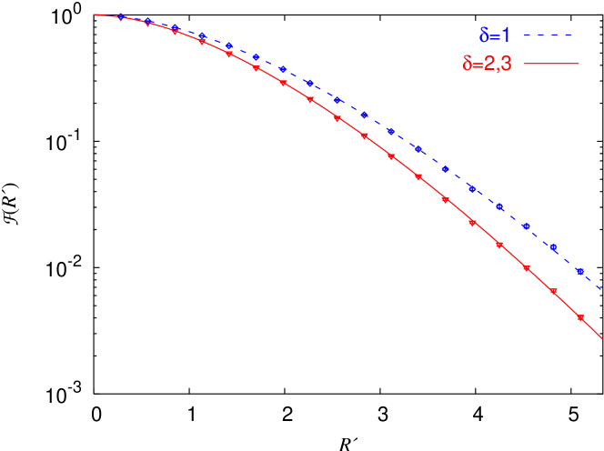
Figure 2: ${\cal{F}}^{(\delta)}(R^{\prime})$ for the thrust minor distributions in the three different colour configurations. The lines indicate the analytical results, while the points are the numerical results.

4 New results

We now exploit our method to compute the function ${\cal{F}}$ for some observables for which an analytical expression for the resummed PT distribution has not so far been found: the thrust major, the oblateness and the Durham three-jet resolution. In the first two cases we suspect that it may not even be possible to find analytical expressions.

4.1 Thrust major

The thrust major, $T_{M}$, is defined in (38). In order to compute ${\cal{F}}_{T_{M}}$ we have as the ‘simple’ observable

$$T_{M,s}\equiv 2\cdot\max_{i}\frac{|\vec{k}_{ti}|}{Q}\>.$$ (32)

Our numerical procedure gives the function ${\cal{F}}_{T_{M}}(R^{\prime})$ shown in figure 3. The resummed $T_{M}$ distribution is then given by (11), where $\Sigma_{s}(T_{M})$, defined generally in (17), is

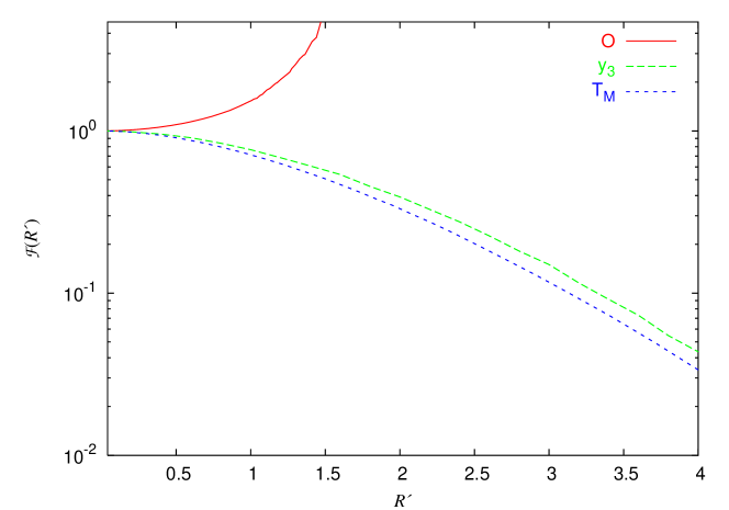
Figure 3: The function ${\cal{F}}(R^{\prime})$ for the thrust major, the oblateness and the Durham three-jet resolution.

$$\begin{split}\Sigma_{s}(T_{M})&=e^{-R_{s}(T_{M}/2)}=e^{-R_{s}(T_{M})}e^{-R^{\prime}\ln 2}\>,\\ R_{s}(T_{M})&=2C_{F}\int_{T^{2}_{M}Q^{2}}^{Q^{2}}\frac{dk_{t}^{2}}{k_{t}^{2}}\frac{\alpha_{{\textsc{s}}}(k_{t})}{\pi}\left(\ln\frac{Q}{k_{t}}-\frac{3}{4}\right)\>,\end{split}$$ (33)

i.e. it is expressed in terms of a radiator, $R_{s}(T_{M})$, which is identical to that for $B_{T}$ and $B_{W}$. Its analytical expression to SL accuracy has been already computed in [2] and is recalled in Appendix C.1.

We then match the above resummed result (using the $\log R$-matching scheme [1]) with the exact ${\cal{O}}\left(\alpha_{{\textsc{s}}}^{2}\right)$ results computed with EVENT2 [16], to give the curve shown in figure 4.

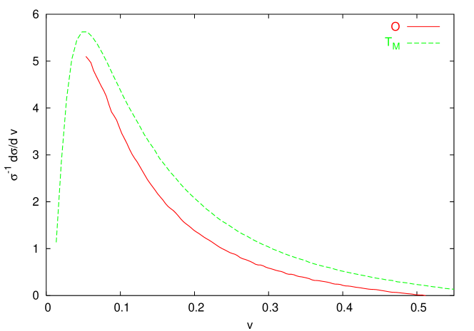
Figure 4: The full SL-resummed distributions for the thrust major and the oblateness including second order matching ($\log R$-scheme), shown for $\sqrt{s}=M_{Z}$.

4.2 Oblateness

The ‘simple’ observable (32) can be also exploited to compute ${\cal{F}}(R^{\prime})$ for the oblateness, defined as the difference between the thrust major and the thrust minor (see (40)).

The function ${\cal{F}}(R^{\prime})$ for the oblateness (also shown in figure 3) behaves quite differently from that for the other variables considered so far, since it increases rather than decreases with increasing $R^{\prime}$.

There is a simple reason for this difference. For most variables, adding an extra emission to the ensemble can only increase the value of the observable, largely because most observables essentially involve a sum of positive definite quantities.

The oblateness is unusual in that it is a difference of two quantities. For a single emission the thrust minor is zero and so the oblateness is equal to the thrust major. But as soon as one considers a second emission, there exist configurations for which the thrust minor is almost equal to the major, leading to a value for the oblateness which is smaller than that of the simple observable.

This is illustrated in figure 5 which shows the probability distribution for the ratio of the true variable to the simple one, for both the thrust major and the oblateness. The thrust major exhibits a sharp cutoff for $v/v_{s}<1$. The oblateness on the other hand has a roughly power-like tail extending to arbitrarily small values of $v/v_{s}$, originating from events with nearly identical major and minor projections. Since eq. (10) involves the ratio $(v/v_{s})^{-R^{\prime}}$, if a sufficient fraction of events has $v<v_{s}$, then ${\cal{F}}(R^{\prime})$ can be larger than $1$.

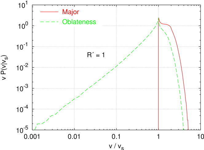
Figure 5: Distribution of the value of $v/v_{s}$ for the oblateness and the thrust major.

However ${\cal{F}}$ being larger than one is not the only consequence of the tail at small $v/v_{s}$: if $R^{\prime}$ is too large then the factor $(v/v_{s})^{-R^{\prime}}$ can completely compensate the smallness of $P(v|v_{s})$, and the integral (7) then diverges. The start of this divergence is clearly visible for the oblateness in figure 3. We shall refer to the position of the divergence as $R^{\prime}_{\mathrm{c}}$.

In the case of the oblateness, simple considerations based on two-gluon configurations suggest that $R^{\prime}_{\mathrm{c}}=2$, corresponding to a tail of $vP(v|v_{s})$ proportional to $(v/v_{s})^{2}$. This does not quite correspond to what is seen in figure 5, and it is not clear whether the actual $vP(v|v_{s})$ has a different power for the tail, or simply some extra logarithmic enhancement.

We emphasise that the divergence in ${\cal{F}}$ is not a particularity of our approach. Recently for example, such a problem has been extensively discussed in the context of the jet broadening in DIS [6], and it is in general present for all observables which can have zero value even in the presence of emissions. Physically, what happens is that for $R\simeq R^{\prime}_{\mathrm{c}}$ there is a transition from the normal double-log Sudakov suppression to some other behaviour (e.g. a suppression proportional to $v^{2}$). Such a transition is beyond representation in terms of a pure SL function, leading to a breakdown in the hierarchy of leading and subleading logs. This is seen for example in the fact that NNLL terms are even more strongly divergent that the NLL ones. In analytical resummation approaches, with considerable extra work, it is sometimes possible to include an appropriate subset of subleading terms so as to bring the answer back under control over the whole range of the $R^{\prime}$.

On the other hand as long $R^{\prime}_{\mathrm{c}}-R^{\prime}$ is of order one (formally $\gg\sqrt{\alpha_{{\textsc{s}}}}$) it can be shown that the divergence can be ignored [6]. Therefore, so as to be sure of remaining in the region under control, we suggest that the oblateness distribution be studied only for $R^{\prime}(O)<1$. This is illustrated in figure 4, which shows the full resummed matched distribution for the oblateness (based on an expression analogous to (33)). The point $R^{\prime}=1$ is just to the right of the peak region — accordingly, it should be possible to compare most, though not all the data with the resummed predictions.

4.3 Durham three-jet resolution

Now we wish to calculate the multiple emission single-logs for the distribution of the three-jet resolution parameter, $y_{3}$, in the Durham algorithm (the corresponding integrated distribution is also referred to as the two-jet rate). The leading logs, and some subleading logs (those necessary for NLL accuracy in the exponentiated answer rather than the exponent) were calculated in [13]. The NL logs associated with the appropriate scheme choice for $\alpha_{{\textsc{s}}}$ were given in [14]. However those coming from the non-trivial dependence on multiple emissions have yet to be calculated.

Jet rates differ from most event shapes in that they do not satisfy item 3 of the conditions for applicability given in appendix A, which was required for a straightforward elimination of subleading logarithms, using the event-shape specific method of section 2.4. This condition was that $V(\{k_{i}\})$ should stay invariant under certain transformations of the $k_{i}$ which kept the $\{V(k_{i})\}$ constant. It allowed phase-space integrations over rapidity to be carried out analytically.

Nevertheless we can still use the ‘general’ method for the elimination of subleading logs, as outlined in section 2.4. It requires that we be able to evaluate the observable accurately even when it takes values much smaller than the smallest machine representable (double precision) floating point number, so that we can take the limit $\alpha_{{\textsc{s}}}\to 0$ with constant $\alpha_{{\textsc{s}}}L$ (which implies $L\to\infty$).

It turns out that to succeed in doing this (without recourse to arbitrary precision arithmetic) we must carry out an analytical analysis of the observable’s dependence on multiple soft and collinear emissions. One might raise the criticism that this negates the philosophy of our numerical approach. Such a criticism would be only partially justified since in a traditional resummation approach once one has determined this dependence, one still has to understand what transformations are needed in order to write it in a factorised form (cf. the discussion in the introduction), and then one has to carry out the inverse transformations, both operations involving considerable work.

4.3.1 Soft and collinear analysis

It is useful to start by recalling the definition of the Durham jet finding algorithm [26], given in terms of a resolution parameter $y_{\mathrm{cut}}$ as follows:

1. For all pairs of (pseudo)particles $i,j$ calculate

   $$y_{ij}=\frac{2\mathrm{min}(E^{2}_{i},E_{j}^{2})(1-\cos\theta_{ij})}{Q^{2}}\,.$$ (34)

2. If all $y_{ij}>y_{\mathrm{cut}}$ stop. The number of jets is then defined to be equal to the number of (pseudo)particles left.

3. Otherwise recombine the pair with the smallest $y_{ij}$ into a single pseudoparticle (there are various schemes according to whether one wants the recombined particle to be massless, see for instance [27]).

4. Go back to step 1.

The three-jet resolution parameter, $y_{3}$, is the maximum value of $y_{\mathrm{cut}}$ that leads to a $3$-jet event.

To understand the soft and collinear limit of our observable, we shall suppose that we have an event with hard partons $a$ and $b$ and soft-collinear partons $1\ldots n$. To start with we should examine the value of the $y_{ij}$ for different kinds of pairings of particles:

• If $i$ and $a$ are in the same hemisphere $y_{ia}\simeq E_{i}^{2}\theta_{i}^{2}\simeq k_{ti}^{2}$.

• If $i$ and $j$ are in different hemispheres then $y_{ij}\simeq 4E_{<}^{2}$, where $E_{<}=\min(E_{i},E_{j})$.

• If $i$ and $j$ are in the same hemisphere then $y_{ij}\simeq E^{2}_{<}|\vec{\theta}_{i}-\vec{\theta}_{j}|^{2}$, where we define the angles as vectors in the transverse directions.

In these relations we have defined ${\vec{\theta}}_{i}$ to be the angle between parton $i$ and its nearest hard parton (the vector indicates the azimuthal direction), and $k_{ti}$ to be the relative transverse momentum. The centre of mass energy $Q$ is taken to be $1$.

To determine the value of $y_{3}$ for an arbitrary ensemble of soft and collinear particles it is beneficial to start first with some simple cases: if we have just a single emission then $y_{3}=k_{t}^{2}$ of that emission (hence the alternative name — $k_{t}$ algorithm).

Now let us consider two emissions, labelled $1$ and $2$. We take $k_{t1}>k_{t2}$, the non-trivial case being when $k_{t2}$ and $k_{t1}$ are however of the same order. We shall assume that the two emissions are widely separated in rapidity, as is appropriate when considering only NLL terms. There are then four relevant configurations, illustrated in figure 6:

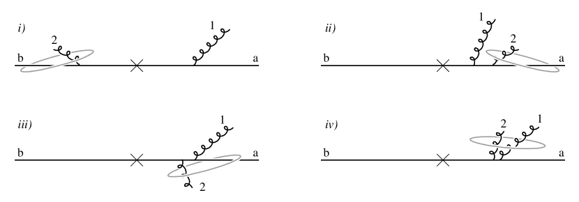
Figure 6: Representation of the clustering in the Durham algorithm, for various configurations. Both gluons are soft and collinear, with $k_{t1}>k_{t2}$ but of the same order. When they are in the same hemisphere, their angles are assumed to be strongly ordered (though for clarity only weak ordering is represented in the figure). The hoop indicates which pair of particles clusters first.

• If $1$ and $2$ are in opposite hemispheres (as in figure) then $y_{12}=4\min(E_{1}^{2},E_{2}^{2})\gg y_{1a}>y_{2b}$, so parton $2$ gets recombined with $b$. Since now the only soft-collinear parton left is $1$ we get $y_{3}=k_{t1}^{2}$.

• If $1$ and $2$ are in the same hemisphere (say the hemisphere of $a$) and $\theta_{1}\gg\theta_{2}$ (which implies $E_{1}\ll E_{2}$), then we get $y_{12}\simeq y_{1a}=k_{t1}^{2}$, while $y_{2a}=k_{t2}^{2}$ which is smaller. So once again parton 2 recombines with a hard parton and we are left with just parton 1, which then leads us to $y_{3}=k_{t1}^{2}$.

• If $1$ and $2$ are in the same hemisphere (again the hemisphere of $a$), but $\theta_{1}\ll\theta_{2}$ (which implies $E_{1}\gg E_{2}$), then we have $y_{12}\simeq y_{2a}=k_{t2}^{2}$, while $y_{1a}=k_{t1}^{2}$ which is larger. So the recombination that will take place is either $12$ or $a2$. Which one depends on whether $|\vec{\theta}_{2}-\vec{\theta}_{1}|^{2}>\theta_{2}^{2}$. If $\vec{\theta}_{1}\cdot\vec{\theta}_{2}<0$ then the inequality is satisfied, and we have a $a2$ recombination, so that just as before $y_{3}=k_{t1}^{2}$.

• If $1$ and $2$ are in the same hemisphere and $\theta_{1}\ll\theta_{2}$, as in iii), but with $\vec{\theta}_{1}\cdot\vec{\theta}_{2}>0$, then $y_{12}<y_{2a}$ and (at last a non trivial result!) we recombine partons $1$ and $2$. This gives us a pseudoparticle with the energy of parton $1$ (recall $E_{1}\gg E_{2}$) and squared transverse momentum $k_{tp}^{2}=|\vec{k}_{t1}+\vec{k}_{t2}|^{2}$. The value of $y_{3}$ is then just set by the $k_{tp}^{2}$ of the pseudoparticle. We note that since $\vec{\theta}_{1}\cdot\vec{\theta}_{2}>0$, $k_{tp}$ is always larger than $k_{t1}$.

We can see from this analysis that item 3 of the conditions for applicability in appendix A is violated: exchanging the rapidities of the two gluons, while keeping their transverse momenta and azimuths constant (i.e. exchanging configurations ii and iv), leads to a change in the value of $y_{3}$.

The above two-gluon analysis also points the way to a general algorithm suitable for taking the limit of very small values of $y_{3}$. In order to be able to represent all quantities on a computer in standard double precision we work in terms of rapidities $\eta_{i}$ and rescaled transverse momenta $\kappa_{i}=k_{ti}/\max_{j}\{k_{tj}\}$. We further assume (as is appropriate at NLL order) that particles are all widely separated in rapidity from one another. The $y_{3}$ value for the Durham jet algorithm can then be determined as follows:

1. Find the index $I$ of the smallest of the $\{\kappa_{i}\}$.

2. Considering only the soft partons $j$ in the same hemisphere as $I$ and which satisfy $\vec{\kappa}_{I}\cdot\vec{\kappa}_{j}>0$, find the index $J$ of the one with the smallest positive value of $|\eta_{j}|-|\eta_{I}|$. If there are no soft partons $j$ with both $\vec{\kappa}_{I}\cdot\vec{\kappa}_{j}>0$ and $|\eta_{j}|>|\eta_{I}|$, then let $J=a$ or $b$, according to which is the collinear hard parton.

3. If $J=a$ or $J=b$ then just throw away parton $I$. Otherwise recombine $I$ and $J$ as follows: the rapidity $\eta_{p}$ of the pseudoparticle is just set to $\eta_{J}$ (this involves a mistake on $\eta_{p}$ by an additive amount of order $1$ — but that is subleading), while its transverse momentum is the vector sum, $\vec{\kappa}_{p}=\vec{\kappa}_{I}+\vec{\kappa}_{J}$. At NLL order, this procedure is appropriate for all standard recombination schemes.

4. If only one soft pseudoparticle remains, $P$, then $y_{3}/\max_{j}\{k_{tj}^{2}\}=\kappa_{P}^{2}$. Otherwise go back to step 1.

4.3.2 Numerical results

Using the above algorithm for calculating $y_{3}$ at arbitrarily small values we can now numerically determine the function ${\cal{F}}_{y_{3}}(R^{\prime})$. The results are shown in figure 3 together with those for the thrust major and the oblateness.

For phenomenology one also needs to know the resummation for the simple observable related to $y_{3}$. Since $y_{3s}$ is just the (normalised) squared transverse momentum, $y_{3s}=k_{t}^{2}/Q^{2}$, we have from (17) and (18) that

$$\begin{split}\Sigma_{s}(y_{3})=e^{-R_{s}(y_{3})}\,,\qquad R_{s}(y_{3})=C_{F}\int_{y_{3}Q^{2}}^{Q^{2}}\frac{dk_{t}^{2}}{k_{t}^{2}}\frac{\alpha_{{\textsc{s}}}(k_{t})}{\pi}\left(\ln\frac{Q^{2}}{k_{t}^{2}}-\frac{3}{2}\right)\>.\end{split}$$ (36)

This corresponds to what was calculated in [14], which contains the explicit NLL form for the result of the integration. The full NLL resummed prediction for the Durham $y_{3}$ can then be obtained from (11), with ${\cal{F}}_{y_{3}}(R^{\prime})$ as shown in figure 3.

For completeness, in figure 7 we show the final perturbative result for the NLL resummed Durham $y_{3}$ distribution, matched to the NLO fixed order results. We choose here as a recombination scheme the $E0$ scheme (see for instance [27]), in which the energy of the recombined pseudo-particle equals the sum of the energies of the two (pseudo)-particles, while the three-momentum is rescaled so as to keep pseudo-particles massless. Choosing a different recombination scheme will affect only the large $y_{3}$ region and subleading logs. In the same figure we also show the matched resummed curve for the Cambridge algorithm [28], which is also in the ‘family’ of $k_{t}$ algorithms — however it has a different clustering sequence which leads to the property that for emissions widely separated in rapidity, the $y_{3}$ value is simply the maximum of the emitted squared transverse momenta. As a consequence ${\cal{F}}(R^{\prime})=1$, so that the full resummed distribution is simply given by $\Sigma_{s}$.

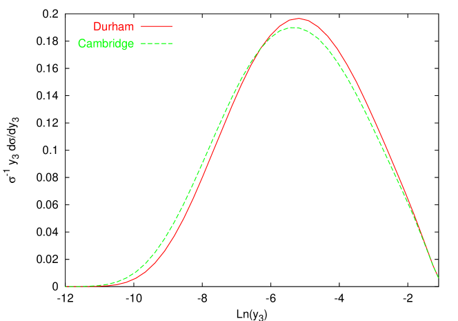
Figure 7: The full SL-resummed distributions for the Durham and Cambridge three-jet resolution $y_{3}$ including second order matching ($\log R$-scheme).

5 Conclusions

In this paper we have presented a general method for the numerical calculation of the only non-trivial class of next-to-leading logarithms in (global) event shapes. For most event shapes it means that the calculation of the resummed distribution (in the $n$-jet limit for an observable which has non-zero values only for ensembles of $n+1$ or more particles) can be reduced to the following three tasks:

• The evaluation of the dependence of the observable on a single soft and collinear emission.

• The calculation of a resummed distribution, $\Sigma_{s}$, based on that single-emission dependence, through eqs. (17) and (18) (or their extensions in situations with more than two hard ‘legs’, and/or incoming hadrons).

• The provision of a computer subroutine which calculates the value of the observable for an arbitrary set of four-momenta. One can then use the algorithm of this paper to determine a single logarithmic function ${\cal{F}}(R^{\prime})$ which accounts for the observable’s non-trivial dependence on multiple emissions, and multiplies $\Sigma_{s}$ to give the resummed distribution to full NLL accuracy.

The method thus provides both a very simple, but also general way of obtaining NLL resummed distributions for final-state observables.

As a cross check, it has been tested against a range of previously studied observables (including some in processes other than $e^{+}e^{-}$, which for brevity we have not shown here, but which are listed at the end of appendix B), and consistently reproduces the known analytical results.

It has also been applied to observables that up to now had proved beyond the scope of existing analytical methods, allowing us to present the first fully NLL resummed distributions for the thrust major, the oblateness and the three-jet resolution $y_{3}$ in the Durham algorithm. For the three-jet resolution some analytical analysis was required in order to provide a subroutine capable of giving an accurate evaluation of $y_{3}$ even in the limit of very small $y_{3}$. That analysis also has some intrinsic interest for the light it casts on the functioning of the Durham jet algorithm.

It should be emphasised that the philosophy of the approach presented here differs entirely from that of a Monte Carlo event generator (such as Herwig [29] or Pythia [30]). An event generator may well reproduce many of the leading and subleading logarithms for event shape distributions, however even at parton level there will also be contamination from potentially spurious NNLL and non-perturbative terms, and it is not currently possible to match to exact next-to-leading order calculations.

On the other hand the results produced by our algorithm are indistinguishable from those of fully analytical methods, allowing the same procedures of truncation at pure LL and NLL terms, and straightforward matching to fixed leading and NLO calculations. As such, our method is an essential development should one wish at some stage to fully automate the calculation of resummed distributions, in a manner analogous to what has become standard for fixed-order predictions of non-inclusive observables.

Appendix A Conditions for applicability

Various steps in this article rely on the observable under consideration being ‘suitable’. Here we attempt to define what is meant by this. The first two conditions are required for the exponentiation of the double logarithms. The third condition is specific to the second (event-shape specific) method for eliminating subleading effects (discussed in section 2.4):

1. If one is resumming from a Born level consisting of $n$ coloured hard partons (incoming or outgoing), then for any configuration consisting of just $n$ hard partons the observable must have a constant value $V_{0}$ independent of the hard configuration. Furthermore for a general configuration of $n+1$ hard partons the observable must have a value different from $V_{0}$. Without loss of generality, one can redefine the observable such that $V_{0}=0$.

   So for example, we can consider the thrust in the 2-jet limit, or the thrust minor in the 3-jet limit, but not the thrust-minor in the 2-jet limit, nor the thrust in the 3-jet limit.

2. If we select $m$ soft, collinear momenta (with respect to any of the $n$ hard partons) such that $V(k_{1})\sim V(k_{2})\sim\ldots\sim V(k_{m})$, then the observable must satisfy the condition $V(k_{1},\ldots,k_{m})\sim V(k_{1})$. This is necessary in order for the double logarithms to exponentiate, and excludes for example observables based on the JADE jet-clustering algorithm [31].

3. Given $m$ soft and collinear (SC) partons, the value of the observable $V(k_{1},\ldots,k_{m})$ must remain unchanged (to within corrections of relative order of the softness or collinearity) if we vary the rapidity and absolute transverse momentum (but not the azimuth) of any of the $m$ SC partons subject to the following restrictions:

   • the $V(k_{i})$ are all kept constant;

   • each SC parton remains collinear to the hard parton to which it was originally collinear.

   This condition is necessary if one is to use method 2 of section 2.4 for the elimination of subleading logs. We note that in general it is satisfied by event shapes, but not for example by the jet rate with the Durham algorithm.

In addition to the above conditions, we note that for the simple observable to have a straightforward resummation in terms of independent emissions (cf. eqs. (15), (17) and (18)) it is necessary that it be global [12].

Appendix B Definition of observables

For completeness we recall here the definition of all the event shape variables that we refer to in the main text (except for $y_{3}$ whose definition is explicitly needed in section 4.3 and so is directly given there).

• Thrust $T$, Thrust major $T_{M}$, Thrust minor $T_{m}$, Oblateness $O$

  The thrust is defined as

  $$T=\frac{1}{\sum_{i}|{\vec{p}_{i}}|}\max_{\vec{n}}\sum_{i}|\vec{p}_{i}\cdot\vec{n}|\>,$$ (37)

  where $\vec{p}_{i}$ are the three-momenta of the outgoing particles. The thrust axis is the unit vector $\vec{n}_{T}$ which maximises the sum in (37) and gives therefore the direction along which the projection of momenta is maximal.

  The thrust major is then defined similarly, but the maximisation procedure is restricted to unit vectors perpendicular to $\vec{n}_{T}$

  $$T_{M}=\frac{1}{\sum_{i}|{\vec{p}_{i}}|}\max_{\vec{n}\cdot\vec{n}_{T}=0}\sum_{i}|\vec{p}_{i}\cdot\vec{n}|\>.$$ (38)

  The vector $\vec{n}_{T_{M}}$ which maximises the sum in (38) defines the thrust major axis.

  Given the thrust and the thrust major axes, the thrust minor is defined as

  $$T_{m}=\frac{1}{\sum_{i}|{\vec{p}_{i}}|}\sum_{i}|\vec{p}_{i}\cdot\vec{n}_{T_{m}}|\>,\qquad\vec{n}_{T_{m}}=\vec{n}_{T}\times\vec{n}_{T_{M}}\>,$$ (39)

  and the oblateness as

  $$O=T_{M}-T_{m}\>.$$ (40)

• The broadenings:

  The broadenings measure the transverse size of the jets. The plane perpendicular to the thrust axis through the origin divides an event in two hemispheres, which are usually called left (L) and right (R) hemisphere. One defines first the right ($B_{R}$) and left broadening ($B_{L}$) as

  $$B_{R/L}=\frac{1}{2\>\sum_{i}|{\vec{p}_{i}}|}\sum_{i\in R/L}|\vec{p}_{ti}|\>,$$ (41)

  with $\vec{p}_{ti}=\vec{p}_{i}\times\vec{n}_{T}$.

  One can then define the total ($B_{T}$) and wide ($B_{W}$) jet broadening as

  $$\begin{split}B_{T}&=B_{R}+B_{L}\>,\\ B_{W}&=\max\{B_{R},B_{L}\}\>.\end{split}$$ (42)

As well as having been applied to the observables defined above, our method has also been successfully tested against known analytical results for several other variables: the $D$-parameter in 3-jet $e^{+}e^{-}$ events [9], the current-jet broadening (with respect to the photon axis) in $1+1$-jet DIS events [6], the out-of-plane momentum in $2+1$-jet DIS events [11] and the out-of-plane momentum for $W/Z+\mathrm{jet}$ events in hadron-hadron collisions [10].

Appendix C Analytical ingredients

Here we summarise all the analytical ingredients needed for the calculation of the resummed distributions of the three observables studied in section 4. This means NLL expressions for the simple radiators and derivatives (the formulae are all well known in the literature), as well as the fixed order expansions.

Computer subroutines which interpolate tabulated numerical values for the functions ${\cal{F}}(R^{\prime})$ are available on request from the authors, as are example programs for calculating the complete resummed, matched distributions.

C.1 Thrust major and oblateness

For the thrust major and oblateness, the simple radiator, $R_{s}$ (defined in (33)) is given to NLL order by $R_{s}(v)=Lg_{s1}(\alpha_{{\textsc{s}}}L)+g_{s2}(\alpha_{{\textsc{s}}}L)$ with

$$g_{s1}(\alpha_{{\textsc{s}}}L)=\frac{C_{F}}{\pi\beta_{0}\lambda}\left(-2\lambda-\ln(1-2\lambda)\right),$$ (43)

and

$$g_{s2}(\alpha_{{\textsc{s}}}L)=\frac{3C_{F}}{2\pi\beta_{0}}\ln(1-2\lambda)+\frac{C_{F}K}{2\pi^{2}\beta_{0}^{2}}\frac{2\lambda+(1-2\lambda)\ln(1-2\lambda)}{1-2\lambda}\\ +\frac{C_{F}\beta_{1}}{\pi\beta_{0}^{3}}\left(-\frac{2\lambda+\ln(1-2\lambda)}{1-2\lambda}-\frac{1}{2}\ln^{2}(1-2\lambda)\right),$$ (44)

where $\lambda=\alpha_{{\textsc{s}}}\beta_{0}L$ and $L=\ln 1/v$. The coefficients of the $\beta$-function are given by

$$\beta_{0}=\frac{11C_{A}-2n_{\!f}}{12\pi},\qquad\quad\beta_{1}=\frac{17C_{A}^{2}-5C_{A}n_{\!f}-3C_{F}n_{\!f}}{24\pi^{2}}\,,$$ (45)

and the constant relating the gluon Bremsstrahlung scheme [23] to the $\overline{\mbox{\scriptsize MS}}$ is

$$K=C_{A}\left(\frac{67}{18}-\frac{\pi^{2}}{6}\right)-\frac{5}{9}n_{\!f}\,.$$ (46)

Also useful is the formula for $R^{\prime}$ (at NLL equal to $R_{s}^{\prime}$):

$$R^{\prime}(v)\equiv\frac{d}{dL}(Lg_{s1}(\alpha_{{\textsc{s}}}L))=\frac{C_{F}}{\pi\beta_{0}}\frac{4\lambda}{1-2\lambda}\,.$$ (47)

For matching to fixed order calculations, it is necessary to have the coefficients of the fixed order expansion of the full resummed distribution. They are given in table 1, using the notation of [1].

$G_{12}$	=	$-4C_{F}$
$G_{11}$	=	$C_{F}\left(6-8\ln 2\right)$
$C_{1}$	=	$C_{F}\left(6\ln 2-4\ln^{2}2+\pi^{2}-\frac{17}{2}\right)$
$G_{23}$	=	$-C_{F}\left(\frac{88}{9}C_{A}-\frac{32}{9}T_{R}n_{f}\right)$
$G_{22}$	=	$C_{F}\left(64{\cal{F}}_{2}C_{F}+\left(\frac{2}{3}\pi^{2}-\frac{35}{9}-\frac{88}{3}\ln 2\right)C_{A}+\left(\frac{4}{9}+\frac{32}{3}\ln 2\right)T_{R}n_{f}\right)$

Table 1: Logarithmic coefficients $G_{nm}$ and the constant $C_{1}$ for thrust major and oblateness; for $T_{M}$ one has ${\cal{F}}_{2}=-0.46851\pm 0.00017$, for the oblateness ${\cal{F}}_{2}=0.37799\pm 0.00029$.

Tables 2a and 2b show the two subleading coefficients $G_{21}$ and $C_{2}$ for the thrust major and the oblateness respectively. They are obtained from the fixed order integrated distribution (calculated with EVENT2 [16]) after subtracting the leading and next-to-leading logs. The final errors shown are obtained by adding in quadrature the mean error and the maximal discrepancy between the mean coefficient and the coefficient obtained in a single fit. The errors are to be considered as indicative only, because of the difficulty in estimating the systematic uncertainty associated with the choice of fit range.

a) Thrust Major
Fit-range	$G_{21}$	$C_{2}$
$[-9;-5]$	$-20.3\pm 2.5$	$154.0\pm 14.8$
$[-8;-5]$	$-20.7\pm 3.3$	$156.2\pm 19.3$
$[-9;-6]$	$-21.0\pm 2.9$	$160.4\pm 19.2$
	$-20.6\pm 2.9$	$156.9\pm 18.1$

b) Oblateness
Fit-range	$G_{21}$	$C_{2}$
$[-8;-4]$	$75.3\pm 1.0$	$166.1\pm 4.6$
$[-7;-4]$	$75.6\pm 1.1$	$164.9\pm 5.3$
$[-8;-5]$	$70.8\pm 2.9$	$191.6\pm 16.5$
	$73.9\pm 3.5$	$174.2\pm 19.5$

Table 2: Fits of $G_{21}$ and $C_{2}$ for the thrust major and the oblateness.

C.2 Three-jet resolution

For the Durham (and Cambridge) three jet resolution parameter, the simple radiator, $R_{s}$, defined in (36), is given to NLL order by $R_{s}(v)=Lg_{s1}(\alpha_{{\textsc{s}}}L)+g_{s2}(\alpha_{{\textsc{s}}}L)$ with

$$g_{s1}(\lambda)=\frac{C_{F}}{\pi\beta_{0}\lambda}\left[-\lambda-\ln{(1-\lambda)}\right]\,,$$ (48)

$$g_{s2}({\lambda})=\frac{3C_{F}}{2\pi\beta_{0}}\ln(1-\lambda)+\frac{KC_{F}[\lambda+(1-\lambda)\ln(1-\lambda)]}{2\pi^{2}\beta_{0}^{2}(1-\lambda)}\\ +\frac{C_{F}\beta_{1}}{\pi\beta_{0}^{3}}\left[-\frac{\lambda+\ln(1-\lambda)}{1-\lambda}-\frac{1}{2}\ln^{2}{(1-\lambda)}\right],$$ (49)

and, as before, $\lambda=\alpha_{{\textsc{s}}}\beta_{0}L$. $R^{\prime}$ is given by

$$R^{\prime}=\frac{C_{F}}{\pi\beta_{0}}\frac{\lambda}{1-\lambda}\,.$$ (50)

The coefficients of the fixed order expansion of the resummation are given in table 3.

$G_{12}$	=	$-C_{F}$
$G_{11}$	=	$3C_{F}$
$C_{1}$	=	$C_{F}\left(-6\ln 2+\frac{\pi^{2}}{6}-\frac{5}{2}\right)$
$G_{23}$	=	$-C_{F}\left(\frac{11}{9}C_{A}-\frac{4}{9}T_{R}n_{f}\right)$
$G_{22}$	=	$C_{F}\left(4{\cal{F}}_{2}C_{F}+\left(\frac{1}{6}\pi^{2}-\frac{35}{36}\right)C_{A}+\frac{T_{R}n_{f}}{9}\right)$

Table 3: Logarithmic coefficients $G_{nm}$ and the constant $C_{1}$ for the three-jet resolution parameter. In the Durham algorithm ${\cal{F}}_{2}=-\pi^{2}/32$, while in the Cambridge algorithm ${\cal{F}}_{2}=0$.

From fixed order results we also extract the subleading coefficients, shown in tables 4a and 4b for the Durham and Cambridge algorithms respectively. We follow the same fit procedure as for the thrust major and the oblateness. Note that these coefficients are obtained in the $E0$-scheme (see for example [27]), and that choosing a different recombination scheme will affect their value.

a) Durham
Fit-range	$G_{21}$	$C_{2}$
$[-13;-8]$	$-7.4\pm 0.1$	$19.3\pm 1.0$
$[-13;-9]$	$-7.0\pm 0.1$	$15.8\pm 1.3$
$[-12;-8]$	$-7.4\pm 0.1$	$19.4\pm 1.1$
	$-7.2\pm 0.3$	$18.2\pm 2.6$

b) Cambridge
Fit-range	$G_{21}$	$C_{2}$
$[-13;-8]$	$1.9\pm 0.1$	$-30.5\pm 1.2$
$[-13;-9]$	$2.3\pm 0.2$	$-34.1\pm 1.6$
$[-12;-8]$	$1.9\pm 0.2$	$-30.3\pm 1.4$
	$2.1\pm 0.3$	$-31.6\pm 2.9$

Table 4: The coefficients $G_{21}$ and $C_{2}$ for the three-jet resolution in the Durham and Cambridge algorithms.

References

-
[1]
S. Catani, L. Trentadue, G. Turnock and B. R. Webber,
Nucl. Phys. B 407 (1993) 3;
S. Catani, L. Trentadue, G. Turnock and B. R. Webber, Phys. Lett. B 263 (1991) 491. - [2] S. Catani, G. Turnock and B. R. Webber, Phys. Lett. B 295 (1992) 269.
-
[3]
S. Catani and B. R. Webber,
Phys. Lett. B 427 (1998) 377
[hep-ph/9801350];
S. Catani and B. R. Webber, JHEP 9710 (1997) 005 [hep-ph/9710333]. - [4] Yu. L. Dokshitzer, A. Lucenti, G. Marchesini and G. P. Salam, JHEP 9801 (1998) 011 [hep-ph/9801324].
- [5] V. Antonelli, M. Dasgupta and G. P. Salam, JHEP 0002 (2000) 001 [hep-ph/9912488].
- [6] M. Dasgupta and G. P. Salam, hep-ph/0110213.
- [7] S. J. Burby and E. W. N. Glover, JHEP 0104 (2001) 029 [hep-ph/0101226].
- [8] A. Banfi, G. Marchesini, Yu. L. Dokshitzer and G. Zanderighi, JHEP 0007 (2000) 002 [hep-ph/0004027].
- [9] A. Banfi, Yu. L. Dokshitzer, G. Marchesini and G. Zanderighi, JHEP 0150 (2001) 040 [hep-ph/0104162].
- [10] A. Banfi, G. Marchesini, G. Smye and G. Zanderighi, JHEP 0108 (2001) 047 [hep-ph/0106278].
- [11] A. Banfi, G. Marchesini, G. Smye and G. Zanderighi, JHEP 0111 (2001) 066 [hep-ph/0111157].
- [12] M. Dasgupta and G. P. Salam, Phys. Lett. B 512 (2001) 323 [hep-ph/0104277].
-
[13]
S. Catani, Yu. L. Dokshitzer, F. Fiorani and B. R. Webber,
Nucl. Phys. B 377 (1992) 445;
S. Catani, Yu. L. Dokshitzer and B. R. Webber, Phys. Lett. B 322 (1994) 263. - [14] G. Dissertori and M. Schmelling, Phys. Lett. B 361 (1995) 167.
- [15] S. J. Burby, Phys. Lett. B 453 (1999) 54 [hep-ph/9902305].
- [16] S. Catani and M. H. Seymour, Phys. Lett. B 378 (1996) 287 [hep-ph/9602277]; S. Catani and M. H. Seymour, Nucl. Phys. B 485 (1997) 291 [hep-ph/9605323].
- [17] W. T. Giele, E. W. Glover and D. A. Kosower, Nucl. Phys. B 403 (1993) 633 [hep-ph/9302225].
- [18] D. Graudenz, hep-ph/9710244.
-
[19]
Z. Nagy and Z. Trocsanyi,
Phys. Rev. D 59 (1999) 014020
[Erratum-ibid. D 62 (1999) 099902]
[hep-ph/9806317];
Z. Nagy and Z. Trocsanyi, Phys. Rev. Lett. 87 (2001) 082001 [hep-ph/0104315]. - [20] J. M. Campbell, M. A. Cullen and E. W. Glover, Eur. Phys. J. C 9 (1999) 245 [hep-ph/9809429].
- [21] A. Signer, Comput. Phys. Commun. 106 (1997) 125.
- [22] S. Weinzierl and D. A. Kosower, Phys. Rev. D 60 (1999) 054028 [hep-ph/9901277].
-
[23]
S. Catani, G. Marchesini and B. R. Webber,
Nucl. Phys. B 349 (1991) 635;
Yu. L. Dokshitzer, V. A. Khoze and S. I. Troyan, Phys. Rev. D 53 (1996) 89 [hep-ph/9506425]. - [24] C. F. Berger, T. Kucs and G. Sterman, hep-ph/0110004.
-
[25]
E. Gardi and J. Rathsman,
Nucl. Phys. B 609 (2001) 123
[hep-ph/0103217];
E. Gardi and G. Grunberg, JHEP 9911 (1999) 016 [hep-ph/9908458]. - [26] S. Catani, Yu. L. Dokshitzer, M. Olsson, G. Turnock and B. R. Webber, Phys. Lett. B 269 (1991) 432.
- [27] W. Bartel et al. [JADE Collaboration], Z. Phys. C 33 (1986) 23.
- [28] Yu.L. Dokshitzer, G.D. Leder, S. Moretti, B.R. Webber, JHEP 9708 (1997) 001 [hep-ph/9707323].
- [29] G. Marchesini, B. R. Webber, G. Abbiendi, I. G. Knowles, M. H. Seymour and L. Stanco, Comput. Phys. Commun. 67 (1992) 465.
- [30] T. Sjostrand, Comput. Phys. Commun. 82 (1994) 74.
-
[31]
N. Brown and W. J. Stirling,
Phys. Lett. B 252 (1990) 657;
S. Catani, CERN-TH-6281-91, Invited talk given at 17th Workshop of INFN Eloisatron Project, QCD at 200-TeV, Erice, Italy, Jun 11-17, 1991, Ettore Majorana Int. Sci. Ser., Phys. Sci. 60 21-41;
G. Leder, Nucl. Phys. B 497 (1997) 334 [hep-ph/9610552].