UT-978

Proton Decay in the Semi-Simple Unification

Masaaki Fujii and T. Watari

Department of Physics, University of Tokyo,
Tokyo 113-0033, Japan

Introduction

Supersymmetric(SUSY) SU(5)_GUT grand unification theories(GUT’s) are supported by the approximate SU(5)_GUT unification at around $10^{16}{\rm GeV}$ of the three gauge coupling constants of the minimal supersymmetric standard model(MSSM)[1]. However, the conceptual beauties of the GUT’s[2] and such a phenomenological success are not more than indirect evidences, and it would be the proton decay signals that makes us believe the GUT’s in nature.

The minimal SU(5)_GUT model predicts proton decay through dimension 5 operators[3], and is now almost excluded[4] by experimental bounds such as $\tau(p\rightarrow K^{+}\bar{\nu})\mathop{}_{\textstyle\sim}^{\textstyle>}6.7\times 10^{32}{\rm yr}.$(90 % C.L.)[5]. Therefore, we have to analyze the proton decay in an extended model in which those operators are suppressed or absent. Predictions on the proton decay through dimension 6 operators severely depend on how a model is extended; the life time of the proton depends on the fourth power of the mass of SU(5)_GUT-off-diagonal gauge boson (GUT gauge boson), and hence on the detailed spectrum of the model around the GUT scale. Therefore, an analysis on the proton decay has to be based on a phenomenologically reliable model of the GUT’s.

The doublet-triplet splitting problem[7] and suppression of the dimension 5 proton decay operators had been the two major obstacles in model buildings of the GUT’s. The semi-simple unification[8, 9, 10] is a model that solves these two problems in a natural way. In this letter, we calculate the proton decay rate in this model. The proton decay is relatively fast in this model, whose reason will be clear in the text. We restrict ourselves in parameter region of the model where a perturbative analysis is valid. As a result of a full next-to-leading order analysis[11], we found that the mass of the GUT gauge boson can be determined, and that the resulting life time of proton does not depend on SUSY breaking parameters so much: the life time is $\tau\simeq(3-10)\times 10^{34}{\rm{yr}}$. Various sources of uncertainties in this prediction are summarized at the end of this letter. This result means that the proton decay is generically detectable in the next-generation water Čerenkov detectors such as Hyper-Kamiokande and TITAND [12, 13].

Brief Review of the Semi-Simple Unification Model

We briefly review the semi-simple unification model that uses $\mathop{\rm SU}(5)_{\rm GUT}\times\mathop{\rm U}(3)_{\rm H}$ gauge group. This gauge group is directly broken down to the $\mathop{\rm SU}(3)_{\rm C}\times\mathop{\rm SU}(2)_{\rm L}\times\mathop{\rm U}(1)_{\rm Y}$ of the MSSM. Quark and lepton (${\bf 5^{*}+10}$) and Higgs ($H^{i}({\bf 5})+\bar{H}_{i}({\bf 5}^{*})$) supermultiplets are singlets of the $\mathop{\rm U}(3)_{\rm H}$ gauge group and transform under the $\mathop{\rm SU}(5)_{\rm GUT}$ as in the standard $\mathop{\rm SU}(5)_{\rm GUT}$ model. Some more fields are required for the GUT symmetry breaking: $X^{\alpha}_{\;\;\beta}(\alpha,\beta=1,2,3)$ transforming as (${\bf 1}$,adj.=${\bf 8}+{\bf 1}$) under the $\mathop{\rm SU}(5)_{\rm GUT}\times\mathop{\rm U}(3)_{\rm H}$ gauge group, and $Q^{\alpha}_{\;i}(i=1,\cdots,5)+Q^{\alpha}_{\;6}$ and $\bar{Q}^{i}_{\;\alpha}(i=1,\cdots,5)+\bar{Q}^{6}_{\;\alpha}$ transforming as (${\bf 5}^{*}$ + ${\bf 1}$,${\bf 3}$) and (${\bf 5+1}$,${\bf 3}^{*}$). Indices $\alpha$ and $\beta$ are for the $\mathop{\rm U}(3)_{\rm H}$ and $i$ for the $\mathop{\rm SU}(5)_{\rm GUT}$. $X^{\alpha}_{\;\;\beta}$ is also expressed as $X^{c}(t_{c})^{\alpha}_{\;\;\beta}(c=0,1-8)$, where $t^{a}(a=1-8)$ are Gell’mann matrices and $t_{0}\equiv{\bf 1}_{3\times 3}/\sqrt{6}$. Superpotential is given as[10]

$$W = \sqrt{2}\lambda_{\rm 3H}\bar{Q}^{i}_{\;\alpha}X^{a}(t_{a})^{\alpha}_{\;\beta}Q^{\beta}_{\;i}+\sqrt{2}\lambda_{\rm 3H}^{\prime}\bar{Q}^{6}_{\;\alpha}X^{a}(t_{a})^{\alpha}_{\;\beta}Q^{\beta}_{\;6}$$

$$+\sqrt{2}\lambda_{\rm 1H}\bar{Q}^{i}_{\;\alpha}X^{0}(t_{0})^{\alpha}_{\;\beta}Q^{\beta}_{\;i}+\sqrt{2}\lambda_{\rm 1H}^{\prime}\bar{Q}^{6}_{\;\alpha}X^{0}(t_{0})^{\alpha}_{\;\beta}Q^{\beta}_{\;6}$$

$$-\sqrt{2}\lambda_{\rm 1H}v^{2}X^{\alpha}_{\;\alpha}$$

$$+h^{\prime}\bar{H}_{i}\bar{Q}^{i}_{\;\alpha}Q^{\alpha}_{\;6}+h\bar{Q}^{6}_{\;\alpha}Q^{\alpha}_{\;i}H^{i}$$

$$+y_{\bf 10}{\bf 10}\cdot{\bf 10}\cdot H+y_{\bf 5^{*}}{\bf 5}^{*}\cdot{\bf 10}\cdot\bar{H}+\cdots,$$

where the parameter $v$ is of order of the GUT scale, $y_{\bf 10},y_{\bf 5^{*}}$ are Yukawa coupling constants of the quarks and leptons, and $\lambda_{\rm 3H},\lambda_{\rm 3H}^{\prime},\lambda_{\rm 1H},\lambda_{\rm 1H}^{\prime},h^{\prime},h$ are dimensionless coupling constants. One can see that the above superpotential has ${\bf Z}_{4}$ R symmetry under a charge assignment given in Table 1, and this symmetry forbids enormous mass term $W=\bar{H}H$ for the Higgs doublets. The bifundamental representation $Q^{\alpha}_{\;i}$ and $\bar{Q}^{i}_{\;\alpha}$ acquire vacuum expectation value, $\left\langle{Q^{\alpha}_{\;\;i}}\right\rangle=v\delta^{\alpha}_{i}$ and $\langle$ $\bar{Q}^{i}_{\;\;\alpha}$ $\rangle$ $=v\delta^{i}_{\alpha}$, because of the second and the third line in (S0.Ex4). Then, the mass terms of the colored Higgs multiplets arise from the fourth line in (S0.Ex4) in the GUT-breaking vacuum. The ${\bf Z}_{4}$ R symmetry is not broken even after the GUT symmetry is broken. One can also see that this ${\bf Z}_{4}$ R symmetry forbids the dangerous dimension 5 proton decay operators $W={\bf 10}\cdot{\bf 10}\cdot{\bf 10}\cdot{\bf 5}^{*}$.

Naive Estimation

At tree level, the gauge coupling constants of the $\mathop{\rm SU}(3)_{\rm C}\times\mathop{\rm SU}(2)_{\rm L}\times\mathop{\rm U}(1)_{\rm Y}$ are given in terms of those of the $\mathop{\rm SU}(5)_{\rm GUT}\times\mathop{\rm U}(3)_{\rm H}$ as :

$$\left(\frac{1}{\alpha_{3}}\equiv\frac{1}{\alpha_{C}}\right)=\frac{1}{\alpha_{\rm GUT}}+\frac{1}{\alpha_{\rm 3H}},$$ (2)

$$\left(\frac{1}{\alpha_{2}}\equiv\frac{1}{\alpha_{L}}\right)=\frac{1}{\alpha_{\rm GUT}}\quad\quad\quad$$ (3)

and

$$\left(\frac{1}{\alpha_{1}}\equiv\frac{3/5}{\alpha_{Y}}\right)=\frac{1}{\alpha_{\rm GUT}}+\frac{2/5}{\alpha_{\rm 1H}},$$ (4)

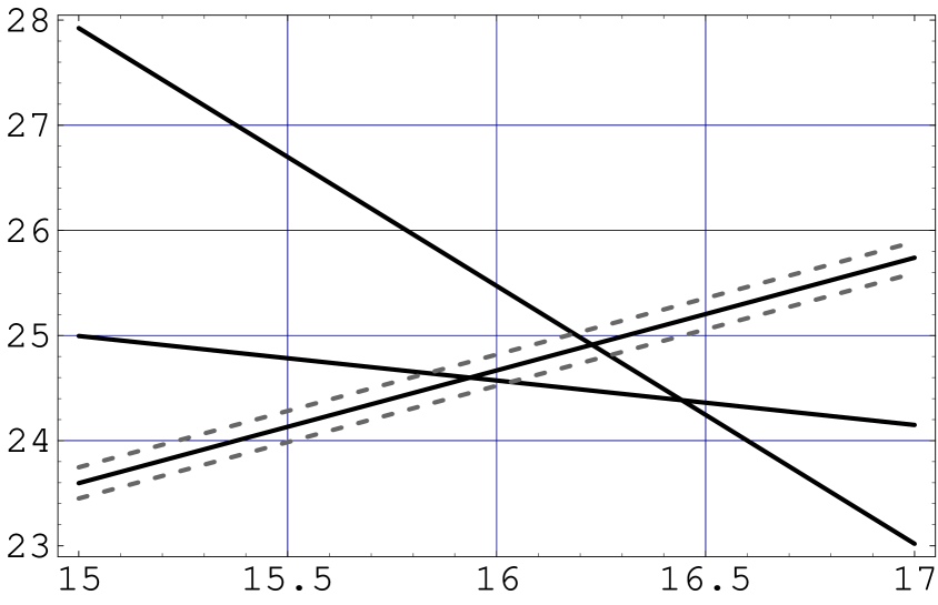
Figure 1: Approximate SU(5)_GUT relation between the three MSSM gauge coupling constants and deviation from it. 1$\sigma$ error bar of the QCD coupling are also described. SUSY threshold corrections are calculated using the spectrum of mSUGRA model with $m_{0}=250{\rm GeV}$, $M_{1/2}=500{\rm GeV}$, $A_{0}=0$ and $\tan\beta=10$. The sign of $\mu$-term is taken to be negative.

where $\alpha_{C},\alpha_{L},\alpha_{Y},\alpha_{\rm GUT},\alpha_{\rm 3H}$ and $\alpha_{\rm 1H}$ are fine structure constants of the three MSSM gauge groups, $\mathop{\rm SU}(5)_{\rm GUT}$, $\mathop{\rm SU}(3)_{\rm H}$ and $\mathop{\rm U}(1)_{\rm H}$, respectively. The approximate SU(5)_GUT relation and deviation form it (Fig.1) are naturally explained through the above equations if $1/\alpha_{\rm GUT}\sim 24$ and $1/\alpha_{3H}\mathop{}_{\textstyle\sim}^{\textstyle<}1,1/\alpha_{1H}\mathop{}_{\textstyle\sim}^{\textstyle<}2.5$. At the same time, we notice that the “GUT scale”, an energy scale at which Eqs.(2-4) hold, lies lower than the $\alpha_{1}$ - $\alpha_{2}$ unification scale $M_{1-2}$ and higher than the $\alpha_{2}$ - $\alpha_{3}$ unification scale $M_{2-3}$. Therefore, the decay rate of proton is expected to be enhanced compared with the rate using the $M_{1-2}$ as the GUT gauge boson mass.

At one-loop order, the gauge coupling of the $\mathop{\rm U}(1)_{\rm H}$ runs asymptotic non-free :

$$\frac{\partial}{\partial\ln\mu}\left(\frac{1}{\alpha_{\rm 1H}}(\mu)\right)=-\frac{6}{2\pi}.$$ (5)

There are two important remarks here. First, the cut-off scale $\Lambda$ of this model exists below the Planck scale; $1/\alpha_{\rm 1H}$ should be positive even at the $\Lambda$. The constraint $1/\alpha_{\rm 1H}\mathop{}_{\textstyle\sim}^{\textstyle<}2.5$ at the “GUT scale” allows the $\Lambda$ to be higher than the “GUT scale” by one order of magnitude or a little bit more, and this is much enough to justify the field theoretical description of the GUT symmetry breaking and to accommodate all the GUT spectrum below the cut-off scale $\Lambda$. This $\Lambda$ lies around $10^{17}{\rm GeV}$ or a little higher, though it may be below $10^{18}{\rm GeV}$. Secondly, the IR-free (asymptotic non-free) behavior of the $\mathop{\rm U}(1)_{\rm H}$ coupling leads to

$$\frac{1}{\alpha_{\rm 3H}}\ll\frac{1}{\alpha_{\rm 1H}}$$ (6)

at the “GUT scale” under an assumption

$$\frac{1}{\alpha_{\rm 3H}}(\Lambda)\simeq\frac{1}{\alpha_{1H}}(\Lambda).$$ (7)

This $\mathop{\rm U}(3)_{\rm H}$-relation at $\Lambda$ is quite natural if there is $\mathop{\rm U}(3)_{\rm H}$-structure in a fundamental theory [15]. Then, as a consequence of the relation Eq.(6), we notice that the “GUT scale” is closer to the $M_{2-3}$ rather than to the $M_{1-2}$ since $(1/\alpha_{1}-1/\alpha_{2})>(1/\alpha_{3}-1/\alpha_{2})$ there, and hence the proton decay is relatively fast.

Threshold Corrections at the GUT Scale

In the analysis at the next-to-leading order, one-loop threshold corrections of the GUT model are also taken into account. The three MSSM gauge coupling constants just below the GUT scale are expressed in terms of the gauge coupling constants and various masses in the spectrum of the GUT model, including the mass of the GUT gauge boson, $M_{v}$. Particle spectrum around the GUT scale is summarized in Table 2. Explicit expressions of the MSSM gauge coupling constants are given as follows :

$$\frac{1}{\alpha_{3}}(\mu)=\frac{1}{\alpha_{\rm GUT}}(\Lambda)+\frac{1}{\alpha_{\rm 3H}}(\Lambda)+\frac{-3}{2\pi}\ln\left(\frac{\Lambda}{\mu}\right)+\frac{1}{2\pi}\ln\left(\frac{\Lambda^{2}}{M_{\bar{c}}M_{c}}\right)-\frac{4}{2\pi}\ln\left(\frac{\Lambda}{M_{v}}\right)+\frac{6}{2\pi}\ln\left(\frac{M_{8v}}{M_{8c}}\right),$$

(8)

$$\frac{1}{\alpha_{2}}(\mu)=\frac{1}{\alpha_{\rm GUT}}(\Lambda)\quad\qquad\quad\;\;+\frac{1}{2\pi}\ln\left(\frac{\Lambda}{\mu}\right)\qquad\qquad\qquad\qquad\;\;-\frac{6}{2\pi}\ln\left(\frac{\Lambda}{M_{v}}\right),$$ (9)

$$\frac{1}{\alpha_{1}}(\mu)=\frac{1}{\alpha_{\rm GUT}}(\Lambda)+\frac{2/5}{\alpha_{\rm 1H}}(\Lambda)+\frac{33/5}{2\pi}\ln\left(\frac{\Lambda}{\mu}\right)+\frac{2/5}{2\pi}\ln\left(\frac{\Lambda^{2}}{M_{\bar{c}}M_{c}}\right)-\frac{10}{2\pi}\ln\left(\frac{\Lambda}{M_{v}}\right),\qquad\qquad\qquad$$ (10)

where $\mu$ is a renormalization point, which is taken to be just below the GUT scale, $M_{v}$, $M_{c}$, $M_{\bar{c}}$, $M_{8v}$, $M_{8c}$ are masses of particles around the GUT scale (see Table 2) and $\alpha_{\rm GUT,3H,1H}(\Lambda)$ are fine structure constants of the gauge groups $\mathop{\rm SU}(5)_{\rm GUT},\mathop{\rm SU}(3)_{\rm H}$ and $\mathop{\rm U}(1)_{\rm H}$, respectively, at the cut-off scale $\Lambda$.

In general, it is impossible to determine the $M_{v}$ if GUT models have more than three parameters. However, it is not necessarily the case in the semi-simple unification model. Threshold corrections in Eqs.(S0.Ex5-10) is simplified considerably under two reasonable assumptions. One is the $\mathop{\rm U}(3)_{\rm H}$-relation Eq.(7) and the other is ${\cal N}=2$-SUSY-relation:

$$g_{\rm 1H}\simeq\lambda_{\rm 1H}(\sim\lambda_{\rm 1H}^{\prime}),\qquad\qquad g_{\rm 3H}\simeq\lambda_{\rm 3H}(\sim\lambda_{\rm 3H}^{\prime}).$$ (11)

Under the latter condition, a large threshold correction from the massive $\mathop{\rm SU}(3)_{\rm H}$ vector multiplet is almost canceled by its ${\cal N}=2$-partner, the $\mathop{\rm SU}(3)_{\rm C}$-${\bf adj.}$ chiral multiplets, since $M_{8v}\simeq M_{8c}$. Now that the threshold corrections form the $\mathop{\rm SU}(3)_{\rm C}$-${\bf adj.}$ multiplets decouple from Eqs.(S0.Ex5-10), we are left only with two threshold corrections: one from the massive vector multiplet of the GUT gauge boson and the other from colored Higgs chiral multiplets. Then, one can easily see that three combinations,

$$\frac{1}{\alpha_{\rm GUT}}(\Lambda),\quad\ln\left(\frac{\Lambda}{M_{v}}\right){\rm~{}~{}and~{}~{}}\frac{1}{\alpha_{\rm 3H}}(\Lambda)+\frac{1}{2\pi}\ln\left(\frac{\Lambda^{2}}{M_{\bar{c}}M_{c}}\right),$$ (12)

are determined in terms of the values to be put in the LHS’s and deviation from the $\mathop{\rm U}(3)_{\rm H}$-relation and the ${\cal N}=2$-relation, once the cut-off scale $\Lambda$ is fixed.

In particular, the GUT gauge boson mass is given by

$$M_{v}=\sqrt{\frac{\mu^{3}}{\Lambda}}\exp\left(-\frac{2\pi}{24}\left(\frac{2}{\alpha_{3}}+\frac{3}{\alpha_{2}}-\frac{5}{\alpha_{1}}\right)(\mu)\right)\sqrt{\frac{M_{8v}}{M_{8c}}}\exp\left(-\frac{2\pi}{12}\left(\frac{1}{\alpha_{\rm 1H}}-\frac{1}{\alpha_{\rm 3H}}\right)(\Lambda)\right).$$ (13)

The last two factors show how the result is changed due to the deviation from the assumptions we made. $\Lambda^{-1/2}$-dependence is a direct consequence of the one-loop running of the $\alpha_{\rm 1H}$ in Eq.(5), and this negative power dependence implies that this gauge boson mass is generically light. The life time of proton through this GUT gauge boson exchange is given in terms of the $M_{v}$ as[11]

$$\tau(p\rightarrow\pi^{0}e^{+})\simeq 0.61\times 10^{35}\times\left(\frac{M_{v}}{10^{16}{\rm GeV}}\right)^{4}\left(\frac{1}{24\alpha_{\rm GUT}(M_{v})}\right)^{2}\left(\frac{0.15({\rm GeV})^{2}}{|W|}\right)^{2}{\rm yr.},$$ (14)

where $W$ is a hadron matrix element calculated with lattice quenched QCD[16].

Threshold Corrections at the Weak Scale and Two-Loop Running

In order to determine the precise value of the GUT gauge boson mass by using (13), we must accurately determine the three MSSM gauge coupling constants at the GUT scale. For this purpose, we take full one-loop threshold corrections at the weak scale into account for the three gauge coupling constants and top- and bottom-Yukawa coupling constants by following the method in Ref. [17], and use two-loop renormalization group(RG) equations. For illustration, let us briefly review the procedures which we adopt in this letter. The conventions of SUSY breaking parameters and of the sign of the $\mu$-term are the same as those in Ref. [17].

The SUSY threshold corrections to fix the $\overline{{\rm{DR}}}$ coupling $\alpha_{3}(M_{Z})$ is very simple and the result is as follows:

$$\alpha_{3}(M_{Z})=\frac{\alpha_{3}(M_{Z})_{\overline{\rm{MS}}}}{1-\Delta\alpha_{3}},$$ (15)

where

$$\Delta\alpha_{3}=\frac{\alpha_{3}(M_{Z})_{\overline{\rm{MS}}}}{2\pi}\left[\frac{1}{2}-\frac{2}{3}{\rm{ln}}\left(\frac{m_{t}}{2}\right)-2{\rm{ln}}\left(\frac{m_{\tilde{g}}}{M_{Z}}\right)-\frac{1}{6}\sum_{\tilde{q}}\sum_{i=1}^{2}{\rm{ln}}\left(\frac{m_{\tilde{q}_{i}}}{M_{Z}}\right)\right].$$ (16)

Here, $M_{Z}=91.188{\rm GeV}$ is the Z-boson pole mass and we take $\alpha_{3}(M_{Z})_{\overline{\rm{MS}}}=0.118(2)$ [20]. The summation with $\tilde{q}$ runs over all the six squark flavors, and the constant contribution $1/2$ in Eq.(16) is necessary when the coupling is translated from the $\overline{\rm MS}$ scheme to the $\overline{\rm DR}$ scheme.

Because of the breaking effects of the SU$(2)_{\rm{L}}$ gauge group, the determinations of the $\overline{\rm{DR}}$ gauge coupling constants $\alpha_{\rm Y}(M_{Z})$ and $\alpha_{\rm L}(M_{Z})$ are much more complicated. First, we calculate the $\overline{\rm{DR}}$ electromagnetic coupling constant, $\alpha(M_{Z})$. The explicit formula is given by

$$\alpha(M_{Z})=\frac{\alpha_{\rm{em}}}{1-\Delta\alpha},\qquad\alpha_{{\rm{em}}}=\frac{1}{137.036},$$ (17)

where

$$\Delta\alpha=0.0682\pm 0.0007$$

$$\hskip 22.76228pt-\frac{\alpha_{\rm{em}}}{2\pi}\left[\begin{array}[]{lll}\displaystyle{-7{\rm{ln}}\left(\frac{M_{W}}{M_{Z}}\right)+\frac{16}{9}{\rm{ln}}\left(\frac{m_{t}}{M_{Z}}\right)+\frac{1}{3}{\rm{ln}}\left(\frac{m_{H^{+}}}{M_{Z}}\right)+\frac{4}{9}\sum_{u}\sum_{i=1}^{2}{\rm{ln}}\left(\frac{m_{\tilde{u}_{i}}}{M_{Z}}\right)}\\ \displaystyle{+\frac{1}{9}\sum_{d}\sum_{i=1}^{2}{\rm{ln}}\left(\frac{m_{\tilde{d}_{i}}}{M_{Z}}\right)+\frac{1}{3}\sum_{e}\sum_{i=1}^{2}{\rm{ln}}\left(\frac{m_{\tilde{e}_{i}}}{M_{Z}}\right)+\frac{4}{3}\sum_{i=1}^{2}{\rm{ln}}\left(\frac{m_{\tilde{\chi}^{+}}}{M_{Z}}\right)}\end{array}\right].$$ (20)

Here, $\sum_{u}$ denotes a sum over $u,\;c,\;t,$ and similarly for $\sum_{d}$ and $\sum_{e}$. The numerical values appearing in the above expression includes the two-loop QED and QCD corrections in Ref. [18], as well as the five-flavor contributions in Ref. [19].

Next, we need to fix the $\overline{\rm{DR}}$ weak mixing angle $\theta_{\rm{ew}}$ to derive the $\overline{\rm{DR}}$ gauge coupling constants, $\alpha_{\rm Y}(M_{Z})$ and $\alpha_{\rm L}(M_{Z})$. The formula to get the $\overline{\rm{DR}}$ weak mixing angle is given by

$${\rm{cos}}^{2}(\theta_{\rm{ew}}){\rm{sin}}^{2}(\theta_{\rm{ew}}) = \frac{\pi\alpha(M_{Z})}{\sqrt{2}M_{Z}^{2}G_{\mu}(1-\Delta r)}\;,$$ (21)

$$\Delta r = \rho\frac{\Pi_{WW}^{T}(0)}{M_{W}^{2}}-{\cal{R}}e\frac{\Pi_{ZZ}^{T}(M_{Z}^{2})}{M_{Z}^{2}}+\delta_{VB}\;,$$ (22)

where $M_{W}=80.419{\rm GeV}$ is the W-boson pole mass, $\rho$ is defined as $\rho\equiv M_{W}^{2}/({\rm{cos}}^{2}(\theta_{\rm{ew}})M_{Z}^{2})$, $G_{\mu}=1.16639\times 10^{-5}{\rm GeV}^{-2}$ is the Fermi constant, and $\delta_{VB}$ denotes the nonuniversal vertex and box diagram corrections. The explicit formulae to calculate the quantities given in the above expressions and the $\overline{\rm{DR}}$ Yukawa coupling constants are all given in Ref. [17].

Taking $\alpha_{{\rm{em}}}$, $\alpha_{3}(M_{Z})_{\overline{\rm{MS}}}$, the quark and lepton masses, and SUSY particle masses as inputs, we calculate all the three gauge coupling constants and top- and bottom-Yukawa coupling constants in $\overline{\rm{DR}}$ scheme at the Z-boson pole mass with full one-loop threshold corrections. With these values and tree level tau-Yukawa coupling, we use the two-loop RG equations to obtain the gauge coupling constants at the GUT scale. For the Yukawa coupling constants, we use one-loop RG equations.

In this letter, we adopt the central values given in Ref. [20] for the masses of vector bosons, quarks and leptons. As for the mass spectrum of the SUSY particles and light Higgs particle, we take the values calculated by the SOFTSUSY code [21] with mSUGRA boundary conditions for demonstration. By using these input values with mSUGRA boundary conditions, we also confirm that the unification-scale correction $\epsilon_{g}$

$$\alpha_{3}(M_{1-2})=\alpha_{1}(M_{1-2})(1+2\epsilon_{g}),$$ (23)

at the $\alpha_{1}$–$\alpha_{2}$ unification scale $M_{1-2}$ is quite consistent with the result given in Ref. [17].

Conclusion

Now, we can estimate the proton life time for various SUSY particle spectra. We neglect, for the moment, possible two uncertainties expressed by the last two factors in (13) coming from the deviation from ${\cal N}=2$-relation and $\mathop{\rm U}(3)_{\rm H}$-relation. Effects of such deviations are discussed later. Here, we also set the cut-off scale to be $10^{17}{\rm GeV}$; In most part of SUSY breaking parameter space, the three gauge coupling constants unify approximately at around $10^{16}{\rm GeV}$ and hence the cut-off scale $\Lambda$ is expected to be no less than $10^{17}{\rm GeV}$. Therefore, we obtain a conservative upper bound of the proton life time, using the lowest cut-off scale (see (13)).

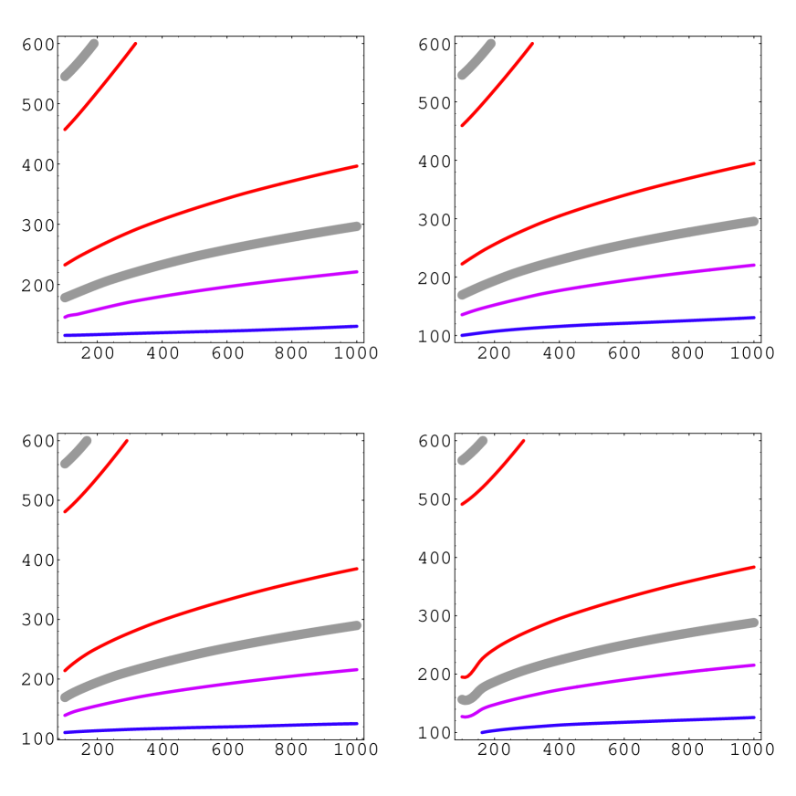
Figure 2: Contour plots of the proton life time in $m_{0}-M_{1/2}$ plane for $\mu<0$ cases. SUSY threshold corrections are calculated using mSUGRA sparticle spectrum with universal boundary conditions $m_{0}$, $M_{1/2}$, $A_{0}$ at the GUT scale. As for $({\rm{tan}}\beta,\;A_{0}[\mbox{GeV}])$, we take them to be $(10,0)$, $(10,-300)$, $(30,0)$, $(30,-300)$, respectively as you can see from each figure. Solid lines correspond to the contours of the proton life time, $5\times 10^{34}$yr., $7\times 10^{34}$yr., $10^{35}$yr., $2\times 10^{35}$yr. from in to out, respectively. Some of them are explicitly denoted in each figure.

We plot the contours of the life time of proton in $m_{0}-M_{1/2}$ plane, where $m_{0}$ and $M_{1/2}$ are the universal soft scalar mass and gaugino mass at the GUT scale, respectively. In Fig.2, we show contours of the proton life time for $\mu<0$ cases with several choices of $A_{0}\;(=0,\;-300{\rm GeV})$, the universal A-term at the GUT scale, and ${\rm{tan}}\beta\;(=10,\;30)$. The contour plots for $\mu>0$ cases are given in Fig. 3.

As we can see from these contours, the proton life time is in the range $3\times 10^{34}-10^{35}$ yr. in most part of the parameter space regardless of choices of ${\rm{tan}}\beta,\;A_{0}$ and sign of $\mu$. We find the minimum of the proton life time is no less than $3\times 10^{34}$ yr. in whole parameter space, which is well above the current experimental limit by the Super-Kamiokande, $5.0\times 10^{33}$ yr. (90% C.L.)[13, 22]. The thick gray contour lines corresponding to the life time of proton $7\times 10^{34}$ yr. represent the $3\sigma$ discovery limit of the $1{\rm{Mt}}$ (fiducial volume) detector after ten years running [12, 13].

Therefore, in the semi-simple unification model, we have an intriguing possibility to confirm the existence of the GUT in nature by observing the proton decay in the next-generation ${\rm{Mt}}$ water $\check{\rm{C}}$erenkov detectors, such as Hyper-Kamiokande [12] and TITAND [13]. In the optimistic cases with some enhancement factors of the decay rate of proton (see below), we have a chance to detect the proton decay also in UNO [23] ($\sim 500{\rm{kt}}$ fiducial volume) experiment.

Although we set the cut-off scale $\Lambda$ to be $10^{17}{\rm GeV}$ in calculating the GUT gauge boson mass to obtain the conservative lower bound of the proton decay rate, the actual cut-off scale may be a little more higher. In that case, the rate is enhanced by $(\Lambda/10^{17}{\rm GeV})^{2}$. Another possible enhancement of the decay rate arises when there are $\mathop{\rm SU}(5)_{\rm GUT}$-charged particles at an intermediate scale. Existence of such particles are highly motivated in the semi-simple unification model; ${\bf 5}+{\bf 5}^{*}$ representations are required at the TeV scale when the discrete ${\bf Z}_{4}$ R symmetry is gauged since the discrete gauge anomaly ${\bf Z}_{4\rm R}$-[$\mathop{\rm SU}(5)_{\rm GUT}$]² should be canceled [24]. In this case, the gauge coupling constant $\alpha_{\rm GUT}$ is stronger as a result of the RG flow with new particles, and the decay rate is enhanced by $1.6$. Although one might suspect that there is a one-loop threshold correction from a possible mass splitting between triplets and doublets in ${\bf 5}+{\bf 5}^{*}$, and that the GUT gauge boson mass would be also changed, the GUT gauge boson mass is actually stable against this correction, since Eq.(13) is an expression from which the threshold corrections from the colored Higgs multiplets decouple. The same thing happens when the SUSY breaking is mediated through gauge mediation because of the presence of the messenger sector, though the SUSY threshold correction should be re-analyzed using the spectrum of the gauge mediated SUSY breaking in that case.

Finally, we summarize various uncertainties in the theoretical prediction given above. The first uncertainty comes from possible violation of the $\mathop{\rm U}(3)_{\rm H}$ relation. The violation $|(1/\alpha_{\rm 3H}-1/\alpha_{\rm 1H})(\Lambda)|=1/3$ leads to a change in the decay rate by $\times/\div 0.5$. The second uncertainty comes from an error bar of the experimental values of the QCD coupling. This results in uncertainties by factor $\times/\div 0.7$ for 1$\sigma$ error. The calculation of hadron matrix element in [16] has an error $W=-0.153(19){\rm GeV}^{2}$, which leads to a factor $\times/\div 0.8$. Another uncertainty comes from a possible non-renormalization operators involving the $\left\langle{\bar{Q}Q}\right\rangle$ vacuum expectation value in the gauge kinetic function of the $\mathop{\rm SU}(5)_{\rm GUT}$ . They generically modifies the $\mathop{\rm SU}(5)_{\rm GUT}$ relation directly by $\left\langle{\bar{Q}Q}\right\rangle/\Lambda^{2}\simeq 10^{-2}$ at tree level. If it is the case, the possible change in the result will be at most roughly the same amount as those discussed above.

There are two more sources of uncertainties whose effects we cannot estimate. First, if one considers an exotic situation in which unknown non-renormalizable operators are relevant in the Wilsonian RG equations, then the perturbative analysis we adopted in this letter is not adequate since we omitted such effects. Secondly, we cannot estimate anything without the ${\cal N}=2$-SUSY relation. This is because the perturbative analysis above the GUT scale is no longer valid without this relation, as is discussed in the appendix.

Appendix A Role of approximate ${\cal N}=2$ SUSY relation
in perturbative analysis

The GUT-breaking sector of the semi-simple unification model has a multiplet structure of ${\cal N}=2$ SUSY, and the interactions between them (the first - the third lines in Eq.(S0.Ex4)) are quite similar to the ${\cal N}=2$ gauge interactions with Fayet-Iliopoulos F-term. Therefore, it is quite likely that this apparent ${\cal N}=2$ structure is a remnant of the ${\cal N}=2$ SUSY in a fundamental theory[15]. Then, the approximate ${\cal N}=2$ relation Eq.(11) at the cut-off scale would be a natural consequence.

The approximate ${\cal N}=2$-relation is not only expected as above, but also almost required from another reason. The perturbation analysis performed in the text is no longer valid if it is not satisfied and that is the reason why we assumed this relation throughout this paper.

Let us suppose that the couplings $\lambda^{(^{\prime})}_{\rm 3H}$ and $\lambda^{(^{\prime})}_{\rm 1H}$ in the superpotential (S0.Ex4) are large compared with $g_{\rm 3H}$ and $g_{\rm 1H}$. Then, those couplings become large extremely fast through one-loop RG equations, and hence we have to require that $\alpha^{\lambda}_{\rm 3H}\equiv\lambda_{\rm 3H}^{2}/(4\pi)$ and $\alpha^{\lambda}_{\rm 1H}\equiv\lambda_{\rm 1H}^{2}/(4\pi)$ are well below $2\alpha_{\rm 3H}$ and $2\alpha_{\rm 1H}$, respectively. The same discussion also holds for $\lambda^{\prime}_{\rm 3H}$ and $\lambda^{\prime}_{\rm 1H}$. Now what if those couplings are small compared with the corresponding gauge couplings? In this case, we can neglect the last two terms in the following two-loop RG equations of the gauge couplings,

$$\frac{\partial}{\partial\ln\mu}\left(\frac{1}{\alpha_{\rm 3H}}\right) \simeq \qquad-\frac{\alpha_{\rm 1H}+17\alpha_{\rm 3H}}{2\pi^{2}}+\frac{\frac{5}{6}(\alpha^{\lambda}_{\rm 1H}+17\alpha^{\lambda}_{\rm 3H})}{2\pi^{2}}+\frac{\frac{1}{6}(\alpha^{\lambda^{\prime}}_{\rm 1H}+17\alpha^{\lambda^{\prime}}_{\rm 3H})}{2\pi^{2}},$$ (24)

$$\frac{\partial}{\partial\ln\mu}\left(\frac{1}{\alpha_{\rm 1H}}\right) \simeq -\frac{6}{2\pi}-\frac{\alpha_{\rm 1H}+8\alpha_{\rm 3H}}{2\pi^{2}}+\frac{\frac{5}{6}(\alpha^{\lambda}_{\rm 1H}+8\alpha^{\lambda}_{\rm 3H})}{2\pi^{2}}+\frac{\frac{1}{6}(\alpha^{\lambda^{\prime}}_{\rm 1H}+8\alpha^{\lambda^{\prime}}_{\rm 3H})}{2\pi^{2}}.$$ (25)

Then, $\alpha_{\rm 3H}$ becomes large quite rapidly and $\alpha_{\rm 1H}$ becomes large more faster than in the one-loop running. Thus, we require that $\alpha^{\lambda^{(^{\prime})}}_{\rm 3H}$ and $\alpha_{\rm 1H}^{\lambda^{(^{\prime})}}$ are comparable to the gauge couplings so that the two-loop effects are negligible.

In the approximate ${\cal N}=2$-SUSY limit and only in this limit, $\alpha_{\rm 3H}\simeq\alpha_{\rm 3H}^{\lambda^{(^{\prime})}}$ and $\alpha_{\rm 1H}\simeq\alpha_{\rm 1H}^{\lambda^{(^{\prime})}}$, anomalous dimensions of hyper multiplets,

$$\gamma_{Q_{i}}=\frac{8\alpha^{\lambda}_{\rm 3H}+\alpha^{\lambda}_{\rm 1H}}{6\pi}-\frac{8\alpha_{\rm 3H}+\alpha_{\rm 1H}}{6\pi}+\cdots,\\$$ (26)

vanish at all order, and the RG flows of the gauge couplings are one-loop exact. Then, in turn, all other parameters in the superpotential, in particular $h$ and $h^{\prime}$, are stable against quantum corrections from the strong couplings $\alpha_{\rm 1H}$, $\alpha_{\rm 3H}$, $\alpha_{\rm 1H}^{\lambda^{(^{\prime})}}$ and $\alpha_{\rm 3H}^{\lambda^{(^{\prime})}}$.

Values of the coupling constants $h$ and $h^{\prime}$ themselves are the possible obstruction left behind for the perturbative analysis. They are obtained from a ratio $\sqrt{M_{c}M_{\bar{c}}}/M_{v}$, which in turn is obtained from Eqs.(S0.Ex5-10) in the way described in the text:

$$\sqrt{hh^{\prime}}=\sqrt{2}g_{\rm GUT}e^{\frac{\pi}{\alpha_{\rm 3H}}(\Lambda)}\left(\frac{\Lambda}{\mu}\right)\exp\left(\frac{2\pi}{12}\left(-\frac{4}{\alpha_{3}}+\frac{9}{\alpha_{2}}-\frac{5}{\alpha_{1}}\right)(\mu)\right)\left(\frac{M_{8v}}{M_{8c}}\right)^{2}e^{\left(\frac{2\pi}{6}\left(\frac{1}{\alpha_{\rm 1H}}-\frac{1}{\alpha_{\rm 3H}}\right)(\Lambda)\right)}.$$ (27)

The value of the RHS of this equation varies from sub-${\cal O}$(1) to ${\cal O}$(1). Therefore, we can expect that the perturbative analysis performed in the text is valid for most part of the SUSY breaking parameter space, taking into account the uncertainties in the gauge coupling constants.

Fields	${\bf 5}^{*}$,${\bf 10}$,${\bf 1}$	$H$ , $\bar{H}$	$X^{\alpha}_{\;\beta}$	$Q_{i}$,$\bar{Q}^{i}$	$Q_{6}$	$\bar{Q}^{6}$
${\bf Z}_{4}$ R charge	1	0	2	0	2	-2

Table 1: Charge assignment of the ${\bf Z}_{4}$ R-symmetry is given. ${\bf 1}$ denotes a right handed neutrino.

(${\bf 3},{\bf 2})^{-\frac{5}{6}}$	$({\bf 3},{\bf 1})^{-\frac{1}{3}}$	$({\bf 3},{\bf 1})^{-\frac{1}{3}}$	$({\bf 1},{\bf 1})^{0}$	$({\bf 1},{\bf 1})^{0}$	$({\bf adj.},{\bf 1})^{0}$	$({\bf adj.},{\bf 1})^{0}$
m.vect.	$\chi+\chi^{\dagger}$	$\chi+\chi^{\dagger}$	m.vect.	$\chi+\chi^{\dagger}$	m.vect.	$\chi+\chi^{\dagger}$
$M_{v}=$	$M_{c}=$	$M_{\bar{c}}=$	$M_{1v}=$	$M_{1c}=$	$M_{8v}=$	$M_{8c}=$
$\sqrt{2}g_{\rm GUT}v$	$hv$	$h^{\prime}v$	$\sqrt{2(g_{\rm 1H}^{2}+2g_{\rm GUT}^{2}/5)}v$	$\sqrt{2}\lambda_{\rm 1H}v$	$\sqrt{2(g_{\rm 3H}^{2}+g_{\rm GUT}^{2})}v$	$\sqrt{2}\lambda_{3H}v$

Table 2: Summary of the particle spectrum around the GUT scale. The first line denotes the representation under the MSSM gauge group. In the second line, m.vect. denotes ${\cal N}=1$ massive vector multiplet and $\chi+\chi^{\dagger}$ a pair of ${\cal N}=1$ chiral and anti-chiral multiplet. Mass of each multiplet is given in terms of gauge couplings and parameters in the superpotential (S0.Ex4) in the fourth line, and given in the third line is the expression of the mass used in the text. Multiplets with masses $M_{1v}$ and $M_{1c}$, $M_{8v}$ and $M_{8c}$ can be regarded as ${\cal N}=2$-SUSY partner with each other in the ${\cal N}=2$-SUSY limit(see also appendix).

Figure 3: Contour plots of the proton life time in $m_{0}-M_{1/2}$ plane for $\mu>0$ cases. Other conventions are the same as those in Fig. 2.

References

[1]
P. Langacker and M. Luo,
Phys. Rev. D 44 (1991) 817.
[2]
H. Georgi and S. L. Glashow,
Phys. Rev. Lett. 32 (1974) 438.
[3]
N. Sakai and T. Yanagida,
Nucl. Phys. B 197 (1982) 533;
S. Weinberg,
Phys. Rev. D 26 (1982) 287.
[4]
J. Hisano, T. Moroi, K. Tobe and T. Yanagida,
Mod. Phys. Lett. A 10 (1995) 2267
[arXiv:hep-ph/9411298].
H. Murayama and A. Pierce,
arXiv:hep-ph/0108104.
[5]
Y. Hayato et al. [SuperKamiokande Collaboration],
Phys. Rev. Lett. 83 (1999)1529
[arXiv:hep-ex/9904020].
[6]
E. Witten,
Nucl. Phys. B 258 (1985) 75.
[7]
L. Maiani, in Comptes Rendus de l’Ecole d’Et de
Physique des Particules, Gif-sur-Yvette,1979;
S. Dimopoulos and H.Georgi, Nucl. Phys. B150 (1981) 193;
M. Sakai, Z. Phys. C11 (1981) 153;
E. Witten, Nucl. Phys. B188 (1981) 573.
[8]
T. Yanagida,
Phys. Lett. B 344 (1995) 211
[hep-ph/9409329].
[9]
J. Hisano and T. Yanagida,
Mod. Phys. Lett. A 10 (1995) 3097
[hep-ph/9510277];
T. Hotta, K. I. Izawa and T. Yanagida,
Phys. Rev. D 53 (1996) 3913
[hep-ph/9509201],
T. Hotta, K. I. Izawa and T. Yanagida,
Phys. Rev. D 54 (1996) 6970
[hep-ph/9602439].
[10]
K. I. Izawa and T. Yanagida,
Prog. Theor. Phys. 97 (1997) 913
[hep-ph/9703350].
[11]
J. Hisano, H. Murayama and T. Yanagida,
Nucl. Phys. B 402 (1993) 46
[arXiv:hep-ph/9207279].
[12]
M. Koshiba, Phys. Rep.220, 229 (1992);
K. Nakamura, talk presented at Int. Workshop on Next Generation Nucleon
Decay and Neutrino Detector, 1999, SUNY at Stony Brook;
K. Nakamura, Neutrino Oscillation and Their Origin,
(Universal Academy Press, Tokyo, 2000), p. 359.
[13]
Y. Suzuki et al. [TITAND Working Group Collaboration],
arXiv:hep-ex/0110005.
[14]
G. F. Giudice and A. Masiero,
Phys. Lett. B 206 (1988) 480.
[15]
Y. Imamura, T. Watari and T. Yanagida,
Phys. Rev. D 64 (2001) 065023
[arXiv:hep-ph/0103251];
T. Watari and T. Yanagida,
Phys. Lett. B 520 (2001) 322
[arXiv:hep-ph/0108057].
[16]
S. Aoki et al., Phys. Rev. D62, 014506 (2000).
[17]
D. M. Pierce, J. A. Bagger, K. T. Matchev and R. j. Zhang,
Nucl. Phys. B 491 (1997) 3
[arXiv:hep-ph/9606211].
[18]
S. Fanchiotti, B. Kniehl and A. Sirlin,
Phys. Rev. D 48 (1993) 307 [arXiv:hep-ph/9212285].
[19]
S. Eidelman and F. Jegerlehner,
Z. Phys. C 67 (1995) 585
[arXiv:hep-ph/9502298].
[20]
Particle data group.D. E. Groom et al. [Particle Data Group Collaboration],
Eur. Phys. J. C 15 (2000) 1.
[21]
B. C. Allanach,
arXiv:hep-ph/0104145.
[22]
M. Shiozawa et al. [Super-Kamiokande Collaboration],
Phys. Rev. Lett. 81 (1998) 3319
[arXiv:hep-ex/9806014].
[23]
C. K. Jung,
arXiv:hep-ex/0005046.
[24]
K. Kurosawa, N. Maru and T. Yanagida,
Phys. Lett. B 512 (2001) 203
[arXiv:hep-ph/0105136].