Longitudinal Polarization Asymmetry of Leptons
in pure Leptonic $B$ Decays

Abstract

Longitudinal polarization asymmetry of leptons in $B_{q}\rightarrow\ell^{+}\,\ell^{-}$ ($q=d,s$ and $\ell=e,\mu,\tau$) decays is investigated. The analysis is done in a general manner by using the effective operators approach. It is shown that the longitudinal polarization asymmetry would provide a direct search for the scalar and pseudoscalar type interactions, which are induced in all variants of Higgs-doublet models.

It has been already pointed out by several authors [1, 2, 3, 4] that the pure leptonic $B$ decays $B_{q}\rightarrow\ell^{+}\,\ell^{-}$ ($q=d,s$ and $\ell=e,\mu,\tau$) are very good probes to test new physics beyond the standard model (SM), mainly to reveal the Higgs sector. Those previous works were focused on the contributions induced by the scalar and pseudoscalar interactions realized in Higgs-doublets models. Within the SM, the decays are dominated by the $Z-$penguin and the box diagrams, which are helicity suppressed. We note that Higgs-doublet models can generally enhance the branching ratio significantly. Also, as discussed in recent works, the decays are strongly correlated with the semi-leptonic $B$ decays [4] and even with the muon anomalous magnetic moment [5]. Experimentally, it is expected that present and the forthcoming experiments on the $B-$physics ($B-$factories) can probe the flavor sector with high precision [6].

If we detect large discrepancy between the theoretical estimation of the decay branching fractions and the actually observed experimental results, then this could be either an evidence of new physics or of our lack of knowledge of the decay constants of $B$ mesons, $f_{B_{q}}$. Therefore, the main interest would be a direct observation of new physics contributions belonging to the non-SM interactions, $i.e.$ the scalar and pseudoscalar interactions, because within the SM the decay is only through the axial vector interactions. In this letter, we propose a new observable, namely the longitudinal polarization asymmetry of leptons (${\cal A}_{\rm LP}$) in $B_{q}\rightarrow\ell^{+}\,\ell^{-}$ ($q=d,s$ and $\ell=e,\mu,\tau$) decays. Though the measurement may be very difficult and challenging, we point out that this observable is very sensitive to those non-SM new interactions, and provides a direct evidence of their existence. We notice that the idea of measuring ${\cal A}_{\rm LP}$ and CP–violation in $K_{L}\rightarrow\mu^{+}\,\mu^{-}$ decay to look for new physics has been previously considered in several papers [7]. However, we would like to mention that those observables are quite different in the $B$ decay system [8, 9]: In the $K$ system the initial CP–eigenstate can be determined due to large lifetime difference of $K_{L,S}$, while such determination is not possible in the case of $B$ meson system. Therefore, we cannot discuss the $B_{q}\rightarrow\ell^{+}\,\ell^{-}$ decays in the same manner as those previous references.

Taking into account all possible 4-fermi operators which could contribute to $B_{q}\rightarrow\ell^{+}\,\ell^{-}$, these processes are governed by the following effective Hamiltonian [10],

$${\cal H}_{\rm eff} = -\frac{G_{F}\alpha}{2\sqrt{2}\pi}\left(V_{tq}^{\ast}V_{tb}\right)\,\left\{{\cal C}_{\rm AA}(\bar{q}\,\gamma_{\mu}\gamma_{5}\,b)(\bar{\ell}\,\gamma^{\mu}\gamma_{5}\,\ell)\right.$$ (1)

$$\left.\;\;\;\;\;\;\;\;\;\;\;\;\;\;+{\cal C}_{\rm PS}(\bar{q}\,\gamma_{5}\,b)(\bar{\ell}\,\ell)+{\cal C}_{\rm PP}(\bar{q}\,\gamma_{5}\,b)(\bar{\ell}\,\gamma_{5}\,\ell)\right\}\;,$$

by normalizing all terms with the overall factors of the SM. In particular, within the SM one has ${\cal C}_{\rm PS}^{\rm SM}={\cal C}_{\rm PP}^{\rm SM}\simeq 0$ and ${\cal C}_{\rm AA}^{\rm SM}={Y(x_{t_{W}})}/{\sin^{2}\theta_{W}}$, where $Y(x_{t_{W}})$ is the Inami-Lim function [11] with $x_{t_{W}}=({m_{t}}/{M_{W}})^{2}$. The contributions proportional to $m_{d,s}$ are neglected, and the neutral Higgs contributions in ${\cal C}_{\rm PS}^{\rm SM}$ and ${\cal C}_{\rm PP}^{\rm SM}$ are proportional to ${(m_{\ell}m_{b})}/{m_{W}}^{2}$, and therefore also neglected.

After using the PCAC ansatz to derive the relation between the operators, the most general matrix element for the decay is

$${\cal M} = if_{B_{q}}\frac{G_{F}\alpha}{2\sqrt{2}\pi}V_{tq}^{*}V_{tb}\left[\left(2m_{\ell}{\cal C}_{\rm AA}-\frac{m_{B_{q}}^{2}}{m_{b}+m_{q}}{\cal C}_{\rm PP}\right)\bar{\ell}\,\gamma_{5}\,\ell-\frac{m_{B_{q}}^{2}}{m_{b}+m_{q}}{\cal C}_{\rm PS}\bar{\ell}\,\ell\right].$$ (2)

Using Eq. (2), the branching ratio for $B_{q}\rightarrow\ell^{+}\,\ell^{-}$ becomes

$${\cal B}(B_{q}\rightarrow\ell^{+}\,\ell^{-}) = \frac{G_{F}^{2}\,\alpha^{2}}{64\pi^{3}}\,\left|V_{tq}^{\ast}V_{tb}\right|^{2}\,\tau_{B_{q}}f_{B_{q}}^{2}\,m_{B_{q}}\,\sqrt{1-\frac{4m_{\ell}^{2}}{m_{B_{q}}^{2}}}$$ (3)

$$\times\left[\left|2m_{\ell}~{}{\cal C}_{\rm AA}-\frac{m_{B_{q}}^{2}}{m_{b}+m_{q}}{\cal C}_{\rm PP}\right|^{2}+\left(1-\frac{4m_{\ell}^{2}}{m_{B_{q}}^{2}}\right)\left|\frac{m_{B_{q}}^{2}}{m_{b}+m_{q}}{\cal C}_{\rm PS}\right|^{2}\right],$$

where $\tau_{B_{q}}$ is the life-time of $B_{q}$ meson. The QCD correction in this decay mode is remarkably negligible. As can be easily seen, the significant branching ratio within the SM could be expected only for $\ell=\tau,\mu$ due to the lepton mass dependence.

We now define an observable using the lepton polarization. Since in the dilepton rest frame we can define only one direction, the lepton polarization vectors in each lepton’s rest frame are defined as

$$\bar{s}^{\mu}_{\ell^{\pm}}=\left(0,\pm\frac{\mathbf{\rm p_{-}}}{|\mathbf{\rm p_{-}}|}\right)\;,$$ (4)

and in the dilepton rest frame they are boosted to

$$s^{\mu}_{\ell^{\pm}}=\left(\frac{|\mathbf{\rm p_{-}}|}{m_{\ell}},\pm\frac{E_{\ell}\mathbf{\rm p_{-}}}{m_{\ell}|\mathbf{\rm p_{-}}|}\right)\;,$$ (5)

where $E_{\ell}$ is the lepton energy. Finally the longitudinal polarization asymmetry of the final leptons in $B_{q}\rightarrow\ell^{+}\,\ell^{-}$ is defined as follows;

$${\cal A}_{\rm LP}^{\pm}\equiv\frac{\left[\Gamma(s_{\ell^{-}},s_{\ell^{+}})+\Gamma(\mp s_{\ell^{-}},\pm s_{\ell^{+}})\right]-\left[\Gamma(\pm s_{\ell^{-}},\mp s_{\ell^{+}})+\Gamma(-s_{\ell^{-}},-s_{\ell^{+}})\right]}{\left[\Gamma(s_{\ell^{-}},s_{\ell^{+}})+\Gamma(\mp s_{\ell^{-}},\pm s_{\ell^{+}})\right]+\left[\Gamma(\pm s_{\ell^{-}},\mp s_{\ell^{+}})+\Gamma(-s_{\ell^{-}},-s_{\ell^{+}})\right]}\;,$$ (6)

and it becomes

$${\cal A}_{\rm LP}(B_{q}\rightarrow\ell^{+}\,\ell^{-}) = \frac{2\sqrt{1-\frac{4m_{\ell}^{2}}{m_{B_{q}}^{2}}}Re\left[\frac{m_{B_{q}}^{2}}{m_{b}+m_{q}}{\cal C}_{\rm PS}\left(2m_{\ell}{\cal C}_{\rm AA}-\frac{m_{B_{q}}^{2}}{m_{b}+m_{q}}~{}{\cal C}_{\rm PP}\right)\right]}{\left|2m_{\ell}{\cal C}_{\rm AA}-\frac{m_{B}^{2}}{m_{b}+m_{q}}{\cal C}_{\rm PP}\right|^{2}+(1-\frac{4m_{\ell}^{2}}{m_{B_{q}}^{2}})\left|\frac{m_{B_{q}}^{2}}{m_{b}+m_{q}}{\cal C}_{\rm PS}\right|^{2}},$$ (7)

with ${\cal A}_{\rm LP}^{+}={\cal A}_{\rm LP}^{-}\equiv{\cal A}_{\rm LP}$. It is clear that within the SM ${\cal A}_{\rm LP}(B_{q}\rightarrow\ell^{+}\,\ell^{-})\simeq 0$, and becomes non-zero if and only if ${\cal C}_{\rm PS}\neq 0$. Therefore, this observable would be the best probe to search for new physics induced by the pseudoscalar type interactions. We also remark that the dependence on the flavor of the valence quark in ${\cal A}_{\rm LP}(B_{q}\rightarrow\ell^{+}\,\ell^{-})$ is tiny, therefore the lepton longitudinal polarization asymmetry is almost the same for $q=d$ or $q=s$.

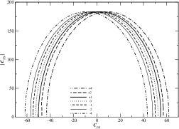
Figure 1: The upper bounds for ${\cal C}_{\rm PP}$ vs $|{\cal C}_{\rm PS}|$ for ${\cal C}_{\rm AA}=(-4,-2,-1,0,+1,+2,+4)\times{\cal C}_{\rm AA}^{\rm SM}$ using the experimental bound on ${\cal B}(B_{s}\rightarrow\mu^{+}\,\mu^{-})$ (left); and the indirect experimental bound on ${\cal B}(B_{s}\rightarrow\tau^{+}\,\tau^{-})$ (right).

Before considering physics beyond the SM, let us briefly review the SM predictions for the processes. For consistency, the top mass is rescaled from its pole mass, $m_{t}=175\pm 5$ GeV, to the $\overline{\rm MS}-$mass, $m_{t}(\overline{\rm MS})=167\pm 5$ GeV. For numerical calculations throughout the paper, we use the world–averaged values for all other parameters [12], i.e. :

$m_{B_{q}^{0}}=5279.2\pm 1.8$ MeV, $m_{W}=80.41\pm 0.10$ GeV, $\tau_{B_{q}^{0}}=1.56\pm 0.04$ (ps)^-1, $m_{e}=0.5$ MeV, $m_{\mu}=105.7$ MeV, $m_{\tau}=1777$ MeV, $\sin^{2}\theta_{W}(\overline{\rm MS})=0.231$, $\alpha=1/{129}$, $f_{B_{d}}=210\pm 30$ MeV and $f_{B_{s}}=245\pm 30$ MeV [13].

Within the SM and by using the experimental bounds on the Wolfenstein parametrization $(A,\lambda)=(0.819\pm 0.035,0.2196\pm 0.0023)$ together with the unitarity of CKM matrix [12, 14], we get

$$\begin{array}[]{rcl}|V_{ts}|&\approx&A\,\lambda^{2}=0.0395\pm 0.0019\,,\\ |V_{td}|&\approx&A\,\lambda^{3}\sqrt{(1-\rho)^{2}+\eta^{2}}=0.004\sim 0.013\,.\end{array}$$ (8)

Adopting the next-to-leading order result for $Y(x_{t_{W}})$ [15], and using the central values for all input parameters, lead to the following SM predictions,

$${\cal B}(B_{d}\rightarrow\ell^{+}\,\ell^{-}) = \left\{\begin{array}[]{lcl}3.4\times{10}^{-15}\left(\frac{f_{B_{d}}}{210~{}MeV}\right)^{2}&,&\ell=e\\ 1.5\times{10}^{-10}\left(\frac{f_{B_{d}}}{210~{}MeV}\right)^{2}&,&\ell=\mu\\ 3.2\times{10}^{-8}\left(\frac{f_{B_{d}}}{210~{}MeV}\right)^{2}&,&\ell=\tau\end{array}\right.\,,$$ (12)

$${\cal B}(B_{s}\rightarrow\ell^{+}\,\ell^{-}) = \left\{\begin{array}[]{lcl}8.9\times{10}^{-14}\left(\frac{f_{B_{s}}}{245~{}MeV}\right)^{2}&,&\ell=e\\ 4.0\times{10}^{-9}\left(\frac{f_{B_{s}}}{245~{}MeV}\right)^{2}&,&\ell=\mu\\ 8.3\times{10}^{-7}\left(\frac{f_{B_{s}}}{245~{}MeV}\right)^{2}&,&\ell=\tau\end{array}\right.\,.$$ (16)

These predictions should be confronted with the present experimentally known bounds of ${\cal B}(B_{q}\rightarrow\ell^{+}\,\ell^{-})$ at $95\%$ CL [16],

$${\cal B}(B_{d}\rightarrow\mu^{+}\,\mu^{-}) < 8.6\times{10}^{-7}\,,$$ (17)

$${\cal B}(B_{s}\rightarrow\mu^{+}\,\mu^{-}) < 2.6\times{10}^{-6}\,.$$ (18)

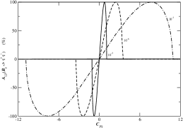
Figure 2: The correlation between ${\cal A}_{\rm LP}(B_{s}\rightarrow\tau^{+}\,\tau^{-})$ and ${\cal C}_{\rm PS}$ for various ${\cal B}(B_{s}\rightarrow\tau^{+}\,\tau^{-})=10^{-5},10^{-6},10^{-7}$ (left); and the correlation between ${\cal A}_{\rm LP}(B_{s}\rightarrow\tau^{+}\,\tau^{-})$ and ${\cal B}(B_{s}\rightarrow\tau^{+}\,\tau^{-})$ for various ${\cal C}_{\rm PS}=1.6,5.0,10.2,17.3,26.2$ (right).

To analyze the decay processes and simulataneously find the possible new physics signal, we first employ the experimental bound of the branching ratio which constraints the coefficients (${\cal C}$’s) more strictly after comparing the theoretical predictions with the known experimental bounds, $i.e.$ ${\cal B}(B_{s}\rightarrow\mu^{+}\,\mu^{-})$ (see Eqs. (12)$\sim$(18)), and obtain the allowed region on the ${\cal C}_{\rm PS}-{\cal C}_{\rm PP}$ parameter space for various values of ${\cal C}_{\rm AA}$. This is shown in the left-hand-side figure of Fig. 1. In the right-hand-side figure the bound is obtained by using the indirect experimental bound ${\cal B}(B_{s}\rightarrow\tau^{+}\,\tau^{-})<4.3\times 10^{-4}$ [17]. Furthermore, suppose that the branching ratio is measured first, then it must be worth to show a general correlation between the branching ratio and the longitudinal polarization asymmetry represented by the following equation,

$${\cal A}_{\rm LP}(B_{q}\rightarrow\ell^{+}\,\ell^{-}) = \pm\frac{2a_{q}\sqrt{1-\frac{4m_{\ell}^{2}}{m_{B_{q}}^{2}}}}{{\cal B}(B_{q}\rightarrow\ell^{+}\,\ell^{-})}\,Re\left[\frac{m_{B_{q}}^{2}}{m_{b}+m_{q}}{\cal C}_{\rm PS}\right.$$ (19)

$$\left.\times\sqrt{\frac{{\cal B}(B_{q}\rightarrow\ell^{+}\,\ell^{-})}{a_{q}}-\left(1-\frac{4m_{\ell}^{2}}{m_{B_{q}}^{2}}\right)\left|\frac{m_{B_{q}}^{2}}{m_{b}+m_{q}}{\cal C}_{\rm PS}\right|^{2}}\right]\,,$$

by eliminating ${\cal C}_{\rm AA}$ and ${\cal C}_{\rm PP}$ in Eqs. (3) and (7), where the constant $a_{q}$ is defined as

$$a_{q}\equiv\frac{G_{F}^{2}\alpha^{2}}{64\pi^{3}}\,\left|V_{tq}^{\ast}V_{tb}\,\right|^{2}\tau_{B_{q}}f_{B_{q}}^{2}m_{B_{q}}\,\sqrt{1-\frac{4m_{\ell}^{2}}{m_{B_{q}}^{2}}}\,.$$ (20)

This is depicted in Fig. 2. The left-hand-side figure shows a correlation between ${\cal A}_{\rm LP}(B_{s}\rightarrow\tau^{+}\,\tau^{-})$ and ${\cal C}_{\rm PS}$ for various ${\cal B}(B_{s}\rightarrow\tau^{+}\,\tau^{-})$, while the right-hand-side one is between ${\cal A}_{\rm LP}(B_{s}\rightarrow\tau^{+}\,\tau^{-})$ and ${\cal B}(B_{s}\rightarrow\tau^{+}\,\tau^{-})$ for various ${\cal C}_{\rm PS}$.

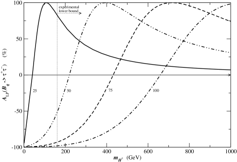
Figure 3: The longitudinal polarization asymmetry of $\tau$’s, ${\cal A}_{\rm LP}(B_{q}\rightarrow\tau^{+}\,\tau^{-})$, as a function of $m_{H^{\pm}}$ for various $\tan\beta=25,50,75,100$.

As a specific example for the case in which ${\cal C}_{\rm PS}$ is non-zero, we adopt the type II 2-Higgs-doublet models (2HDM-II). In this model

$${\cal C}_{\rm AA}^{\rm 2HDM-II}={\cal C}_{\rm AA}^{\rm SM},$$

while

$${\cal C}_{\rm PS}^{\rm 2HDM-II}={\cal C}_{\rm PP}^{\rm 2HDM-II}=\frac{m_{\ell}(m_{b}+m_{q})}{4M_{W}^{2}\sin^{2}\theta_{W}}\,\tan^{2}\beta\frac{\ln x_{H^{\pm}t}}{x_{H^{\pm}t}-1}\;,$$ (21)

at large $\tan\beta$ limit [2, 3, 4], and $x_{H^{\pm}t}=({m_{H^{\pm}}}/{m_{t}})^{2}$. Some particular cases in the right-hand-side figure of Fig. 2 can be realized by, for instance,

$(m_{H^{\pm}},\tan\beta)=(200\,{\rm GeV},40)$ for ${\cal C}_{\rm PS}=1.6$, $(200\,{\rm GeV},70)$ for ${\cal C}_{\rm PS}=5.0$, $(200\,{\rm GeV},100)$ for ${\cal C}_{\rm PS}=10.2$, $(200\,{\rm GeV},130)$ for ${\cal C}_{\rm PS}=17.3$, $(200\,{\rm GeV},160)$ for ${\cal C}_{\rm PS}=26.2$.

Finally, in Fig. 3 we show the dependences of ${\cal A}_{\rm LP}(B_{q}\rightarrow\tau^{+}\,\tau^{-})$ on $m_{H^{\pm}}$ and $\tan\beta$. For the real experimental analyses, we recommend $B_{s}\rightarrow\tau^{+}\,\tau^{-}$ decays because the energy of final $\tau$’s is high enough to decay further to energetic secondary particles, so their longitudinal polarization may be well measured in hadronic $B-$factories. Although the $\tau$’s are difficult to be reconstructed in hadronic background, we need precisely such reconstruction from their decay products that allows measurements of the longitudinal polarization of $\tau$’s.

In conclusion we have considered a general analysis exploring the longitudinal polarization asymmetry of leptons in the $B_{q}\rightarrow\ell^{+}\,\ell^{-}$ decays. We have shown that this observable would provide a direct measurement of the physics of scalar and pseudoscalar type interactions. We also note that more information about these new interactions can be obtained by combining the present analysis with the other observables from $B\rightarrow X_{q}\ell^{+}\ell^{-}$ [18].

We thank G. Cvetic and D. London for careful reading of the manuscript and their valuable comments. The work of C.S.K. was supported by Grant No. 2001-042-D00022 of the KRF. The work of T.Y. was supported in part by the US Department of Energy under Grant No.DE-FG02-97ER-41036.

References

[1]
K. S. Babu and C. Kolda,
Phys. Rev. Lett.84 (2000) 228.
[2]
H. E. Logan and U. Nierste,
Nucl. Phys.B586 (2000) 39.
[3]
C.-S. Huang, W. Liao, Q.-S. Yan and S.-H. Zhu,
Phys. Rev.D63 (2001) 114021,
[ErrD64 (2001) 059902].
[4]
C. Bobeth, T. Ewerth, F. Krger and J. Urban,
Phys. Rev.D64 (2001) 074014.
[5]
A. Dedes, H. K. Dreiner and U. Nierste,
hep-ph/0108037 (2001).
[6]
D. Boutigny et.al. (BaBar Collaboration),
SLAC-R-0457 (1995) ;
M. T. Cheng et.al. (Belle Collaboration),
BELLE-TDR-3-95 (1995) ;
P. Krizan et.al. (HERA-B Collaboration),
Nucl. Inst. Meth.A351 (1994) 111;
W.W. Armstrong et.al. (ATLAS Collaboration),
CERN/LHCC/94-43 (1994) ;
S. Amato et.al. (LHCb Collaboration),
CERN/LHCC/98-4 (1998) .
[7]
P. Herczeg,
Phys. Rev.D27 (1989) 1512;
F. J. Botella and C. S. Lim,
Phys. Rev. Lett.56 (1986) 1651;
C. Q. Geng and J. N. Ng,
Phys. Rev. Lett.62 (1989) 2645.
[8]
X-G. He, J. P. Ma and B. McKellar,
Phys. Rev.D49 (1994) 4548.
[9]
C.-S. Huang, W. Liao,
hep-ph/0011089.
[10]
Y. Grossman, Z. Ligeti and E. Nardi,
Phys. Rev.D55 (1997) 2768;
D. Guetta and E. Nardi,
Phys. Rev.D58 (1998) 012001.
[11]
T. Inami and C. S. Lim,
Prog. Theor. Phys.65 (1981) 297
[Err.65 (1981) 1772].
[13]
S. Hashimoto,
Nucl. Phys.Proc.Suppl.B83 (2000) 3.
[14]
See for example:
A. Ali and D. London,
Euro. Phys. Jour.C9 (1999) 687.
[15]
G Buchalla and A. J. Buras,
Nucl. Phys.B400 (1993) 225;
M. Misiak and J. Urban,
Phys. Lett.B451 (1999) 161.
[16]
F. Abe et.al. (CDF Collaboration),
Phys. Rev.D57 (1998) R3811.
[17]
G. Isidori and A. Retico,
JHEP2001 (0111:001) .
[18]
S. Fukae, C.S. Kim, T. Morozumi and T. Yoshikawa,
Phys. Rev.D59 (1999) 074013;
S. Fukae, C.S. Kim and T. Yoshikawa,
Phys. Rev.D61 (1999) 074015;
S. Fukae, C.S. Kim and T. Yoshikawa,
Int. Jour. Mod. Phys.A16 (2001) 1703.