TUM-HEP-449/01 Effects of random matter density fluctuations on the neutrino oscillation transition probabilities in the Earth

Abstract

Abstract

In this paper, we investigate the effects of random fluctuations of the Earth matter density for long baselines on the neutrino oscillation transition probabilities. We especially identify relevant parameters characterizing the matter density noise and calculate their effects by averaging over statistical ensembles of a large number of matter density profiles. For energies and baselines appropriate to neutrino factories, absolute errors on the relevant appearance probabilities are at the level of $|\Delta P_{\alpha\beta}|\sim 10^{-4}$ (with perhaps $|\Delta P_{\mu e}|/P_{\mu e}\sim 1\%$ for neutrinos), whereby a modest improvement in understanding of the geophysical data should render such effects unimportant.

PACS: 14.60.Lm, 13.15.+g, 91.35.-x, 23.40.Bw
Key words: Neutrino oscillations, Matter effects, Earth’s matter density profile, Long baseline neutrino experiments

1 Introduction

The effects of matter on neutrino oscillations [1, 2, 3] in the Earth have been investigated in various contexts and with several models [4, 5, 6, 7, 8, 9, 10, 11, 12, 13, 14, 15, 16, 17, 18, 19, 20, 21, 22, 23, 24, 25, 26, 27, 28, 29, 30]. It is now well-known that the matter density can significantly change the reconstructed neutrino energy spectrum produced by long baseline neutrino experiments, such as by neutrino factories [31, 32, 20]. For most calculations the Preliminary Reference Earth Model (PREM) density profile [33] has been used, which is obtained from geophysical seismic wave measurements (see, e.g., Refs. [34, 35, 36] for information about the structure of the Earth’s interior). Furthermore, small errors in the PREM matter density with up to 5% amplitude have been found and documented by many geophysics groups (for a summary, see, e.g., Ref. [37]). Note, however, that the Earth’s matter density distribution is not directly observable from seismological data [38, 39]. In this paper, we will discuss how these fluctuations in the Earth matter density affect the neutrino oscillation transition probabilities.

It has been found that for short baselines matter effects are small [40]. Thus, any fluctuations could be treated as second order effects and can therefore be neglected. For long baselines, however, the fluctuations may be significant. It was noted in Ref. [41] that this effect can be important as an additional uncertainty in the determination of the CP phase $\delta_{CP}$, especially for certain values of $\delta_{CP}$. To estimate this effect, the authors used a logarithmic distribution with a certain length scale and amplitude with a path integral method for the numerical evaluation. On the other hand, it was shown in Ref. [42], using a perturbation theoretical approach, that fluctuations with small amplitudes on length scales much shorter than the oscillation length in matter average out and give no net effect at all. In this paper, we are interested in the errors on the transition probabilities as functions of the length scale and amplitude of the matter density fluctuations. We will, in particular, focus on the errors on the appearance probability of electron neutrinos and electron antineutrinos at typical neutrino factory energies, since matter density noise effects could be rather substantial in the determination of the CP phase and matter effects are largest in the appearance channel.

2 The effect of a matter density perturbation

Before we come to modeling the fluctuations in the Earth matter density profile, let us study the effect of a single perturbation in the matter density. In any quantum mechanical system, described by a Schrödinger equation, the impact on a free particle’s motion of a potential depends on its length scale as well as its amplitude. When the length scale of the potential is much shorter than the characteristic wave length of the incident particle, the particle’s wave function will be unable to resolve the exact spatial structure of this potential. It is then possible to replace the potential by a $\delta$-distribution with an amplitude equal to the integral of the original potential. Similarly, in neutrino oscillations, described by a Schrödinger equation, a perturbation on a length scale much shorter than the oscillation length in matter could be replaced by a $\delta$-distribution.

Figure 1: The plot on the left-hand side shows the relative error $|\Delta P_{\mu e}|/P_{\mu e}^{\mathrm{ref}}$ in the appearance probability of the unperturbed profile $P_{\mu e}^{\mathrm{ref}}$ with a rectangular matter density perturbation of length $\lambda$ and amplitude $\Delta\rho\equiv\rho-\bar{\rho}$, where $\bar{\rho}=3\,\mathrm{g/cm^{3}}$ is the average matter density. The perturbation is assumed to be centered at a baseline of length $L=7400\,\mathrm{km}$. The relative error is plotted as a function of the product of the relative length scale $\lambda/L^{\mathrm{osc}}_{\mathrm{matter}}$ and the relative density contrast $\Delta\rho/\bar{\rho}$. Here $L^{\mathrm{osc}}_{\mathrm{matter}}\simeq 17000\,\mathrm{km}$ is the oscillation length in matter, determined by the average matter density $\bar{\rho}$ and the leading neutrino oscillation parameters $\Delta m_{32}^{2}$ and $\theta_{13}$ for a typical neutrino factory maximum energy chosen to be $E=30\,\mathrm{GeV}$. The plot on the right-hand side shows this density perturbation for a fixed value of the area spanned by the length scale and the amplitude, i.e., $\lambda\,\Delta\rho=0.01\,\bar{\rho}\,L^{\mathrm{osc}}_{\mathrm{matter}}$, which is indicated as a vertical line in the left plot. In both plots, the length scale is fixed to be $5\,\mathrm{km}$ (dotted curves), $500\,\mathrm{km}$ (dashed curves), and $2000\,\mathrm{km}$ (solid curves), respectively.

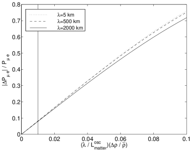
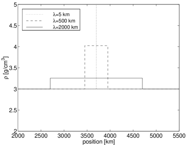
This can be seen in Fig. 1 (left plot), where the relative error $|\Delta P_{\mu e}|/P_{\mu e}^{\mathrm{ref}}\equiv|P_{\mu e}-P_{\mu e}^{\mathrm{ref}}|/P_{\mu e}^{\mathrm{ref}}$, coming from a rectangular matter density perturbation, is plotted as a function of the product of the length scale $\lambda/L^{\mathrm{osc}}_{\mathrm{matter}}$ and the density contrast $\Delta\rho/\bar{\rho}$. For the oscillation parameters we choose $\theta_{12}=45^{\circ}$, $\theta_{23}=45^{\circ}$, $\theta_{13}=5^{\circ}$, $\Delta m_{32}^{2}=2.5\cdot 10^{-3}\,\mathrm{eV}^{2}$, $\Delta m_{21}^{2}=3.65\cdot 10^{-5}\,\mathrm{eV}^{2}$, and $\delta_{CP}=0$, corresponding to the LMA solution with a value for $\theta_{13}$ somewhat below the CHOOZ bound neglecting CP violating effects. The other parameters (and terms) are given and described in the figure caption. The relative error is shown for several fixed values of $\lambda\ll L^{\mathrm{osc}}_{\mathrm{matter}}$, i.e., only the matter density is varied in such a way that the area of the perturbation is unaffected for a fixed value on the horizontal axis. For the cut at the vertical line this constant area of the matter density perturbation is shown in the right plot, indicating that the corresponding parameter value is already a quite pessimistic choice. Apparently, the curves in the left plot are approximately equal to each other at least below the parameter value indicated by the vertical line and especially for very small fixed values of $\lambda$. This means that the relevant parameter for $\lambda\ll L^{\mathrm{osc}}_{\mathrm{matter}}$ is the integral of the matter density perturbation, i.e., the product of the length scale and the amplitude. Thus, we may expect that interference effects, arising from non-commuting operators in the Hamiltonian corresponding to different matter density layers, become irrelevant for very short length scales compared with the oscillation length in matter. This can also be seen in the analytical perturbation theoretical approach in App. A, where the case of baselines much shorter than the oscillation length leads to first order corrections $\propto\lambda\,\Delta\rho$ to the transition probabilities, i.e., the product of the length scale and the amplitude is the relevant parameter. Another result of the numerical analysis is that we do not have to take into account isolated short scale perturbations, such as the ones coming from the matter density contrast in, for example, a mine. Estimating the length scale of such a perturbation to be shorter than $10\,\mathrm{km}$ and the relative density contrast to be of the order of $10\%$, we can read off a relative error much smaller than $1\%$ from Fig. 1. Since the amplitude of the appearance probability $P_{\mu e}$ is basically proportional to $\sin^{2}2\theta_{13}$ and the error in the determination of $\theta_{13}$ is rather substantial [43], we will henceforth neglect very short isolated perturbations.

3 A model for the matter density fluctuations

In this section, we will construct a model for the fluctuations in the Earth matter density. Figure 2 shows the percentage fluctuations in the Earth matter density at a depth of $20\,\mathrm{km}$ below the Earth’s surface obtained from seismic wave measurements.

Figure 2: Percentage fluctuation in the Earth matter density at a depth of $20\,\mathrm{km}$ from seismic wave measurements [44] (reprinted from Ref. [37]).

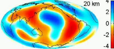
Though a neutrino beam traverses a large range of different depths, one may take this figure as an estimate of the characteristic length scales and amplitudes involved in the problem. It suggests length scales of the order of some thousands of kilometers and amplitudes of the order of $\pm 4\%$, whereas at greater depths one can indeed have somewhat larger amplitudes. In addition, the length scales and amplitudes do not seem to vary too much around their average absolute values. This also implies that the transition regions between negative and positive amplitudes are quite short compared to the overall structure. So why not simply use these measurements in neutrino physics, instead of discussing uncertainties in the Earth matter density? First, these measurements contain some averaging as well as uncertainties in the equation of state of the Earth matter density profile from the seismic wave velocity profile (see, e.g., Refs. [45, 46]). Second, different groups obtain different results [37], which are, however, not qualitatively so much different with respect to the parameters we will identify below.

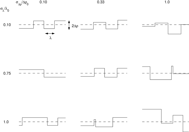
In order to model these fluctuations realistically and investigate the dependence of the relevant parameters on the neutrino oscillation transition probabilities, we use a step-function approach, varying the absolute value of the amplitude $\Delta\rho>0$ and the length scale $\lambda>0$ around some average values $\Delta\rho_{0}>0$ and $\lambda_{0}>0$ at random. For the random variation we choose a Gaussian distribution with standard deviations $\sigma_{\lambda}$ and $\sigma_{\Delta\rho}$, respectively, which is truncated at zero. Figure 3 shows some sample profiles for different values of these standard deviations and for fixed average values.

Figure 3: Sample profiles for a fixed average length scale $\lambda_{0}$ and a fixed average amplitude $\Delta\rho_{0}$, corresponding to the values in Eq. (1) and a baseline length of $L=7400\,\mathrm{km}$. The standard deviations are varied relative to the absolute values of the length scale and the amplitude.

Comparing this model with Fig. 2, we can then estimate a set of realistic parameters as

$$\lambda_{0} \sim 2000\,\mathrm{km},$$ (1a)

$$\sigma_{\lambda} \sim 1500\,\mathrm{km}=0.75\,\lambda_{0},$$ (1b)

$$\Delta\rho_{0} \sim 3\%\,\bar{\rho},$$ (1c)

$$\sigma_{\Delta\rho} \sim 1\%\,\bar{\rho}=1/3\,\Delta\rho_{0},$$ (1d)

where $\bar{\rho}=3\,\mathrm{g/cm^{3}}$ is the average matter density.

4 Numerical analysis

For physical reasons we do not expect surprises in certain regions of the parameter space. Since we cannot show the results for the whole parameter space in $\lambda_{0}$, $\Delta\rho_{0}$, $\sigma_{\lambda}$, and $\sigma_{\Delta\rho}$ simultaneously, we will now systematically investigate the dependence on some parameters by keeping the other ones fixed. One could do this by showing either the absolute errors in the appearance probabilities coming from matter density fluctuations $|\Delta P_{\alpha\beta}|$, or the relative errors $|\Delta P_{\alpha\beta}|/P_{\alpha\beta}^{\mathrm{ref}}$. For the neutrino channel $\nu_{\mu}\rightarrow\nu_{e}$, the transition probabilities are in most regions relatively large. In this case, the relative errors are quite meaningful and are usually some percent of the total probabilities. Depending on the parameters they can sometimes even be larger than $10\%$. However, for the antineutrino channel $\bar{\nu}_{\mu}\rightarrow\bar{\nu}_{e}$ the absolute probabilities in the denominators of the relative errors are rather small. Therefore, it turns out that the relative errors are not very sensible in this case. Comparing plots for the absolute and relative errors and mainly focusing on the qualitative behavior, we thus decided to show only the absolute error plots. Nevertheless, the fact that the absolute values of these errors are rather small does not mean that they are small compared to the transition probabilities. For the simulations, a large number of matter density profiles was created at random and the relative error was averaged over all computations with these profiles.

Figure 4 shows the absolute errors in the appearance probabilities for the neutrino channel, $P_{\mu e}$, and the antineutrino channel, $P_{\bar{\mu}\bar{e}}$, plotted as functions of $\sigma_{\lambda}$ for a fixed value of $\sigma_{\Delta\rho}$ and $\sigma_{\Delta\rho}$ for a fixed value of $\sigma_{\lambda}$, respectively. For the fixed parameter values we choose, if not otherwise noted, the values from Eq. (1).

Figure 4: The absolute errors in the appearance probabilities $P_{\mu e}$ and $P_{\bar{\mu}\bar{e}}$, averaged over $20000$ random matter density profiles, with the values $\lambda_{0}=2000\,\mathrm{km}$ and $\Delta\rho_{0}=3\%\cdot 3\,{\rm g/cm^{3}}$ from Eq. (1). The errors are plotted as functions of $\sigma_{\lambda}/\lambda_{0}$ for the fixed value $\sigma_{\Delta\rho}=1/3\,\Delta\rho_{0}$ (upper plot) and $\sigma_{\Delta\rho}/\Delta\rho_{0}$ for the fixed value $\sigma_{\lambda}=0.75\,\lambda_{0}$ (lower plot), respectively [cf., Eq. (1)]. The oscillation parameter values are chosen as described in the caption of Fig. 1.

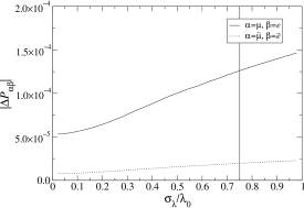
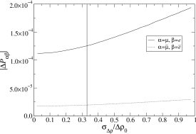
In all of our plots, the vertical lines correspond to the parameter values in Eq. (1), i.e., the same point in the multi-dimensional parameter space. Since the curves in Fig. 4 are slowly varying close to the vertical lines, we will further on take the respective values from Eq. (1) for the standard deviations. In general, the absolute errors are growing with larger fluctuations in the length scale and the amplitude. This means, in our model, that for more irregular matter density fluctuations we obtain larger errors in the transition probabilities. A possible explanation could be the zero-truncations of the Gaussian distributions, which means that for large standard deviations the average values are shifted. For antineutrinos the absolute errors are in all cases much smaller than for neutrinos, because for antineutrinos matter effects are, in general, much smaller for energies larger than a few GeV (no resonance effects).

Next, let us investigate the dependence of the absolute errors on the length scale $\lambda_{0}$ and the amplitude $\Delta\rho_{0}$. Here we choose the relative standard deviations to be $\sigma_{\lambda}=0.75\,\lambda_{0}$ and $\sigma_{\Delta\rho}=1/3\,\Delta\rho_{0}$, corresponding to Eq. (1) for the appropriate $\lambda_{0}$ and $\Delta\rho_{0}$. The result of this analysis is shown in Fig. 5, from which it can be seen that the absolute error is essentially proportional to the length scale as well as the amplitude of the fluctuations.

Figure 5: The absolute errors in the appearance probabilities $P_{\mu e}$ and $P_{\bar{\mu}\bar{e}}$, averaged over $20000$ random matter density profiles, with the standard deviation values $\sigma_{\lambda}=0.75\,\lambda_{0}$ and $\sigma_{\Delta\rho}=1/3\,\Delta\rho_{0}$, corresponding to Eq. (1). The errors are plotted as functions of the baseline fraction $\lambda_{0}/L$ for three different values of $\Delta\rho_{0}$ (upper plot) and the average matter density fraction $\Delta\rho_{0}/\bar{\rho}$ for three different values of $\lambda_{0}$ (lower plot), respectively. Note that the standard deviations scale linearly with the absolute average values. The other parameter values are chosen as described in the caption of Fig. 1.

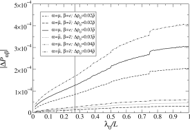
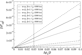
Indeed, this result is, with respect to the average length scale and amplitude, very similar to what we obtained from a single perturbation in the Earth matter density. In the latter case, we observed that the product of the length scale and amplitude determines the error in the probabilities. Thus, fixing one of these two parameters gives a linear dependence on the other one. This is, of course, only true for a single perturbation without interference effects, which means that corrections to linearity have to be taken into account in our more general model. One such interesting correction is the bumps in the upper plot. Since in our model the number of steps $n$, in which the matter density profile has been divided into, depends on the length scale, for a small number of steps $n$ the (average) transition $n\rightarrow n-1$ can be seen as a bump in the absolute errors. For large $n$ the relative contribution of this effect becomes negligible.

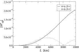
Finally, taking the parameter values as given in Eq. (1), the absolute errors in the appearance probabilities $P_{\mu e}$ and $P_{\bar{\mu}\bar{e}}$ are plotted as functions of energy and baseline in Fig. 6.

Figure 6: The absolute errors in the appearance probabilities $P_{\mu e}$ and $P_{\bar{\mu}\bar{e}}$, averaged over $20000$ random matter density profiles, with the parameter values from Eq. (1). The errors are plotted as functions of the energy $E$ for a baseline of $L=7400\,\mathrm{km}$ (upper plot) and the baseline $L$ for an energy of $E=30\,\mathrm{GeV}$ (lower plot). The other parameter values are chosen as described in the caption of Fig. 1.

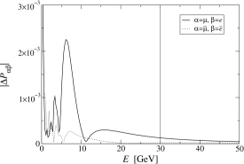
From the upper plot we can observe that the absolute errors are rather small for large energies ($E\gtrsim 10\,\mathrm{GeV}$) and so are the relative errors at least for neutrinos. Since for a neutrino factory the energy spectrum for muon neutrinos is peaked at the maximum energy [31, 32], the low-energy contributions contain less statistical information. This point supports our focus on high energies in most of the plots.

As far as the baseline dependence in the lower plot of Fig. 6 is concerned, the absolute errors are vanishing for small baselines, because matter effects become, in general, negligible. Although the neutrino and antineutrino curves look quite different in this plot, the basic principle of the shapes is the same. They are both periodic functions of the baseline, as can easily be seen for the antineutrinos, and the difference is only due to different period and amplitude.

5 Summary and conclusions

In this paper, we first investigated the effects of a single perturbation in the average matter density of the Earth (especially the Earth’s mantle). We then introduced a model for the description of random matter density fluctuations in the Earth’s mantle, which is based on the observations obtained from geophysical measurements. Finally, we used this model to analyze the dependence of the absolute errors in the appearance probabilities $P_{\mu e}$ and $P_{\bar{\mu}\bar{e}}$, especially important for long baseline neutrino factory CP measurements, on our model parameters.

We observed that, in particular for neutrinos, the absolute error in the appearance probability for random matter density fluctuations can be quite substantial, corresponding to relative errors of some few percent. The error is essentially directly proportional to the product of the amplitude and length scale of a single perturbation or the random fluctuations. Furthermore, for short baselines $L\lesssim 1000\,\mathrm{km}$, the errors are vanishing for both neutrinos and antineutrinos which means that matter density fluctuations can in this case be regarded as second order effects compared to the small matter effects.

Finally, we comment on the three possible scenarios suggested in the summary of Ref. [47]:

1. The uncertainty of present density models poses no significant problems.

2. Moderate reduction of the uncertainty, through more detailed analysis of data, is required.

3. Significant reduction of this uncertainty, by conducting a large scale campaign of geophysical observations, is required.

From our analysis, scenario (2) best fits our conclusions. In our calculations with randomly generated matter density profiles, we assumed that the fluctuations are completely unknown and we obtained relative errors of the order of magnitude of some few percent. Comparing the results of the measurements of the PREM profile corrections of different groups [37] indicates that there is not yet sufficient agreement on the data. Moderate reduction of the uncertainty by a more detailed analysis of data should help to settle this problem for neutrino physics.

Appendix A A perturbation theoretical approach to a single perturbation in the Earth matter density

In perturbation theory, we can show that for a single perturbation with constant amplitude $\Delta A\equiv\pm 2\,\sqrt{2}\,G_{F}\,E\,\Delta n_{e}\propto\Delta\rho$ in the average Earth matter density $A\propto\bar{\rho}$, the first order perturbation term is proportional to the “area” $\Delta S\equiv\lambda\,\Delta A\propto\lambda\,\Delta\rho$ of the perturbation, i.e., the length scale $\lambda$ times the amplitude $\Delta A$.

The Hamiltonian for the propagation of the neutrinos is

$$\mathcal{H}(r)=\mathcal{H}_{0}+A\,\mathcal{K}+\Delta A\,\mathcal{K}\equiv\mathcal{H}+\Delta A\,\mathcal{K},$$ (2)

where $\mathcal{K}\equiv|\nu_{e}\rangle\langle\nu_{e}|$ is the projector onto the flavor state $|\nu_{e}\rangle$. Let $\mathcal{V}(r)=e^{-i\mathcal{H}r}=\sum_{a=1}^{3}e^{-i\xi_{a}r}\,\mathcal{P}_{a}$ be the unperturbed evolution operator, where $\mathcal{P}_{a}\equiv|\nu_{a}\rangle\langle\nu_{a}|$ is the projector onto the mass eigenstate $|\nu_{a}\rangle$ with the eigenvalue $\xi_{a}$ in matter. Then the evolution operator of the full evolution equation can, to first order in perturbation theory, be written as

$$\mathcal{U}(r)\simeq\mathcal{V}(r)-i\mathcal{V}(r)\,\Delta A\sum_{a=1}^{3}\sum_{b=1}^{3}f_{ab}\,\mathcal{P}_{a}\,\mathcal{K}\,\mathcal{P}_{b},$$ (3)

where

$$f_{ab}\equiv\lambda\,e^{i(\xi_{a}-\xi_{b})r_{0}}\,\frac{\sin\left(\xi_{a}-\xi_{b}\right)\frac{\lambda}{2}}{\left(\xi_{a}-\xi_{b}\right)\frac{\lambda}{2}}$$ (4)

and $r_{0}$ is the position of the center of the fluctuation. For a fluctuation length $\lambda$, which is much shorter than the oscillation length, i.e., $(\xi_{a}-\xi_{b})(\lambda/2)\ll 1$, the last factor in Eq. (4) is approximately equal to unity. We then obtain

$$f_{ab}\simeq\lambda\,e^{i(\xi_{a}-\xi_{b})r_{0}}.$$ (5)

With this result it is easy to see that the transition probability $P_{\alpha\beta}(r)$ at the position $r$ can be written as

$$P_{\alpha\beta}(r)\simeq P^{0}_{\alpha\beta}(r)+2\,\Delta S\,\Im[X^{*}(r)Y(r)],$$ (6)

where $P^{0}_{\alpha\beta}(r)$ is the unperturbed transition probability in constant matter density, $X(r)\equiv\langle\nu_{\beta}|\mathcal{V}(r)|\nu_{\alpha}\rangle$, and $Y(r)\equiv\langle\nu_{\beta}|\left(\mathcal{V}(r_{0}-r)\right)^{\dagger}|\nu_{e}\rangle\langle\nu_{e}|\mathcal{V}(r_{0})|\nu_{\alpha}\rangle$. This shows that the perturbary contribution to the transition probability is proportional to $\Delta S$, and therefore, largely independent of the form of the perturbation. Note that perturbation theory only holds for $\Delta S$ small compared to $\langle\mathcal{H}\rangle\,r\simeq A\,r$, i.e., $\Delta A/A\ll r/\lambda$.

References

- [1] S.P. Mikheyev and A.Yu. Smirnov, Yad. Fiz. 42 (1985) 1441, [Sov. J. Nucl. Phys. 42 (1985) 913].
- [2] S.P. Mikheyev and A.Yu. Smirnov, Nuovo Cimento C 9 (1986) 17.
- [3] L. Wolfenstein, Phys. Rev. D17 (1978) 2369.
- [4] V.K. Ermilova, V.A. Tsarev and V.A. Chechin, Pis’ma Zh. Eksp. Teor. Fiz. 43 (1986) 353, [JETP Lett. 43 (1986) 453].
- [5] A.J. Baltz and J. Weneser, Phys. Rev. D35 (1987) 528.
- [6] A. Nicolaidis, Phys. Lett. B200 (1988) 553.
- [7] P.I. Krastev and S.T. Petcov, Phys. Lett. B205 (1988) 84.
- [8] T.K. Kuo and J. Pantaleone, Rev. Mod. Phys. 61 (1989) 937.
- [9] P.I. Krastev and A.Yu. Smirnov, Phys. Lett. B226 (1989) 341.
- [10] Y. Minorikawa and K. Mitsui, Europhys. Lett. 11 (1990) 607.
- [11] S.T. Petcov, Phys. Lett. B434 (1998) 321, hep-ph/9805262, ibid. B444 (1998) 584(E).
- [12] E.Kh. Akhmedov, Nucl. Phys. B538 (1999) 25, hep-ph/9805272.
- [13] E.Kh. Akhmedov et al., Nucl. Phys. B542 (1999) 3, hep-ph/9808270.
- [14] M.V. Chizhov and S.T. Petcov, Phys. Rev. Lett. 83 (1999) 1096, hep-ph/9903399.
- [15] M.V. Chizhov and S.T. Petcov, Phys. Rev. D63 (2001) 073003, hep-ph/9903424.
- [16] E.Kh. Akhmedov, Pramana 54 (2000) 47, hep-ph/9907435.
- [17] M. Freund and T. Ohlsson, Mod. Phys. Lett. A15 (2000) 867, hep-ph/9909501.
- [18] T. Ohlsson and H. Snellman, J. Math. Phys. 41 (2000) 2768, hep-ph/9910546, ibid. 42 (2001) 2345(E).
- [19] T. Ohlsson and H. Snellman, Phys. Lett. B474 (2000) 153, hep-ph/9912295, ibid. B480 (2000) 419(E).
- [20] M. Freund et al., Nucl. Phys. B578 (2000) 27, hep-ph/9912457.
- [21] I. Mocioiu and R. Shrock, Phys. Rev. D62 (2000) 053017, hep-ph/0002149.
- [22] M. Freund, P. Huber and M. Lindner, Nucl. Phys. B585 (2000) 105, hep-ph/0004085.
- [23] K. Dick et al., Nucl. Phys. B598 (2001) 543, hep-ph/0008016.
- [24] E.Kh. Akhmedov, Phys. Atom. Nucl. 64 (2001) 787, hep-ph/0008134.
- [25] T. Ota and J. Sato, Phys. Rev. D63 (2001) 093004, hep-ph/0011234.
- [26] K. Takahashi, M. Watanabe and K. Sato, Phys. Lett. B510 (2001) 189, hep-ph/0012354.
- [27] T. Ohlsson and H. Snellman, Eur. Phys. J. C20 (2001) 507, hep-ph/0103252.
- [28] T. Ohlsson, Phys. Lett. B522 (2001) 280, hep-ph/0109003.
- [29] J. Bernabeu et al., hep-ph/0110071.
- [30] K. Takahashi and K. Sato, hep-ph/0110105.
- [31] S. Geer, Phys. Rev. D57 (1998) 6989, hep-ph/9712290, ibid. D59 (1999) 039903(E).
- [32] V. Barger, S. Geer and K. Whisnant, Phys. Rev. D61 (2000) 053004, hep-ph/9906487.
- [33] A.M. Dziewonski and D.L. Anderson, Phys. Earth Planet. Inter. 25 (1981) 297.
- [34] K. Aki and P.G. Richards, Quantitative Seismology: Theory and Methods (W. H. Freeman, San Francisco, 1980), Vol. 1, 2.
- [35] T. Lay and T.C. Wallace, Modern Global Seismology (Academic Press, New York, 1995).
- [36] P.M. Shearer, Introduction to Seismology (Cambridge, Cambridge, 1999).
-
[37]
S.V. Panasyuk,
REM (Reference Earth Model) web page,
http://cfauvcs5.harvard.edu/lana/rem/
index.htm. - [38] K. Bullen, The Earth’s Density (Chapman & Hall, London, 1975).
- [39] B.L.N. Kennett, Geophys. J. Int. 132 (1998) 374.
- [40] E.Kh. Akhmedov, Phys. Lett. B503 (2001) 133, hep-ph/0011136.
- [41] L.Y. Shan, B.L. Young and X. Zhang, hep-ph/0110414.
- [42] T. Ohlsson and W. Winter, Phys. Lett. B512 (2001) 357, hep-ph/0105293.
- [43] M. Freund, P. Huber and M. Lindner, Nucl. Phys. B615 (2001) 331, hep-ph/0105071.
- [44] G. Ekström and A.M. Dziewonski, Nature 394 (1998) 168.
- [45] R. Jeanlow and S. Morris, Ann. Rev. Earth Plan. Sci. 14 (1986) 377.
- [46] R. Jeanlow, Ann. Rev. Earth Plan. Sci. 18 (1990) 357.
- [47] R.J. Geller and T. Hara, hep-ph/0111342.