Lepton Flavor Violation in the SUSY-GUT Models
with Lopsided Mass Matrix

Abstract

The tiny neutrino masses measured in the neutrino oscillation experiments can be naturally explained by the supersymmetric see-saw mechanism. If the supersymmetry breaking is mediated by gravity, the see-saw models may predict observable lepton flavor violating effects. In this work, we investigate the lepton flavor violating process $\mu\to e\gamma$ in the kind of neutrino mass models based on the idea of the “lopsided” form of the charged lepton mass matrix. The constraints set by the muon anomalous magnetic moment are taken into account. We find the present models generally predict a much larger branching ratio of $\mu\to e\gamma$ than the experimental limit. Conversely, this process may give strong constraint on the lepton flavor structure. Following this constraint we then find a new kind of the charged lepton mass matrix. The feature of the structure is that both the elements between the $2-3$ and $1-3$ generations are “lopsided”. This structure produces a very small $1-3$ mixing and a large $1-2$ mixing in the charged lepton sector, which naturally leads to small $Br(\mu\to e\gamma)$ and the LMA solution for the solar neutrino problem.

I introduction

There are two remarkable features of the neutrino parameters measured in the atmospheric and solar neutrino fluxes experiments, i.e., the extreme smallness of the neutrino masses and the large neutrino mixing angles. The maximal atmospheric neutrino mixing and the large mixing angle MSW solution of the solar neutrinos (LMA) are most favored by the present experimental datalma . The two features show that neutrinos have quite different properties compared with quarks and charged leptons. It is hoped that understanding the neutrino flavor structure may give important feedback on, or even be the key to solve, the flavor problem, which includes how to understand the observed quark and charged lepton spectrum and mixing.

Great enthusiasm has been stimulated on studying the neutrino physics and hundreds of models have been built and published in the recent yearsbarr . All the authors tried to reflect the two notable features in their neutrino mass models. The smallness of the neutrino masses is quite well understood now. See-saw mechanism seems the most natural and economic way to present tiny neutrino masses. It is interesting to notice that the study of neutrino physics may provide us some information at very high energy scale in the see-saw models.

As for the large mixing angles, it is fare to say that no satisfying and generally accepted explanation is found until now; still, much progress has been achieved in this aspect. As we know that the neutrino mixing is actually the mismatch between the bases of the charged leptons and the active left-handed (LH) neutrinos, the neutrino models depending on the see-saw mechanism are generally divided into two classes according to the origin of the large mixing angles coming from, i.e., those from the right-handed (RH) neutrino Majorana mass matrix $M_{R}$, and transferring to the active LH neutrinos through the see-saw mechanism,

$$M_{\nu}=-M_{N}M_{R}^{-1}M_{N}^{T}\ \ ,$$ (1)

where $M_{N}$ is the neutrino Dirac mass matrix, and those from the charged lepton mass matrix $M_{L}$.

See-saw mechanism is usually achieved in a supersymmetric grand unified model, which has the advantage of gauge couplings unification and avoidance of the standard model hierarchy problem as well. Since leptons and quarks are placed in the same multiplets in grand unified models and their mass matrices are related together, the question “How to keep small quark mixing while having large neutrino mixing” is raised. The first class of models can naturally keep small quark mixing because large neutrino mixing is from the RH Majorana neutrino mass matrix $M_{R}$, which is unrelated to the quark sector. Several models are built based on this idea by different choice of the form of $M_{R}$ and give satisfied predictionsfirst . As for the second class of neutrino models, to avoid large quark mixing, $M_{L}$ is usually chosen very asymmetric, or “lopsided”. Then the large LH lepton mixing is related to the large RH quark mixing, which is unobservable. A large number of models have been built based on this elegant ideaalbright ; order ; lopsid .

Neutrino oscillation means the neutrino flavor number is broken, which is conserved in the standard model (SM) as an “accidental” global symmetry. Lepton flavor number is another conserved quantum number as a global symmetry in the SM. However, it is believed that the SM is only a low energy effective theory and it must be extended to a fundamental theory at the high energy scale. These global symmetries are then broken in most extensions of the SM. Especially the non-zero neutrino masses will also break the lepton flavor symmetry and lead to lepton flavor violating (LFV) processes, such as $\mu\to e\gamma$, $\mu-e$ conversion, $\mu\to eee$, $\tau\to\mu\gamma$, $\tau\to e\gamma$, $Z\to\mu\tau$ and so on. On one hand, the LFV processes are closely related to the neutrino oscillations. On the other hand, they provide different information of the lepton flavor structure. Combining study of the two kinds of processes may give us more comprehensive understanding of the lepton flavor structure, even leading us to distinguish the origin of the large neutrino mixing angles. At least, the LFV processes may give strong constraints on the neutrino mass models since they are measured quite accurately and the sensitivity will be increased by three or more orders of magnitude in the near futuremueg ; exp ; nexp .

Recently there appear several works on the topic of lepton flavor violation based on supersymmetric see-saw modelscasas ; baek ; carv ; sato . These works either give predictions of the LFV processes based on a specific neutrino mass model or give a general analysis based on the neutrino oscillation experimental data and the assumptions of the form of the RH neutrino mass matrix. For example, Ref. casas discusses the branching ratio of $\mu\to e\gamma$ when the RH neutrinos are degenerate or completely hierarchical so that only the heaviest eigenvalue is relevant to the form of $M_{\nu}$. Under these assumptions the LFV effects are directly related to the neutrino oscillation parameters. Actually many viable models do not belong to these kinds. A general discussion of LFV for all neutrino models may be very difficult. In our work, we focus on the LFV effects of the kind of neutrino mass models exist in the literature based on the idea of “lopsided” form of the charged lepton mass matrices. In this kind of models where the large $\nu_{\mu}-\nu_{\tau}$ mixing in neutrino oscillation is actually due to the mixing in the mass matrix of the charged leptons, instead of the neutrinos, it is thus natural to expect large LFV effects. In one of our previous works we calculated the branching ratios of $\tau\rightarrow\mu\gamma$ and $Z\rightarrow\tau\mu$ generally in the “lopsided” models, independent of the model details and concluded that the process $\tau\rightarrow\mu\gamma$ might be detected in the next generation experimentsbi . We will show in this work that the branching ratio of $\mu\rightarrow e\gamma$ is already larger than the present experimental limit in typical models of this kind proposed in the literature. We then take $Br(\mu\rightarrow e\gamma)$ as a constraint which must be satisfied by the models and find an interesting structure of the charged lepton mass matrix. The notable feature of this model is that in addition to the large $2-3$ element of the matrix the $1-3$ element is of order 1 too. This structure can suppress the branching ratio of $\mu\rightarrow e\gamma$ and lead to the LMA solution of the solar neutrino problem at the same time.

Since there is strong correlation between the muon radiative decay and the muon anomalous magnetic dipole moment ($g_{\mu}-2$), we furthermore consider the constraints on the SUSY parameter space set by the recent BNL E821 experimentbnl . After the correction to the sign of the light-by-light term in the theoretical calculationsmusign , there is only a 1.6$\sigma$ discrepancy between the measured value of the muon anomalous magnetic dipole moment and the value predicted in the SMng2 .

The paper is organized as follows. The Sec. II explains how the LFV effects are produced in the supersymmetric see-saw models and presents some analytic results of our calculation. In Sec III we explain the basic idea of “lopsided” models and show the numerical results of $Br(\mu\to e\gamma)$ predicted by the models. We then present our new model in Sec IV and its predictions of $Br(\mu\to e\gamma)$. Finally we give a conclusion of our work and discuss the implications of the future experimental results of LFV processes in Sec V.

II some analytic results

II.1 Origin of LFV and related formulas

In the pure SM the lepton flavor is strictly conserved. If the SM is extended with massive and non-degenerate neutrinos, as suggested by the atmospheric and solar neutrino fluxes experiments, the LFV processes may be induced, in analogy to the Kobayashi-Maskawa (KM) mechanism. However, such processes are highly suppressed due to the smallness of the neutrino masses. The branching ratio is proportional to ${\delta M^{2}_{\nu}}/{M^{2}_{W}}$ which is hopeless to be observed early .

When supersymmetry enters the theory the scene changes completely. The LFV may also be induced through the generation mixing of the soft breaking terms in the lepton sector, i.e., the off-diagonal terms of the slepton mass matrices $(m^{2}_{\tilde{L}})_{ij}$, $(m^{2}_{\tilde{R}})_{ij}$ and the trilinear coupling $A^{L}_{ij}$. However, the present experimental bounds on the LFV processes give very strong constraints on these off-diagonal terms, with the strongest constraint coming from $BR(\mu\to e\gamma)$ ($<1.2\times 10^{-11}$)mueg .

A generally adopted way to avoid these dangerous off-diagonal terms is to impose the universality constraints on the soft terms at the SUSY breaking scale, such as in the gravity-mediatedsgra or gauge-mediatedgmsb SUSY breaking scenarios. The universality assumption is certainly the most conservative supposition we can make when we analyze the LFV effects. Under the universality assumption off-diagonal terms can be induced through quantum effects by the lepton flavor changing operators existing at high energy scale, which are necessary to produce the neutrino mixing.

We calculate these off-diagonal soft terms in the see-saw models, starting from the universal initial values at the GUT scale, by numerically solving the renormalization group equations (RGEs).Then we calculate the branching ratio of $\mu\to e\gamma$ induced by these terms.

In a supersymmetric see-saw model, the RH neutrinos are active at the energy scale above $M_{R}$(We will use the same symbol as the RH Majorana mass matrix $M_{R}$ to represent the energy scale). The superpotential of the lepton sector is then given by

$$W=Y_{N}^{ij}\hat{H}_{2}\hat{L}_{i}\hat{N}_{j}+Y_{L}^{ij}\hat{H}_{1}\hat{L}_{i}\hat{E}_{j}+\frac{1}{2}M_{R}^{ij}\hat{N}_{i}\hat{N}_{j}+\mu\hat{H}_{1}\hat{H}_{2}\ \ ,$$ (2)

where $Y_{N}$ and $Y_{L}$ are the neutrino and charged lepton Yukawa coupling matrices respectively, $i$, $j$ are the generation indices. In general, $Y_{N}$ and $Y_{L}$ can not be diagonalized simultaneously and lead to LFV interactions. The three matrices $Y_{N}$, $Y_{L}$ and $M_{R}$ can be diagonalized by

$$Y^{\delta}_{L} = U_{L}^{\dagger}Y_{L}U_{R}\ \ ,$$ (3)

$$Y^{\delta}_{N} = V_{L}^{\dagger}Y_{N}V_{R}\ \ ,$$ (4)

$$M_{R}^{\delta} = X^{T}M_{R}X\ \ ,$$ (5)

respectively, where $U_{L,R}$ , $V_{L,R}$ and $X$ are unitary matrices. The RH neutrinos can be easily integrated out one by one on the bases where $M_{R}$ is diagonal and then the relation (1) is recovered. Define

$$V_{D}=U_{L}^{\dagger}V_{L}\ ,$$ (6)

which is analog to the KM matrix $V_{KM}$ in the quark sector. Then $V_{D}$ determines the lepton flavor mixing. We can see that $V_{D}$ is determined by the LH mixing of the Yukawa coupling matrices $Y_{L}$ and $Y_{N}$ and only exists above the scale $M_{R}$. The MNS mixing matrix, which describes the low energy neutrino mixing, is defined by

$$V_{MNS}=U_{L}^{\dagger}U_{\nu},$$ (7)

where $U_{\nu}$ is the unitary matrix diagonalizing the neutrino mass matrix $M_{\nu}$ in Eq. (1). If $V_{MNS}$ and $V_{D}$ are both determined by the neutrino oscillation and LFV experiments respectively, it is possible to infer whether the large neutrino mixing is coming from the charged lepton sector or not. We can furthermore learn some information about the structure of the RH neutrino mass matrix.

The corresponding soft breaking terms for the lepton sector are rosiek

$${\cal{L}}_{soft} = -m_{H_{1}}^{2}H_{1}^{\dagger}H_{1}-m_{H_{2}}^{2}H_{2}^{\dagger}H_{2}-(m_{\tilde{L}}^{2})^{ij}\tilde{L}_{i}^{\dagger}\tilde{L}_{j}-(m_{\tilde{E}}^{2})^{ij}\tilde{E}_{i}^{*}\tilde{E}_{j}-(m_{\tilde{N}}^{2})^{ij}\tilde{N}_{i}^{*}\tilde{N}_{j}$$ (8)

$$+\left(B\mu H_{1}H_{2}+\frac{1}{2}BM_{R}^{ij}\tilde{N}_{i}^{*}\tilde{N}_{j}^{*}+(A^{L}Y_{L})^{ij}H_{1}\tilde{L}_{i}\tilde{E}_{j}\right.$$

$$\left.+(A^{N}Y_{N})^{ij}H_{2}\tilde{L}_{i}\tilde{N}_{j}+h.c.\right)\ \ .$$

We assume the universal condition at the GUT scale

$$m_{H_{1}}^{2} = m_{H_{1}}^{2}=m_{0}^{2}\ \ ,$$ (9)

$$m_{\tilde{L}}^{2} = m_{\tilde{R}}^{2}=m_{\tilde{N}}^{2}=m_{0}^{2}\ \ ,$$ (10)

$$A^{L} = A^{N}=A_{0}\ \ .$$ (11)

The above LFV effects in the superpotential, determined by $V_{D}$, then transfer to the soft terms through quantum effects and induce non-diagonal terms from the initial universal form. This is clearly shown by the following RGE for $m_{\tilde{L}}^{2}$, which gives the dominant contribution to the low energy LFV processes,

$$\mu\frac{dm_{\tilde{L}}^{2}}{d\mu} = \frac{2}{16\pi^{2}}\left[-\Sigma c_{i}g_{i}^{2}M_{i}^{2}+\frac{1}{2}[Y_{N}Y_{N}^{\dagger}m_{\tilde{L}}^{2}+m_{\tilde{L}}^{2}Y_{N}Y_{N}^{\dagger}]+\frac{1}{2}[Y_{L}Y_{L}^{\dagger}m_{\tilde{L}}^{2}+m_{\tilde{L}}^{2}Y_{L}Y_{L}^{\dagger}]\right.$$ (12)

$$\left.+Y_{L}m_{\tilde{E}}^{2}Y_{L}^{\dagger}+m_{H_{D}}^{2}Y_{L}Y_{L}^{\dagger}+E_{A}E_{A}^{\dagger}+Y_{N}m_{\tilde{N}}^{2}Y_{N}^{\dagger}+m_{H_{U}}^{2}Y_{N}Y_{N}^{\dagger}+N_{A}N_{A}^{\dagger}\right]$$

with $E_{A}=A^{L}\cdot Y_{L}$, $N_{A}=A^{N}\cdot Y_{N}$ and $g_{i}$, $M_{i}$ being the gauge coupling constants and gaugino masses respectively.

In the basis where $Y_{L}$ and $M_{R}$ are diagonal, an approximate formula for the off-diagonal terms of $m_{\tilde{L}}^{2}$ applicable for $\delta m^{2}\ll m_{0}^{2}$ is given by

$$\left(\delta m_{\tilde{L}}^{2}\right)_{ij} \approx \frac{1}{8\pi^{2}}(Y_{N}Y_{N}^{\dagger})_{ij}(3+a^{2})m_{0}^{2}\log\frac{M_{GUT}}{({M_{R}})_{3}}+\cdots$$ (13)

$$\approx \frac{1}{8\pi^{2}}(V_{D})_{i3}(V_{D}^{*})_{j3}\cdot Y_{N_{3}}^{2}(3+a^{2})m_{0}^{2}\log\frac{M_{GUT}}{({M_{R}})_{3}}+\cdots\ \ ,$$

where in the diagonalized Yukawa matrix $Y_{N}^{\delta}$ only the (3,3) element $Y_{N_{3}}$ is kept under the assumption of a hierarchical form of $Y_{N}$. We will use the GUT-motivated assumption $Y_{N_{3}}\approx Y_{t}$ as an order estimate. The ‘$a$’ is the universal trilinear coupling given by $A_{0}=am_{0}$. $({M_{R}})_{3}$ is the mass of the heaviest RH neutrino. The ellipsis dots ‘$\cdots$’ in Eq. (13) represent the corrections due to the RGE running below the scale $({M_{R}})_{3}$, where the heaviest RH neutrino is decoupled. If there is large mixing between the first two generations and the third generation in $V_{R}^{\dagger}X$, for example, the large $2-3$ mixing, we will have another two terms besides the term in Eq. (13), i.e.,

$$\frac{1}{8\pi^{2}}(V_{D})_{i3}(V_{D}^{*})_{j3}\cdot Y_{N_{3}}^{2}(3+a^{2})m_{0}^{2}\left((1-|(V_{R}^{\dagger}X)_{33}|^{2})\log\frac{({M_{R}})_{3}}{({M_{R}})_{2}}+|(V_{R}^{\dagger}X)_{31}|^{2}\log\frac{({M_{R}})_{2}}{({M_{R}})_{1}}\right).$$ (14)

The above term is negligible in the case of $V_{R}^{\dagger}X\approx 1$.

II.2 Some analytic formulas

In this subsection we give the analytic expressions for the branching ratio of the LFV process $\mu\to e\gamma$ and the muon anomalous magnetic dipole moment within the supersymmetric framework.

Figure 1: Feynman diagrams for the process $\mu\to e\gamma$ by exchanging charginos and neutralinos respectively.

The LFV decay of muon occurs through photon-penguin diagrams including sleptons, neutralinos and charginos, shown in FIG. 1. The amplitude of the charged lepton radiative decay can be written in a general form

$$M=em_{i}\bar{u}_{j}(p_{j})i\sigma_{\mu\nu}q^{\nu}(A^{ij}_{L}P_{L}+A^{ij}_{R}P_{R})u_{i}(p_{i})\epsilon^{\mu}(q)\ \ ,$$ (15)

where $P_{L,R}=\frac{1}{2}(1\mp\gamma_{5})$ are the chirality projection operators. The $i$, $j$ represent initial and final lepton flavors respectively. The most convenient way to calculate $A_{L}$ and $A_{R}$ is to pick up the one loop momentum integral contributions which are proportional to $\bar{u}_{j}(p_{j})P_{L,R}u_{i}(p_{i})2p_{i}\cdot\epsilon$ respectively. The neutralino exchanging contribution is

$$A_{L}^{(n)} = -\frac{1}{32\pi^{2}}(\frac{e}{\sqrt{2}\cos\theta_{W}})^{2}\frac{1}{m_{\tilde{l}_{\alpha}}^{2}}\left[{B^{j\alpha a}}^{*}B^{i\alpha a}F_{1}(k_{\alpha a})+\frac{m_{\chi_{a}^{0}}}{m_{i}}{B^{j\alpha a}}^{*}A^{i\alpha a}F_{2}(k_{\alpha a})\right]\ ,$$ (16)

$$A_{R}^{(n)} = A_{L}^{(n)}\ (B\leftrightarrow A)\ ,$$ (17)

where

$$F_{1}(k) = \frac{1-6k+3k^{2}+2k^{3}-6k^{2}\log k}{6(1-k)^{4}}\ \ ,$$ (18)

$$F_{2}(k) = \frac{1-k^{2}+2k\log k}{(1-k)^{3}}\ \ ,$$ (19)

with $k_{\alpha a}={m_{\chi_{a}^{0}}^{2}}/{m_{\tilde{l}_{\alpha}}^{2}}$. $A$ and $B$ are the lepton–slepton–neutralino coupling vertices given by

$$A^{i\alpha a} = \left(Z_{\tilde{L}}^{i\alpha}(Z_{N}^{1a}+Z_{N}^{2a}\cot\theta_{W})-\cot\theta_{W}\frac{m_{l_{i}}}{M_{W}\cos\beta}Z_{\tilde{L}}^{(i+3)\alpha}{Z_{N}^{3a}}\right)\ \ ,$$ (20)

$$B^{i\alpha a} = -\left(2Z_{\tilde{L}}^{(i+3)\alpha}{Z_{N}^{1a}}^{*}+\cot\theta_{W}\frac{m_{l_{i}}}{M_{W}\cos\beta}Z_{\tilde{L}}^{i\alpha}{Z_{N}^{3a}}^{*}\right)\ \ ,$$ (21)

with $Z_{\tilde{L}}$ being the $6\times 6$ slepton mixing matrix and $Z_{N}$ being the neutralino mixing matrix given in Ref. rosiek ; bi . The corresponding contribution coming from exchanging charginos is

$$A_{L}^{(c)} = \frac{g_{2}^{2}}{32\pi^{2}}{Z_{\tilde{\nu}}^{i\alpha}}^{*}Z_{\tilde{\nu}}^{j\alpha}\frac{1}{m_{\tilde{\nu}_{\alpha}}^{2}}\left[Z^{-}_{2a}{Z^{-}_{2a}}^{*}\frac{m_{i}m_{j}}{2M_{W}^{2}\cos^{2}\beta}F_{3}(k_{\alpha a})\right.$$ (22)

$$\left.+\frac{m_{\chi^{-}_{a}}}{\sqrt{2}M_{W}\cos\beta}Z^{+}_{1a}Z^{-}_{2a}\frac{m_{j}}{m_{i}}F_{4}(k_{\alpha a})\right]\ \ ,$$

$$A_{R}^{(c)} = \frac{g_{2}^{2}}{32\pi^{2}}{Z_{\tilde{\nu}}^{i\alpha}}^{*}Z_{\tilde{\nu}}^{j\alpha}\frac{1}{m_{\tilde{\nu}_{\alpha}}^{2}}\left[Z^{+}_{1a}{Z^{+}_{1a}}^{*}F_{3}(k_{\alpha a})+\frac{m_{\chi^{-}_{a}}}{\sqrt{2}M_{W}\cos\beta}{Z^{+}_{1a}}^{*}{Z^{-}_{2a}}^{*}F_{4}(k_{\alpha a})\right]\ \ ,$$ (23)

where

$$F_{3}(k) = \frac{2+3k-6k^{2}+k^{3}+6k\log k}{6(1-k)^{4}}\ \ ,$$ (24)

$$F_{4}(k) = \frac{3-4k+k^{2}+2\log k}{(1-k)^{3}}\ \ ,$$ (25)

with $k_{\alpha a}={m_{\chi_{a}^{-}}^{2}}/{m_{\tilde{\nu}_{\alpha}}^{2}}$. $Z_{\tilde{\nu}}$, $Z^{+}$ and $Z^{-}$ are the mixing matrices of sneutrinos and charginos as given in Ref. rosiek ; bi .

The branching ratio of $\mu\to e\gamma$ is given by

$$BR(\mu\to e\gamma)=\frac{\alpha_{em}}{4\pi}m_{\mu}^{5}(|A^{12}_{L}|^{2}+|A^{12}_{R}|^{2})/\Gamma_{\mu}\ \ ,$$ (26)

with $\Gamma_{\mu}=2.996\times 10^{-19}GeV$pdg .

To identify the dominant contribution one may use the mass insertion approximationhisano ; casas . Under this approximation and when $\tan\beta$ is large we have

$$Br(\mu\to e\gamma)\ \sim\ \frac{\alpha^{3}}{G_{F}^{2}}\frac{[(m^{2}_{\tilde{L}})_{12}]^{2}}{m_{s}^{8}}\tan^{2}\beta\ \ ,$$ (27)

where $m_{s}$ represents general slepton mass and “$\sim$” means some constants are omitted on the right-hand side. From this expression we can clearly see that the supersymmetric contribution to $Br(\mu\to e\gamma)$ is proportional to $\tan^{2}\beta$ and the first two generation slepton mass mixing.

In the computation of the LFV branching ratios we considered the constraints on the supersymmetric parameter space set by the BNL E821 experiment of the muon anomalous magnetic momentbnl . We give the related analytic formulas in the following.

The amplitude for the photon-muon-muon coupling in the limit of the photon momentum $q$ tending to zero can be written as

$$M^{\prime}=ie\bar{u}_{\mu}\left\{\gamma^{\alpha}+a_{\mu}\frac{i\sigma^{\alpha\beta}q_{\beta}}{2m_{\mu}}\right\}u_{\mu}\epsilon_{\alpha}(q)\ \ ,$$ (28)

with $a_{\mu}$ being the muon anomalous magnetic moment. The discrepancy is give byng2

$$\delta a_{\mu}=a_{\mu}^{exp}-a_{\mu}^{SM}=26(\pm 16)\times 10^{-10}\ \ .$$ (29)

The supersymmetric contribution to $\delta a_{\mu}$ comes from the same photon-penguin diagrams producing $\mu\to e\gamma$ decay by replacing the final state by muon. The analytic expressions for $\delta a_{\mu}$ from the neutralino and chargino exchanging contributions are

$$\delta a_{\mu}^{(n)} = -\frac{1}{32\pi^{2}}\frac{e^{2}}{\cos^{2}\theta_{W}}\frac{m_{\mu}^{2}}{m_{\tilde{l}_{\alpha}}^{2}}\cdot$$ (30)

$$\left[({A^{i\alpha a}}^{*}A^{i\alpha a}+{B^{i\alpha a}}^{*}B^{i\alpha a})F_{1}(k_{\alpha a})+\frac{m_{\chi_{a}^{0}}}{m_{\mu}}Re({A^{i\alpha a}}^{*}B^{i\alpha a})F_{2}(k_{\alpha a})\right]\ \ ,$$

and

$$\delta a_{\mu}^{(c)} = \frac{g_{2}^{2}}{16\pi^{2}}\frac{m_{\mu}^{2}}{m_{\tilde{\nu}_{\alpha}}^{2}}Z_{\tilde{\nu}}^{i\alpha}{Z_{\tilde{\nu}}^{i\alpha}}^{*}\cdot$$ (31)

$$\left[({Z_{1a}^{+}}^{*}Z_{1a}^{+}+\frac{m_{\mu}^{2}}{2M_{W}^{2}\cos\beta}{Z_{2a}^{-}}^{*}Z_{2a}^{-})F_{3}(k_{\alpha a})+\frac{m_{\chi_{a}^{-}}}{\sqrt{2}M_{W}\cos\beta}Re(Z_{1a}^{+}Z_{2a}^{-})F_{4}(k_{\alpha a})\right]\ .$$

respectively.

Comparing the expressions for the amplitude of muon decay and muon anomalous magnetic moment we find a striking resemblance. Because a mass insertion is necessary to give correct fermion chirality in Eq. (15), $|A_{R}|$ dominates over the contributions. At large $\tan\beta$ a direct relation between the two quantities is then found under the mass insertion approximationcarv

$$Br(\mu\to e\gamma)\approx\frac{192\pi^{3}\alpha}{G_{F}^{2}m_{\mu}^{4}}\times(\delta a_{\mu})^{2}\times\kappa^{2}\ \ ,$$ (32)

where $\kappa\equiv A_{R}^{12}/A_{R}^{22}$. It is easy to check that Eq. (32) is consistent with Eq. (27) and $\kappa\approx({\delta m_{\tilde{L}}^{2}})_{12}/m_{s}^{2}$ if we notice that $Z_{\tilde{\nu}}^{i\alpha}({m_{\tilde{\nu}_{\alpha}}^{2}})^{-1}{Z_{\tilde{\nu}}^{j\alpha}}^{*}\approx-({\delta m_{\tilde{L}}^{2}})_{ij}/m_{s}^{4}$ with $m_{s}$ being the common slepton mass. Assuming $\delta a_{\mu}$ is due to the supersymmetric corrections, Eq. (32) may give constraints on the numerical results of the LFV branching ratio if the flavor mixing parameter $\kappa$ can be predicted in an explicit model.

III $\mu\to e\gamma$ in the “lopsided” neutrino mass models

III.1 Basic idea of “lopsided” neutrino mass models

In a SU(5) grand unified model, the LH charged leptons are in the same multiplets as the CP conjugates of the RH down quarks. This feature leads to the fact that the mass matrix for the charged leptons is related closely in form to the transpose of the mass matrix of the down quarks. The basic idea of “lopsided” models is that the charged lepton and the down quark mass matrices have the approximate forms asalbright ; order ; lopsid

$$M_{L}\ \sim\ \left(\begin{array}[]{ccc}0&0&0\\ 0&0&\sigma\\ 0&\epsilon&1\end{array}\right)m_{D},\ \ M_{D}\ \sim\ \left(\begin{array}[]{ccc}0&0&0\\ 0&0&\epsilon\\ 0&\sigma&1\end{array}\right)m_{D}$$ (33)

with $\epsilon\ll 1$ while $\sigma\sim 1$ and zeros representing small entries. In the case of the charged leptons $\sigma$ controls the mixing of the second and the third families of the LH leptons (Here we use the convention that the LH doublet multiplies the Yukawa coupling matrix from the left side while the RH singlet from the right side), which contributes to the atmospheric neutrino mixing and makes the mixing angle $\theta_{atm}$ large, while $\epsilon$ controls the mixing of the second and the third families of the RH leptons, which is not observable at low energy. For the quarks the reverse is the case: the small $\mathcal{O}(\epsilon)$ mixing is in the LH sector, accounting for the smallness of $V_{cb}$, while the large $\mathcal{O}(\sigma)$ mixing is in the RH sector, which is not observable.

The crucial element in the approach is the “lopsided” form of the mass matrices for the charged leptons and the down quarks and that $M_{L}$ being similar to the transpose of $M_{D}$. The relation $M_{L}\sim M_{D}^{T}$ can be achieved in grand unified models based on larger groups where SU(5) is a subgroup and plays the critical role to give the relation. This relation can also be achieved in models with abelian or non-abelian flavor symmetries, no matter they base on grand unification or not. Generally there is no such relationship between $M_{N}$ and the up quark mass matrix $M_{U}$ in SU(5). They are usually assumed to be not lopsided and give small mixing in the literature. However, we shall use $({M_{U}})_{33}=({M_{N}})_{33}$ in our calculation, which is valid in the simplest SO(10) model.

As for the large mixing between the first two generations in the neutrino oscillation, which is assumed to explain the solar neutrino problem, it is usually given by the LH neutrino mass matrix $M_{\nu}$ in the literaturebarr ; albright ; order ; lopsid . Thus the mixing angle $\theta_{12}$ of the LH charged leptons is usually small.

III.2 Order estimate of $\mu\to e\gamma$ in the “lopsided” models

We first give an order estimate of the branching ratio of $\mu\to e\gamma$ in the “lopsided” models. The quantitative results are given by solving the RGEs numerically and presented in the next subsection.

The starting point is Eq. (13). In the “lopsided” models there can be no large mixing in $V_{R}^{\dagger}X$ and the RGEs running below $({M_{R}})_{3}$ in Eq. (13) is ignored. Under the assumption ${Y_{N}}_{3}\approx Y_{t}$, the ratio between the off-diagonal term $(\delta m_{\tilde{L}}^{2})_{12}$ and the diagonal term, which is approximately $m_{0}$, is determined by ${(V_{D})}_{13}$, ${(V_{D})}_{23}$ and $({M_{R}})_{3}$.

$V_{D}$ is defined in Eq. (6). We estimate $V_{D}$ through an analysis similar to the analysis in Ref. barr in which the order of the MNS matrix element $U_{e3}$ is determined. Writing $U_{L}$ in the form

$$U_{L}=\left(\begin{array}[]{ccc}1&0&0\\ 0&\overline{c}_{23}&\overline{s}_{23}\\ 0&-\overline{s}_{23}&\overline{c}_{23}\end{array}\right)\left(\begin{array}[]{ccc}\overline{c}_{13}&0&\overline{s}_{13}\\ 0&1&0\\ -\overline{s}_{13}&0&\overline{c}_{13}\end{array}\right)\left(\begin{array}[]{ccc}\overline{c}_{12}&\overline{s}_{12}&0\\ -\overline{s}_{12}&\overline{c}_{12}&0\\ 0&0&1\end{array}\right),$$ (34)

where $\overline{s}_{ij}\equiv\sin\overline{\theta}_{ij}$, $\overline{c}_{ij}\equiv\cos\overline{\theta}_{ij}$ and $V_{L}$ in a similar way with the corresponding angles being denoted by $\tilde{\theta}_{ij}$, we get the expressions for $({V_{D}})_{13}$ and $({V_{D}})_{23}$,

$$({V_{D}})_{13} = -\overline{s}_{12}s_{23}\tilde{c}_{13}-\overline{s}_{13}\overline{c}_{12}c_{23}\tilde{c}_{13}+\overline{c}_{13}\overline{c}_{12}\tilde{s}_{13}\ \ ,$$ (35)

$$({V_{D}})_{23} = \overline{c}_{12}s_{23}\tilde{c}_{13}+\overline{c}_{13}\overline{s}_{12}\tilde{s}_{13}-\overline{s}_{13}\overline{s}_{12}c_{23}\tilde{c}_{13}\ \ ,$$ (36)

with $s_{23}\equiv\sin(\tilde{\theta}_{23}-\bar{\theta}_{23})$. Under the GUT-based assumption that $Y_{N}$ has a similar hierarchical structure with that of up quark, we expect that $\tilde{s}_{13}$ is of the same order as the corresponding mixing angle, $\theta_{U}^{13}$, in the up quark mixing matrix. If we further assume that no accidental cancellation exists between the up and down quark mixing matrices, we then get $\theta_{U}^{13}\lesssim V_{td}\sim 0.008$pdg , where $V_{td}$ is the 31 element of the CKM matrix. So, $\tilde{s}_{13}\lesssim 0.008$. Similarly, we have $\tilde{s}_{23}\lesssim V_{ts}\cong 0.04$. One typically finds that $\bar{s}_{12}\sim\sqrt{m_{e}/m_{\mu}}\cong 0.07$ and $\bar{s}_{13}\approx m_{\mu}/m_{\tau}\bar{s}_{12}\ll\bar{s}_{12}$barr ; frit . These two relations hold in most viable models, where $m_{\tau}$ and $m_{\mu}$ get their masses from the 2-3 block of the mass matrix. Considering that $s_{23}\sim c_{23}\sim\mathcal{O}(1)$ in the “lopsided” models then we get

$$({V_{D}})_{13} \approx -\overline{s}_{12}s_{23}\approx\bar{s}_{12}\bar{s}_{23}\approx 0.05\ \ ,$$ (37)

$$({V_{D}})_{23} \approx s_{23}\approx-\bar{s}_{23}\approx-0.71\ \ .$$ (38)

The $({V_{D}})_{13}$ and $({V_{D}})_{23}$ are actually determined by $U_{L}$ solely in the “lopsided” models. This conclusion certainly depends on the assumption of the form of $Y_{L}$ and $Y_{N}$. However, it is actually correct in most published “lopsided” modelsalbright ; order . We can actually relax this assumption, unless strong cancellation taking place in Eq. (35), we always get that $({V_{D}})_{13}$ is $\mathcal{O}(0.05)$ or larger.

$M_{R}$ is determined by using the see-saw relation Eq. (1) conversely

$$M_{R}=-M_{N}^{T}M_{\nu}^{-1}M_{N}.$$ (39)

If we assume that $M_{N}$ has similar spectrum to the up quarks and $M_{\nu}$ gives the large mixing for neutrino oscillation, i.e., $V_{L,R}\approx U_{L,R}\approx I$ and $U_{\nu}\approx V_{MNS}$, we find the scale of $M_{R}$ is actually determined by the lightest neutrino mass, with $({M_{R}})_{3}\gtrapprox 2.5\times 10^{15}GeV$. If $Y_{L}$ is lopsided and $M_{\nu}$ is approximately diagonal, i.e., $U_{L}^{\dagger}\approx V_{MNS}$ and $U_{\nu}\approx I$, the scale of $M_{R}$ is then determined by the heaviest neutrino mass, with $({M_{R}})_{3}\approx 4\times 10^{14}GeV$.

Having known the values of the elements $(V_{D})_{13}$, $(V_{D})_{23}$ and $M_{R}$, we can give the order estimation of $\mu\to e\gamma$ by a simple calculation. At the large $\tan\beta$ case, the most important contribution is coming from the second term in Eq. (23). Assuming that all the SUSY particles are of the scale $m_{s}$ we then have

$$Br(\mu\to e\gamma) \approx \frac{\alpha_{em}}{4\pi}m_{\mu}^{5}\left(\frac{g_{2}^{2}}{32\pi^{2}}\right)^{2}\left(\frac{({m^{2}_{\tilde{L}}})_{12}}{m_{s}^{4}}\right)^{2}\left|\frac{m_{\chi_{a}^{-}}Z_{1a}^{+}Z_{2a}^{-}F_{4}(k_{a})}{\sqrt{2}M_{W}}\right|^{2}\tan^{2}\beta/\Gamma_{\mu}$$ (40)

$$\approx C\cdot 10^{-7}\left(\frac{100GeV}{m_{s}}\right)^{4}\left(\frac{\tan\beta}{10}\right)^{2}\ ,$$ (41)

with $C$ being around $1\sim 10$. This estimate means that unless all the SUSY particles tend to above $1TeV$ and $\tan\beta$ is not too large the branching ratio should be above the present experimental limit. The reason for such a large branching ratio is clear: the “lopsided” structure enhances $({V_{D}})_{23}$ and $({V_{D}})_{13}$ at the same time, as shown in Eqs. (37) and (38). The branching ratio is thus approximately proportional to $\bar{s}_{23}^{4}$, which is about 2 orders larger if taking $\bar{s}_{23}\approx\sqrt{m_{\mu}/m_{\tau}}$ in the symmetric case. Then the branching ratio may be at the same order of, or be slightly below, the present experimental limit.

III.3 Numerical results

In this subsection we give the numerical results of the branching ratio of $\mu\to e\gamma$ in the “lopsided” models. When solving the RGEs we only keep the third generation Yukawa coupling eigenvalues $Y_{\tau}$ and $Y_{N_{3}}$ in $Y_{L}$ and $Y_{N}$ and ignore the contributions from the first two generations. We take $({V_{D}})_{23}=-\bar{s}_{23}=-1/\sqrt{2}$ and $({V_{D}})_{13}=\bar{s}_{12}\bar{s}_{23}=0.07/\sqrt{2}$ as the typical values in this kind of models. We also show the results when $\bar{s}_{12}$ is as small as $0.01$. Below $M_{R}$ we solve the RGEs of MSSM where $Y_{N}$ is absent. The details about solving the RGES are given in Ref. bi . We present the dependence of the results on the SUGRA parameters: $m_{0}$, $m_{1/2}$, $A_{0}$, $\tan\beta$ and the sign of $\mu$ parameter.

We first constrain the SUGRA parameter space by the following conditions: (1) electroweak spontaneous symmetry breaking is produced by radiative corrections and correct vacuum expectation value is given; (2) the LSP of the model be the lightest neutralino with its mass limit $m_{\chi^{0}_{1}}>45GeV$; (3) the lightest chargino is heavier than $94GeV$ and (4) the lightest charged slepton is heavier than $81GeV$. $\delta a_{\mu}$ gives further constraints on the parameter space. It always constrains the $\mu$ parameter to be positive. We fix $A_{0}=m_{0}$ throughout the calculation, which does not affect the result much, and take $M_{R}=4.5\times 10^{14}GeV$.

Figure 2: $\delta a_{\mu}$ as a function of $m_{0}$ for $\tan\beta=5$, $m_{1/2}=150GeV$ and for $\tan\beta=10$, $m_{1/2}=150,250GeV$ respectively. $A_{0}=m_{0}$ and $\mu>0$ are assumed. For $\mu<0$, $\delta a_{\mu}$ is negative with almost the same magnitude as the present corresponding values. The horizontal lines represent the E821 central value and it $\pm 1\sigma$ and $\pm 1.5\sigma$ bounds.

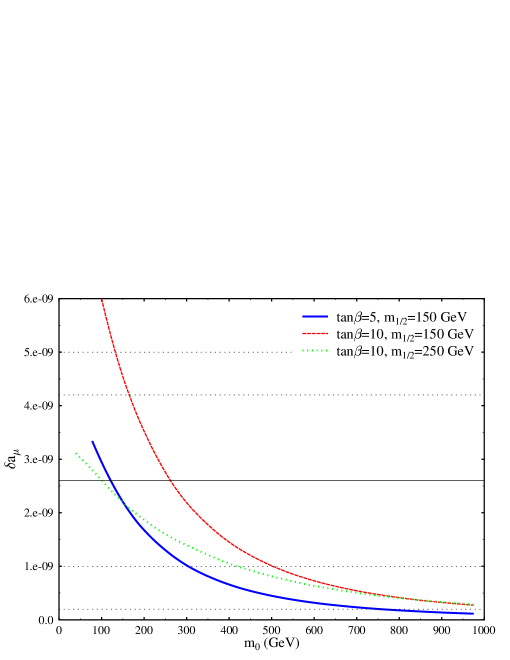
In FIG. 2 we plot $\delta a_{\mu}$ as a function of $m_{0}$ for $\tan\beta=5,10$ and $m_{1/2}=150,250GeV$ respectively. The horizontal lines are the E821 central value and its $\pm 1\sigma$ and $\pm 1.5\sigma$ bounds. $m_{1/2}=150GeV$ is almost the smallest value we can take considering the chargino mass experimental limit. We find $\mu<0$ always predicts a $\delta a_{\mu}<0$ with almost the same magnitude as the corresponding predictions for positive $\mu$.

The formulas for $\delta a_{\mu}$ we adopted, Eqs. (30) and (31), are different from those given by most authors because we use the full slepton and sneutrino mass matrices including the off-diagonal terms. The numerical results, however, do not depend on the mixing angles, just as expected. This can be regarded as a check for our program.

Figure 3: Branching ratio of $\mu\to e\gamma$ as a function of $m_{0}$ for $\tan\beta=5$, $m_{1/2}=150GeV$. $A_{0}=m_{0}$ and $\mu>0$ are assumed. $\theta_{12}$ is the mixing angle between the 1-2 generations defined in Eq. (34). The horizontal dotted line is the present experimental limit for $\mu\to e\gamma$, $1.2\times 10^{-11}$mueg .

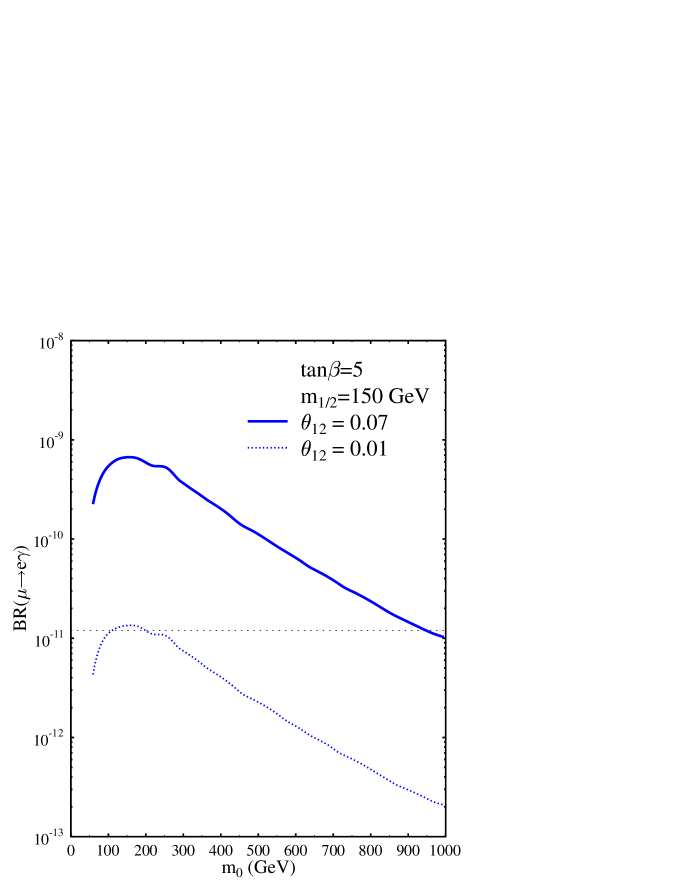
In FIG. 3 $Br(\mu\to e\gamma)$ is plotted as a function of $m_{0}$ for $\tan\beta=5$, with $m_{1/2}=150GeV$. $\theta_{12}$ represents the 1-2 mixing angle defined in Eq. (34) (We omit the bar over $\theta$ thereafter). We notice that if $\theta_{12}$ takes the typical value 0.07 in the “lopsided” models the predicted branching ratio is far larger than the present experimental limit in most parameter space. For $\tan\beta=5$ we can suppress the branching ratio below the experimental limit when we take $\theta_{12}$ as small as 0.01.

Figure 4: Branching ratio of $\mu\to e\gamma$ as a function of $m_{0}$ for $\tan\beta=10$ and $m_{1/2}=150GeV,250GeV$. Other comments are the same as that given in FIG. 3.

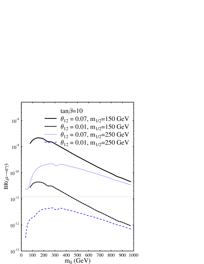
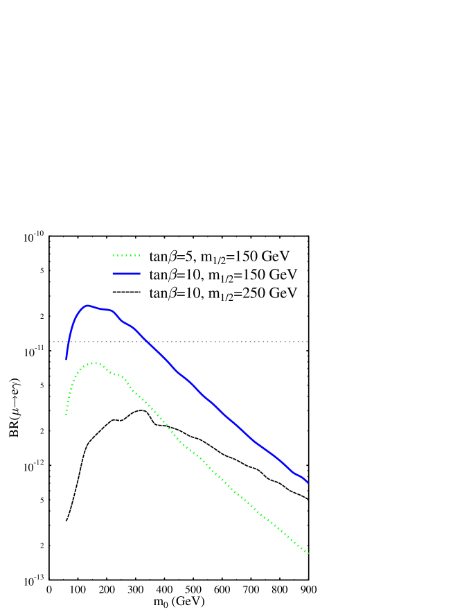
FIG. 4 plots $Br(\mu\to e\gamma)$ as a function of $m_{0}$ for $\tan\beta=10$ and $m_{1/2}=150,\ 250GeV$ respectively. For the typical value $\theta_{12}=0.07$ the predicted branching ratio is always larger than the experimental limit. In case of $m_{1/2}=150GeV$, even we take $\theta_{12}=0.01$ the predicted branching ratio is still too large for $m_{0}\lesssim 470GeV$, where $\delta a_{\mu}$ falls within the $1\sigma$ range. When $m_{1/2}$ is $250GeV$, the branching ratio can be below the experimental limit when $\theta_{12}=0.01$.

Figure 5: $\delta a_{\mu}$ as a function of $m_{0}$ for $\tan\beta=20$, $m_{1/2}=250GeV,350GeV$ respectively. Other comments are the same as that given in FIG. 2.

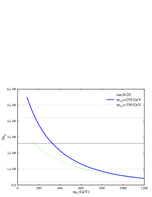
We display $\delta a_{\mu}$ as a function of $m_{0}$ for $\tan\beta=20$ in FIG. 5, with $m_{1/2}=250,350GeV$ respectively. The value of $m_{0}$ in the $\pm 1\sigma$ region can now be as large as about $700GeV$.

Figure 6: Branching ratio of $\mu\to e\gamma$ as a function of $m_{0}$ for $\tan\beta=20$, $m_{1/2}=250GeV,350GeV$. Other comments are the same as that given in FIG. 3.

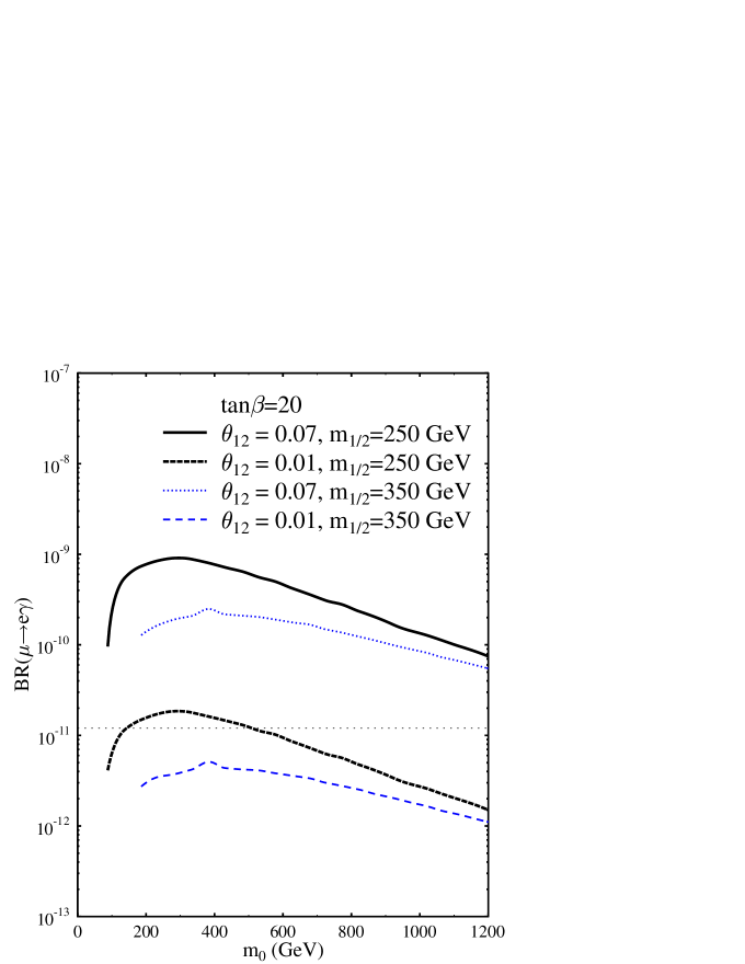
FIG. 6 is similar to FIG. 4 except that $\tan\beta=20$ and $m_{1/2}=250GeV$ and $350GeV$ now. In case of $\tan\beta=20$, we must take $m_{1/2}$ as large as $350GeV$ so that we can get a suppressed $Br(\mu\to e\gamma)$ when $\theta_{12}=0.01$ in the $\pm 1\sigma$ region of $\delta a_{\mu}$.

In summary, the branching ratio of $\mu\to e\gamma$ is sensitive to the SUSY parameters $m_{0}$, $m_{1/2}$ and $\tan\beta$. For the typical value $\theta_{12}=0.07$, in most parameter space the “lopsided” models predict a $Br(\mu\to e\gamma)$ greater than the present experimental limit. Only when $\theta_{12}$ is as small as $0.01$ can the predicted branching ratio be below the present limit. Following this consideration, we build a new kind of models which can produce a near maximal $2-3$ mixing, large $1-2$ mixing in the charged lepton sector and extremely small $({V_{D}})_{13}$.

IV An interesting form of charged lepton mass matrix

We have shown in the last section that the “lopsided” models usually predict a larger branching ratio of $\mu\to e\gamma$ than the present experimental limit. The large $2-3$ generation mixing of the charged leptons enhances both the elements $({V_{D}})_{23}$ and $({V_{D}})_{13}$. Furthermore, the scale of $M_{R}$ is lower than that in the case when the large neutrino mixing comes from $M_{\nu}$. Several authors noticed this fact and pointed out that this might imply a universal condition for the soft-SUSY breaking terms at the energy scale not much higher than the weak scalecasas ; sato , such as in the gauge mediated SUSY breaking (GMSB) models.

If we do not give up the attractive supergravity models and at the same time insist that the maximal atmospheric neutrino mixing is mainly coming from the charged lepton mixing, the sole way to suppress the process $\mu\to e\gamma$ is to suppress $({V_{D}})_{13}$. We have examined many such models with symmetric elements between the first row and the first column in the charged lepton mass matrix. We found that $\bar{s}_{12}$ is always given by $\sqrt{m_{e}/m_{\mu}}\sim 0.07$ with a coefficient of order $1$. So the model with such structure will generally give a too large branching ratio of $\mu\to e\gamma$, as shown in the last section. However, we find $({V_{D}})_{13}$ can be greatly suppressed in a new form of the charged lepton mass matrix with the elements of $1-3$ generations asymmetric. The amazing thing of this kind of models is that a large $1-3$ element in $M_{L}$ can lead to a large $1-2$ generation mixing, which leads to the LMA solution to the solar neutrino problem, and a very small $({V_{D}})_{13}$ at the same time. As shown in Ref. barr , the LMA solution is usually difficult to be constructed and most neutrino mass models predict a SMA or VO solution for the solar neutrinos. The reason for this is that most models try to produce both the large $1-2$ mixing, with $\tan^{2}\theta_{sol}$ in the range from about 0.2 to 0.8, and the small ratio of mass-squared split $\Delta m^{2}_{sol}/\Delta m^{2}_{atm}\approx 1.4\times 10^{-2}$ in the neutrino mass matrix $M_{\nu}$. This is hard to be achieved and sometimes fine tuning is needed. However, if large $\theta_{sol}$ is produced in the charged lepton sector it will be very simple to obtain the required neutrino spectrum in $M_{\nu}$.

In the basis where the Dirac neutrino mass matrix is diagonal we give the charged lepton mass matrix as

$$M_{L}\ \sim\ \left(\begin{array}[]{ccc}0&\delta&\sigma^{\prime}\\ -\delta&0&1-\epsilon\\ 0&\epsilon&1\end{array}\right)\ ,$$ (42)

with $\delta=0.00075$, $\sigma^{\prime}=0.6$ and $\epsilon=0.12$. $\epsilon$ is chosen to fit $m_{\mu}/m_{\tau}$ and $\delta$ to fit $m_{e}/m_{\mu}$. $\sigma^{\prime}$ can always suppress the value of $({V_{D}})_{13}$ and at the same time predict a large $({V_{D}})_{12}$. We then get $\tan^{2}\theta_{12}=0.45$, $\sin^{2}2\theta_{23}=0.997$ and $({V_{D}})_{13}=0.0052$. These values are approximately the corresponding values in MNS matrix, since if we assume $Y_{N}$ has a similar hierarchical structure to that of up quark it will transfer to $M_{\nu}$ and give very small mixing in $U_{\nu}$barr . If we take $\sigma^{\prime}$ to fit the value of $\tan^{2}\theta_{12}$ we have two predictions as $({V_{D}})_{13}=0.0052$ and $\theta_{23}\approx\pi/4$. We can also take $\tan^{2}\theta_{12}$ and $\theta_{23}\approx\pi/4$ as two predictions and smallness of $({V_{D}})_{13}$ as the requirement. With a large $\sigma^{\prime}$, a small $({V_{D}})_{13}$ and large $({V_{D}})_{12}$ are produced naturally without any fine tuning.

It should be noted that we only want to show an interesting form of the charged lepton mass matrix, like Eq. (42), which can suppress the $1-3$ mixing and enhance $1-2$ mixing in $V_{D}$. We do not intend to build a complete model here and the quark sector is not discussed. Even though, it should be noticed that a large $\sigma^{\prime}$ will not lead to a large mixing in the down quarks.

Figure 7: Branching ratio of $\mu\to e\gamma$ predicted by our model is plotted as a function of $m_{0}$ for $\tan\beta=5$, $m_{1/2}=150GeV$ and $\tan\beta=10$, $m_{1/2}=150GeV,250GeV$ respectively. Other comments are the same as that given in FIG. 3.

Figure 8: Branching ratio of $\mu\to e\gamma$ predicted by our model is plotted as a function of $m_{0}$ for $\tan\beta=20$, $m_{1/2}=250GeV,350GeV$ and for $\tan\beta=35$, $m_{1/2}=350GeV$ respectively. Other comments are the same as that given in FIG. 3.

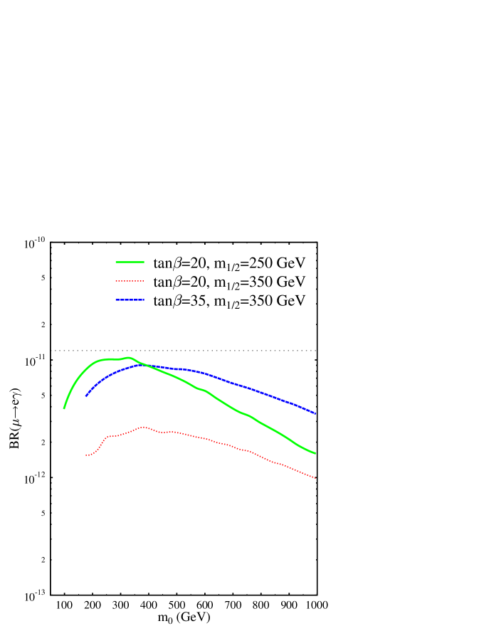
In FIG. 7, we show the branching ratio of $\mu\to e\gamma$ predicted by the above model with $\tan\beta=5,10$. FIG. 8 shows the predicted branching ratio of the model in case of $\tan\beta=20$ and $\tan\beta=35$. In most parameter space in these figures the decay $\mu\to e\gamma$ has a branching ratio close to the present experimental limit and can be easily discovered by the future experiments.

V conclusion and discussion

In this work, we calculate the branching ratio of $\mu\to e\gamma$ in the neutrino mass models with “lopsided” texture of the charged lepton mass matrix, within the supersymmetric framework. The constraints set on the supersymmetric parameter space by the muon anomalous magnetic moment are considered. If the charged lepton mass matrix has symmetric elements between the $1-2$ and $1-3$ generations, this kind of models will generally predict a much larger branching ratio of $\mu\to e\gamma$ than the present experimental limit in most SUSY parameter space.

To accommodate the experimental data, strong constraint should be satisfied by the charged lepton mass matrix, i.e., $({V_{D}})_{13}\lesssim 0.01$. We then show a new kind of models with asymmetric elements between the $1-3$ generations, in addition to the asymmetry between the $2-3$ generations in the “lopsided” models. The large $1-3$ element of the charged lepton mass matrix can suppress $({V_{D}})_{13}$ and at the same time predict a large mixing between the $1-2$ generations naturally. This feature is most interesting in constructing the LMA solution to the solar neutrino problem, which is usually hard to be achieved in the literaturebarr .

With the improvement of the sensitivity to the LFV processes by three or more orders in the next generation experimentsnexp , it is quite possible that the LFV processes will be discovered in the near future. $\tau\to\mu\gamma$ is a promising process to determine whether there is a large mixing between the $2-3$ generations in the charged lepton sector, such as in the “lopsided” modelsbi . If both $\tau\to\mu\gamma$ and $\mu\to e\gamma$ are discovered in the near future, a kind of lepton structure as given by the present work should be very attractive. If only $\tau\to\mu\gamma$ is found, this will imply a large mixing between the $2-3$ generations in the charged lepton sector. However, very special structure should be designed to suppress the $\mu\to e\gamma$ process further. On the contrary, if $\tau\to\mu\gamma$ is not found while $\mu\to e\gamma$ is found, this should be easy to understand and in most models without a lopsided structure this case is predicted. The last possibility is that no LFV is found at all. In this case the most natural explanation is that the soft-SUSY breaking parameters are universal at the energy scale not much higher than the weak scale, such as in the GMSB mechanism.

If LFV is found in the near future, the particles inducing LFV, such as the SUSY particles, may be produced directly on the high energy colliders. The measurements on high energy colliders will help us to infer the flavor structure when combining with the LFV experimental results. At the same time, interplay with the experiments of neutrino oscillation is important. If LFV is found and at the same time $U_{e3}$ of the MNS matrix is measured, much more constraint is obtained in building the neutrino mass models. In any case, the measurement of lepton flavor violation is quite important to infer the possible lepton flavor structure or other possible new physics, no matter the result is positive or null.