Chirally symmetric quark description of low energy $\pi-\pi$ scattering

Abstract

Weinberg’s theorem for $\pi-\pi$ scattering, including the Adler zero at threshold in the chiral limit, is analytically proved for microscopic quark models that preserve chiral symmetry. Implementing Ward–Takahashi identities, the isospin $0$ and $2$ scattering lengths are derived in exact agreement with Weinberg’s low energy results. Our proof applies to alternative quark formulations including the Hamiltonian and Euclidean space Dyson–Schwinger approaches. Finally, the threshold $\pi-\pi$ scattering amplitudes are calculated using the Dyson–Schwinger equations in the rainbow-ladder truncation, confirming the formal derivation.

Pacs Numbers: 11.30.Rd, 14.40.Aq, 12.38.Lg, 12.39.Pn, 11.10.St, 24.85.+p

I Introduction

In the zero quark mass limit the strong interaction is chirally symmetric, exhibiting invariance under independent rotations of left and right handed flavors. Nonvanishing, albeit small on the hadronic scale, $u$ and $d$ quark masses explicitly break this symmetry. More importantly, however, chiral symmetry is also broken spontaneously by the vacuum and the corresponding Goldstone boson is the pion. Thus, it is generally accepted that chiral symmetry underlines the dynamics of soft pions. In particular, the low energy $\pi-\pi$ scattering lengths can be calculated using current algebra and PCAC. In the seminal paper, based on these constraints, Weinberg [1] deduced the scattering lengths for total isospin 0 and 2 to be $a_{0}=+7L/4$ and $a_{2}=-L/2$, respectively, where $L=m^{2}_{\pi}/(8\pi f^{2}_{\pi})$ is given in terms of the pion mass, $m_{\pi}$, and decay constant, $f_{\pi}$. Further, chiral symmetry can also be used to constrain low energy, effective theories describing pion-hadron interactions. For example in the linear $\sigma$ model, chiral symmetry enforces delicate cancellations between direct $\pi-\pi$ interactions and $\sigma$-exchange contributions to the scattering amplitude.

Concurrently, the advent of QCD has spawned the development of more fundamental, microscopic formulations with quark degrees of freedom and low energy hadronic phenomena has been successfully described by various constituent quark models. However, because constituent quark models generally do not respect chiral symmetry, the Goldstone nature of the pion is lost and there is no fundamental difference between pion and, for example, the $\rho$ meson. Consequently, such models should not be expected to properly describe low energy pion scattering.

It is, however, possible to construct quark models implementing chiral symmetry, such as the rainbow-ladder truncation of the set of Dyson–Schwinger equations [DSE] and the instantaneous Hamiltonian approach using the random phase approximation [RPA], which preserve the pion’s Goldstone nature. For such models it is remarkable that both calculated observables and attending mathematical relationships governed by chiral symmetry are largely model independent, even though gauge dependent nonobservable constructs, such as quark and gluon propagators, can be very model sensitive. The pion mass is a quintessential example since for massless quarks this mass is zero, regardless of the form of the effective interaction provided that there is spontaneous dynamical chiral symmetry breaking ($S\chi SB$). Similarly, $\pi$-$\pi$ scattering near threshold is governed by this symmetry and any model that preserves chirality should reproduce Weinberg’s scattering lengths.

The purpose of this paper is to demonstrate that for a microscopic quark formulation with an arbitrary, but chiral symmetry preserving, quark-antiquark interaction Weinberg’s results can indeed be explicitly obtained, and that a correct description of low-energy $\pi$-$\pi$ scattering emerges. The crucial step is to realize that there are important higher order contributions to $\pi$-$\pi$ scattering which, in the chiral limit, must exactly cancel the impulse contribution to recover the Adler zero. Similar effects occur in the microscopic Nambu–Jona-Lasinio model with contact interactions at the quark level [2]. This is closely related to the above mentioned cancellation in the $\sigma$ model. The same results can also be derived in models using bosonization techniques for the chiral pion fields as demonstrated in Ref. [3].

This paper is organized into five sections. In section II we utilize the Hamiltonian formulation to succintly derive Weinberg’s results for the special case of an infinite interaction. Sections III and IV detail the more general proof but now using the rainbow-ladder truncation of the DSE. We also demonstrate the direct contribution to $\pi-\pi$ scattering violates chiral symmetry (does not vanish in the chiral limit) using the axial-vector Ward–Takahashi identity [AV-WTI] and provide a numerical solution of the DSE further documenting the agreement with Weinberg’s scattering lengths. Finally, results and conclusions are summarized in Sec. V.

II Hamiltonian description of $\pi-\pi$ scattering

In this section we provide a synopsis of our key result within the Hamiltonian framework. In section II.A we first address the one pion system and $S\chi SB$. Then in the following subsection we derive Weinberg’s $\pi-\pi$ result in the infinite interaction limit.

A Single pion formulation and $S\chi SB$

The Hamiltonian formalism for pions has an established history. For an earlier reference consult Ref. [4] along with Refs. [5, 6, 7, 8] for more recent applications. In the Hilbert space of pion Salpeter amplitudes the Hamiltonian can be expressed as

$$H=\sigma_{3}\ \left[\begin{array}[]{c}\Phi^{+}\\ \Phi^{-}\end{array}\right]\ m_{\pi}\ [\Phi^{+},\Phi^{-}]\ \sigma_{3}+\sigma_{3}\ \left[\begin{array}[]{c}\Phi^{-}\\ \Phi^{+}\end{array}\right]\ m_{\pi}\ [\Phi^{-},\Phi^{+}]\ \sigma_{3}$$ (1)

with

$$H\ \left[\begin{array}[]{c}\Phi^{+}\\ \Phi^{-}\end{array}\right]=m_{\pi}\ \sigma_{3}\ \left[\begin{array}[]{c}\Phi^{+}\\ \Phi^{-}\end{array}\right];\ H\ \left[\begin{array}[]{c}\Phi^{-}\\ \Phi^{+}\end{array}\right]=-m_{\pi}\ \sigma_{3}\ \left[\begin{array}[]{c}\Phi^{-}\\ \Phi^{+}\end{array}\right].$$ (2)

The normalization is given by

$$\int d^{3}k[\Phi^{+},\Phi^{-}]\ \sigma_{3}\ \left[\begin{array}[]{c}\Phi^{+}\\ \Phi^{-}\end{array}\right]=1$$ (3)

where $\sigma_{3}$ is the standard third component Pauli matrix and $\Phi^{+},\Phi^{-}$ represents the pion positive, negative energy components, respectively. For $\Phi^{+}\rightarrow\Phi^{-}$, $m_{\pi}\rightarrow-m_{\pi}$ while for $\Phi^{+}=\Phi^{-}$, $m_{\pi}=0$.

Previous pion Hamiltonian studies [5, 6, 7, 8] have utilized the Bogolubov-Valatin [BV] (or Bardeen, Cooper, Schriffer [BCS]) transformation approach to describe the ground state vacuum and developed quasiparticle (rotated quark/anti-quark creation and annilhilation) operators for describing the pion in the random phase approximation RPA [7, 8]. The RPA Hamiltonian formalism rigorously preserves chiral symmetry and is formally equivalent to the rainbow-ladder DSE, Bethe–Salpeter equation [BSE] approach with an instantaneous kernel provided the quark propagator is consistent with the BCS vacuum. As detailed elsewhere [9] the pion momentum wavefunction can be expressed in terms of the BV rotation (or BCS gap) angle $\phi(k)$

$$\Phi^{\pm}=\frac{\sin(\phi)}{a}\pm a\ \Delta;\ \;\;a=\sqrt{\frac{2}{3}}\ f_{\pi}\ \sqrt{m_{\pi}}\ .$$ (4)

For $m_{\pi}=0$, $\Delta=0$ and the rest frame pion Salpeter amplitudes reduce to $\Phi^{\pm}=\sin(\phi)/(0)$ which are degenerate and non-normalizable.

The derivation of the above equations follows straightforwardly from an instantaneous reduction of the pion Dyson–Schwinger, Bethe–Salpeter equation which is depicted in Fig. 1. References [9, 10, 11] contain a more complete derivation along with applications. In this formulation the mechanism of spontaneous chiral symmetry breaking is simple to understand: it corresponds to a self-consistent choice of the fermion Fock space appropriate to the quark kernel in use. The Pauli principle still permits an infinite set of Fock spaces which can be isomorphically mapped to an infinite set of functions with coordinates $\phi(k)$. Any such Fock space can be obtained from the trivial one by a BV transformation with a $\phi(k)$ that is determined by solving the mass gap equation. This in turn specifies the physical Fock space. For further information, including the origin of $\phi$, consult Refs. [5, 6, 7, 8].

FIG. 1.: Pion Salpeter equation. In terms of the Dirac matrices $\beta$ and $\vec{\alpha}$, the projection operators for the quark propagator, with momentum $\vec{k}$, are $\Lambda^{\pm}=(1\pm\sin(\phi)\beta\pm\cos(\phi){\bf\alpha}\cdot\widehat{{\bf k}})/2$, and denoted in the figure by $\{+,-\}$. Note that $\Phi^{\pm}$ is consistent with the normalization condition, Eq. (3), and should contain the cluster propagators obtained after integrating the quark propagator energy, $E_{q}$. This is the reason the propagator cuts are displayed in the figure. Two such cluster propagators are needed for the two $\Phi$’ s but only one is generated per integration loop. This necessitates multiplying and dividing the diagrams by the missing cluster propagator leading to the factors $\pm m_{\pi}+E_{q}+E_{\bar{q}}$ appearing in the diagram.

B $\pi-\pi$ scattering

For $\ \pi-\pi$ scattering we can repeat the steps represented in Fig. 1. This is diagrammatically summarized in Fig. 2. Here $\{1,2\}$ represent the incoming pions while $\{3,4\}$ denote the outgoing particles. Both the initial and final configurations now have two energy-spin Salpeter amplitudes. In total there are 48 diagrams plus kinetic energy insertions. The $\pm$ superscripts for pions 1…4 represent the different energy-spin amplitudes. Notice that these diagrams closely resemble those of Fig. 1 so that we could anticipate the model independence of $\pi-\pi$ scattering lengths since the map $\{\pi\times\pi\rightarrow\pi\}$ respects the structure of the pion Salpeter equation [12].

FIG. 2.: Representative $\pi\ -\pi$ scattering diagrams.

Figure 2 clearly indicates that both quark exchange and quark annihilation amplitudes are necessary. Of course this is a consequence of the quark Dirac nature, however, it is important to note that with just quark exchange only repulsion is obtained. This is precisely the case of exotic scattering. It is chiral symmetry which governs the correct combination of exchange and annihilation diagrams to yield a Goldstone pion and by doing so, to produce the Weinberg scattering lengths.

We now evaluate the isospin $I=0$ and $2$ $\pi-\pi$ $T$ matrix, $T_{I}$, or scattering amplitude $A_{I}=i4\pi m_{\pi}T_{I}$, at zero pion momentum. Either from comparing Figs. 1 and 2 or from Eqs. (1), (2) and (3) it is clear that $T_{I}$ will be proportional to $m_{\pi}$ because H is proportional to $m_{\pi}$. Further, $T_{I}$ is also inversely proportional to $f_{\pi}$ since there are just two extra pion amplitudes when going from the Salpeter equation for one single pion to $\pi-\pi$ scattering. After including all potential energy diagrams plus kinetic insertions we have,

$$T_{I}=b_{I}\left[{\Phi^{-}}^{2},{\Phi^{+}}^{2}\right]H\left[\begin{array}[]{c}{\Phi^{+}}^{2}\\ {\Phi^{-}}^{2}\end{array}\right]+c_{I}\left[\Phi^{+}\Phi^{-},\Phi^{+}\Phi^{-}\right]H\left[\begin{array}[]{c}\Phi^{+}\Phi^{-}\\ \Phi^{-}\Phi^{-}\end{array}\right]+d_{I}\left[{\Phi^{+}}^{2},{\Phi^{-}}^{2}\right]H\left[\begin{array}[]{c}{\Phi^{+}}^{2}\\ {\Phi^{-}}^{2}\end{array}\right]\ .$$ (5)

In the above expression integration is assumed. The Hamiltonian is given by Eq. (2) and the constants, entailing color, spin and isospin traces, are

$$b_{[I=0,I=2]}=\left[3/4,0\right];\;c_{[0,2]}=\left[3/4,0\right];\;d_{[0,2]}=\left[-1/2,1\right]\ .$$ (6)

Equation (5) is especially simple to evaluate for an infinite interaction since $\sin\phi(k)\rightarrow 1$. This limit always exists because for a given class of the quark kernels (for instance linear confinement with potential $\sigma r$) the mass gap equation for $\phi(k)$ can always be re-scaled as an dimensionless equation for $\phi(k/\sigma)$ for an arbitrary kernel strength $\sigma$. In the extremely strong limit, which also corresponds to the pion point limit, $\sigma\rightarrow\infty$, and $\phi(k/\sigma)\rightarrow\phi(0)=\pi/2$ which is sufficient to obtain Weinberg’s scattering lengths. To appreciate this use Eq.(4) repeatively with $\sin(\phi)=1$ to obtain,

$$\int\left[{\Phi}^{+},{\Phi}^{-}\right]\;\sigma_{3}\;\left[\begin{array}[]{c}\Phi^{+}\\ \Phi^{-}\end{array}\right]=\int 4\sin(\phi)\Delta=1;\;\int\left[\Phi^{-},\Phi^{+}\right]\;\sigma_{3}\;\left[\begin{array}[]{c}{\Phi^{+}}^{2}\\ {\Phi^{-}}^{2}\end{array}\right]=\int 2\sin^{2}(\phi)\Delta=1/2$$ (7)

and so on… It is then a text book calculation to extract, in lowest order in $m_{\pi}$, the $\pi-\pi$ scattering lengths from the $T$ matrix, Eq.(5), since in the Born approximation $a_{I}=m_{\pi}T_{I}/(4\pi)$ and we get the desired result $a_{[0,2]}=[7/4,-1/2]L$.

With this preliminary treatment we now address the more general derivation for an arbitrary but finite quark kernel. First we demonstrate that the impulse approximation is insufficient for $\pi-\pi$ scattering and violates chiral symmetry.

III Impulse approximation for $\pi-\pi$ scattering

In this section we evaluate the leading (box) diagrams for $\pi-\pi$ scattering and demonstrate that they fail to provide a correct description since they violate chiral symmetry. These diagrams, which we call direct terms, correspond to the impulse approximation and are illustrated in Fig. 3.

FIG. 3.: Three different topologies for the direct contribution to $\pi-\pi$ scattering. Reversing the quark and anti-quark flow (reversing the arrow) generates three other diagrams for a total of six. The larger solid cirlces represent the pion-quark vertex while the smaller solid circles denote the quark propagators are dressed.

We can evaluated the direct terms model-independently using the AV-WTI which exactly relates the axial-vector, $\Gamma_{\mu}^{5}$, and pseudoscalar, $\Gamma^{5}$, vertices to the inverse of the dressed quark propagator

$$-i\left(P^{\mu}\Gamma_{\mu}^{5}(p^{\prime},p;P)-2\,m_{q}(\mu)\,\Gamma^{5}(p^{\prime},p;P)\right) = S^{-1}(p^{\prime})\gamma_{5}+\gamma_{5}S^{-1}(p)\,.$$ (8)

Here $p$, $p^{\prime}=p+P$ are the respective incoming, outgoing quark momenta, and $P$ the momentum flowing into the vertex. The inverse of the dressed quark propagator, $S^{-1}(p)$, can be expressed in terms of scalar functions $A$ and $B$

$$iS^{-1}(p) = \,A(p^{2})\;p\!\!\!/-B(p^{2})\,.$$ (9)

For the free propagator $A=1$ and $B=m_{q}(\mu)$, the current quark mass which explicitly breaks chiral symmetry. Since the interaction contains a diverging, but renormalizable, short-range component, this mass requires renormalization and depends on scale $\mu$.

Meson bound states can be described by a Bethe–Salpeter amplitude [BSA] satisfying a homogeneous BSE

$$\Gamma^{ab}_{H}(p^{\prime},p;P) = \int_{k}K^{ab;cd}(p^{\prime},p;k,k^{\prime})\;\left[S(k^{\prime})\,\Gamma_{H}(k^{\prime},k;P)\,S(k)\right]^{dc}\,,$$ (10)

with $\int_{k}$ representing $\int\frac{d^{4}k}{(2\pi)^{4}}$ and $K$ is the quark-antiquark scattering kernel, properly regularized for divergent integrals. This equation only has solutions for discrete values of $P^{2}$ corresponding to the bound state mass. The lowest bound state in the pseudoscalar channel is the pion, $P^{2}=M^{2}_{\pi}$, which produces poles in both $\Gamma_{\mu}^{5}$ and $\Gamma^{5}$. For the axial-vector vertex the residue of this pole is $f_{\pi}P_{\mu}$, while the residue of pseudoscalar vertex is labeled $r_{P}(\mu)$. Both can be calculated from the properly normalized pion BSA and the dressed quark propagators

$$P_{\mu}\,f_{\pi} = i\,Z_{2}\int_{k}{\rm Tr}\left[S(k^{\prime})\;\Gamma_{\pi}(k^{\prime},k;P)\;S(k)\;\gamma_{\mu}\gamma_{5}\right]\,,$$ (11)

$$m_{q}(\mu)\;r_{P}(\mu) = -Z_{4}\,m_{q}(\mu)\,\int_{k}{\rm Tr}\left[S(k^{\prime})\;\Gamma_{\pi}(k^{\prime},k;P)\;S(k)\;\gamma_{5}\right]\,.$$ (12)

The constants $Z_{2}$ and $Z_{4}$ are the usual quark wave function and mass renormalization terms, respectively. They depend on both renormalization and regulator scales but when combined with the integrals and $m_{q}(\mu)$ incorporated in the above expressions, the final results are scale independent [13]. This has been checked explicitly for a model having an effective interaction that reduces to the one-loop running coupling [14]. Finally, these residues are constrained to cancel through the AV-WTI

$$M^{2}_{\pi}\,f_{\pi}-2\;m_{q}(\mu)\;r_{P}(\mu) = 0\,.$$ (13)

Even though there is no pion pole in the inverse quark propagator, we can still use the AV-WTI to express $\Gamma_{\pi}$ in terms of the inverse quark propagator. In the combined chiral and $P_{\mu}\rightarrow 0$ limit this yields

$$\Gamma_{\pi}(p,p;0) = \frac{B_{0}(p^{2})}{f_{\pi}}\gamma_{5}$$ (14)

where the subscript 0 indicates the chiral limit.

The evaluation of the direct terms in Fig. 3 produces

$$\int_{k}{\rm Tr}[\Gamma_{\pi}(k+P_{1},k;P_{1})\,S(k)\,\Gamma_{\pi}(k,k-P_{2};P_{2})\,S(k-P_{2})\bar{\Gamma}_{\pi}(k-P_{2},k-P_{2}-P_{3};P_{3})\,$$ (15)

$${}\times S(k-P_{2}-P_{3})\,\bar{\Gamma}_{\pi}(k-P_{2}-P_{3},k+P_{1};P_{4})\,S(k+P_{1})]\;,$$ (16)

which at threshold and along with Eq. (14), reduces in the chiral limit to

$$\frac{1}{f_{\pi}^{4}}\int_{k}\frac{B_{0}^{4}(k)}{(k^{2}A_{0}^{2}(k)+B_{0}^{2}(k))^{2}} \neq 0\;.$$ (17)

Note that this direct term result, which is exact since it follows from the AV-WTI, is not zero in the chiral limit. From Weinberg’s theorem, however, the $\pi-\pi$ scattering amplitude at threshold scales as $M^{2}_{\pi}/{f^{2}_{\pi}}$ and therefore must vanish in the chiral limit. Clearly the direct term alone is insufficient to obtain Weinberg’s result and additional diagrams are necessary.

IV Dyson–Schwinger in the Rainbow-Ladder Approach

The problem raised in the previous section can be resolved by utilizing a formalism which preserves chiral symmetry. In this section we consider one such approach, the Dyson–Schwinger method in the rainbow ladder truncation (see Ref.[15] for a review and applications). The set of DSEs form a hierarchy of coupled integral equations for the Green’s function of the underlying theory. For example, the quark propagator $S(p)$ satisfies

$$iS^{-1}(p) = Z_{2}\;p\!\!\!/-Z_{4}\,m_{q}(\mu)-i\int_{k}g^{2}\;\gamma_{\mu}\frac{\lambda^{i}}{2}\;S(k)\;\Gamma^{i}_{\nu}(k,p)\;D^{\mu\nu}(k-p)\,,$$ (18)

where $\Gamma^{i}_{\nu}(k,p)$ is the dressed quark-gluon vertex with gluon color label $i=1\ldots 8$ and $D^{\mu\nu}(k-p)$ is the gluon propagator. The constants $Z_{2}$ and $Z_{4}$ follow from the renormalization condition

$$iS^{-1}(p)\Big{|}_{p^{2}=\mu^{2}} = p\!\!\!/-m_{q}(\mu)$$ (19)

at the renormalization scale $\mu$. The equation for the axial-vector vertex $\Gamma_{\mu}^{5}(p^{\prime},p;P)$ and the pseudoscalar vertex $\Gamma^{5}(p^{\prime},p;P)$ is the generic inhomogeneous BSE

$$\Gamma^{ab}(p^{\prime},p;P) = \gamma_{\hbox{inhom}}+\int_{k}K^{ab;cd}(p^{\prime},p;k,k^{\prime})\;\left[S(k^{\prime})\,\Gamma(k^{\prime},k;P)\,S(k)\right]^{dc}\,,$$ (20)

with the inhomogeneous terms $Z_{2}\,\gamma_{\mu}\,\gamma^{5}$ and $Z_{4}\,\gamma^{5}$, respectively. It is convenient to define an axial vertex $\Gamma_{A}$

$$\Gamma_{A}(p^{\prime},p;P) = -i\left(P^{\mu}\Gamma_{\mu}^{5}(p^{\prime},p;P)-2\,m_{q}(\mu)\,\Gamma^{5}(p^{\prime},p;P)\right)\,,$$ (21)

which satisfies the BSE with inhomogeneous term

$$\gamma_{A}(P) = -i\left(Z_{2}\,P\!\!\!\!/\,-2\,Z_{4}\,m_{q}(\mu)\right)\gamma^{5}\,.$$ (22)

For this vertex, the AV-WTI reduces to

$$\Gamma_{A}(p^{\prime},p;P) = S^{-1}(p^{\prime})\gamma_{5}+\gamma_{5}S^{-1}(p)\,.$$ (23)

From Eqs. (11)-(13) it follows that for any four-momentum $Q$ flowing into the diagram we have

$$\int_{k}{\rm Tr}\left[S(k+P)\;\Gamma_{\pi}(k+P,k;P)\;S(k)\;\gamma_{A}(Q)\right] = (P\cdot Q+M^{2}_{\pi})\,f_{\pi}\,.$$ (24)

Finally, expanding the vertex in powers of $P$, valid for low momentum, small quark and pion masses, yields

$$\frac{i}{2\;f_{\pi}}\Gamma_{A}(p^{\prime},p;P) = \Gamma_{\pi}(p^{\prime},p;P)+{\cal O}(P)+{\cal O}(m_{q}(\mu))\,.$$ (25)

A Rainbow-ladder truncation

Provided that the regularization scheme is translationally invariant, the rainbow truncation for the quark DSE

$$iS^{-1}(p) = Z_{2}\;p\!\!\!/-Z_{4}\,m_{q}(\mu)-i\int_{k}\gamma_{\mu}\frac{\lambda^{i}}{2}\;S(k)\;\gamma_{\nu}\frac{\lambda^{i}}{2}\;g^{2}D^{\mu\nu}(k-p)\,,$$ (26)

combined with the ladder truncation for the quark-antiquark scattering kernel

$$K^{ab;cd}(p^{\prime},p;k,k^{\prime}) = \gamma_{\mu}^{ad}\frac{\lambda^{i}}{2}\;\gamma_{\nu}^{cb}\frac{\lambda^{i}}{2}\;g^{2}D^{\mu\nu}(p-k)\,,$$ (27)

is consistent with the Ward identities[14, 16]. To discuss $\pi-\pi$ scattering, we introduce the unamputated quark-antiquark scattering amplitude, $L$, in the ladder truncation which is pictorially represented in Fig. 4. Here the solid horizontal lines represent quark (antiquark) propagation and the coiled vertical lines correspond to the quark-antiquark kernel, $K$, in the ladder truncation, Eq. (27).

FIG. 4.: The unamputated quark-antiquark scattering amplitude $L$ in the ladder truncation. The quark propagators are dressed, but for simplicity the solid circles indicating the dressing are omitted in this and subsequent diagrams.

This scattering amplitude satisfies the following DSE in the ladder truncation

$$L^{ab;cd}(p^{\prime},p;k,k^{\prime}) = S^{ad}(p)\;S^{cb}(k)\;\delta^{4}(p-k)$$ (29)

$${}-\int_{q}S^{aa^{\prime}}(p^{\prime})\,\gamma_{\mu}^{a^{\prime}d^{\prime}}\,L^{d^{\prime}c^{\prime};cd}(q^{\prime},q;k,k^{\prime})\,\gamma_{\nu}^{c^{\prime}b^{\prime}}\,S^{b^{\prime}b}(p)\,g^{2}D^{\mu\nu}(p-q)\;.$$

Using the AV-WTI, the ladder truncated amplitudes connected by the vertex $\Gamma_{A}$, depicted in Fig. 5, can be reduced to (see Ref.[11] for a similar reduction of the vector vertex)

$$\int_{q}L^{ab;b^{\prime}a^{\prime}}(p^{\prime}+Q,p;q,q^{\prime}+Q)\;\Gamma_{A}^{a^{\prime}d^{\prime}}(q^{\prime}+Q,q^{\prime};Q)\;L^{d^{\prime}c^{\prime};cd}(q^{\prime},q;k,k^{\prime})\;(S^{-1})^{c^{\prime}b^{\prime}}(q)$$ (30)

$$= \gamma_{5}^{aa^{\prime}}\;L^{a^{\prime}b;cd}(p^{\prime},p;k,k^{\prime})+L^{ab;cd^{\prime}}(p^{\prime}+Q,p;k,k^{\prime})\;\gamma_{5}^{d^{\prime}d}\,.$$ (31)

FIG. 5.: Reduction of connected ladder amplitudes.

Related, it can also be shown in the combined rainbow-ladder truncation that

$$\int_{k}L^{ab;cd}(p+P_{1},p-P_{2};k-P_{2},k+P_{1})\;\left[\Gamma_{A}(k+P_{1},k;P_{1})\;S(k)\;\Gamma_{A}(k,k-P_{2};P_{2})\right]^{dc}$$ (32)

$$= \left[\gamma_{5}\,S(p)\,\Gamma_{A}(p,p-P_{2};P_{2})\,S(p-P_{2})\right]^{ab}+\int_{k}L^{ab;cd}(p+P_{1},p-P_{2};k-P_{2},k+P1)\;\left[\gamma_{5}\;\gamma_{A}(P_{2})\right]^{dc}$$ (33)

and similarly, for on-shell pions

$$\int_{k}L^{ab;cd}(p+P_{1},p-P_{2};k-P_{2},k+P_{1})\;\left[\Gamma_{A}(k+P_{1},k;P_{1})\;S(k)\;\Gamma_{\pi}(k,k-P_{2};P_{2})\right]^{dc}$$ (34)

$${}=\left[\gamma_{5}\,S(p)\,\Gamma_{\pi}(p,p-P_{2};P_{2})\,S(p-P_{2})\right]^{ab}\,.$$ (35)

B $\pi-\pi$ scattering in rainbow-ladder truncation

We now utilize Eq. (25) to evaluate the $\pi-\pi$ scattering amplitude near threshold. Since there are six topologically different ways to attach the external pion legs to the direct term, we first calculate the contribution from one of these topologies by adding two sets of diagrams with a complete set of ladder kernels $K$ inserted in the direct contribution (see Fig. 6 and Ref.[10] for a additional details).

FIG. 6.: Amplitude for $\pi-\pi$ scattering in rainbow-ladder truncation that reproduces Weinberg’s result. Note the $-$ sign for the direct contribution due to the disconnected term in the amplitude $L$.

Then using the notation introduced in the previous section yields the $\pi-\pi$ scattering amplitude, $A$

$$A\;=\;\int_{k}\int_{p}\left[\bar{\Gamma}_{\pi}(p+P_{3},p;P_{3})\,S(p)\,\bar{\Gamma}_{\pi}(p,p-P_{4};P_{4})\right]^{ba}\;L^{ab;cd}(p-P_{4},p+P_{3};k-P_{2},k+P_{1})\;$$ (36)

$$\times\left[\Gamma_{\pi}(k+P_{1},k;P_{1})\,S(k)\,\Gamma_{\pi}(k,k-P_{2};P_{2})\right]^{dc}$$ (37)

$$+\int_{k}\int_{p}\left[\bar{\Gamma}_{\pi}(p+P_{4},p;P_{4})\,S(p)\Gamma_{\pi}(p,p-P_{1};P_{1})\right]^{dc}\;L^{ab;cd}(p-P_{1},p+P_{4};k+P_{2},k-P_{3})\;$$ (38)

$$\times\left[\Gamma_{\pi}(k+P_{2},k;P_{2})\,S(k)\bar{\Gamma}_{\pi}(k,k-P_{3};P_{3})\right]^{dc}$$ (39)

$$-\int_{k}{\rm Tr}[\Gamma_{\pi}(k+P_{1},k;P_{1})\,S(k)\,\Gamma_{\pi}(k,k-P_{2};P_{2})\,S(k-P_{2})\bar{\Gamma}_{\pi}(k-P_{2},k-P_{2}-P_{3};P_{3})\,S(k-P_{2}-P_{3})$$ (40)

$$\times\bar{\Gamma}_{\pi}(k-P_{2}-P_{3},k+P_{1};P_{4})\,S(k+P_{1})]$$ (41)

where the $P_{i}$ are constrained by momentum conservation, $\sum_{i=1}^{4}P_{i}=0$, and the on-shell condition, $P_{i}^{2}=m_{\pi}^{2}$. Note that there is a minus sign for the direct term because our definition of $L$ includes the disconnected contribution (see Eq. (29)). Using the expansion Eq. (25) and the relations Eqs. (24) and (31)-(35), one can show that to order $P_{i}\,P_{j}$ the sum of these diagrams reduces to

$$A = \frac{i}{4f_{\pi}^{2}}\left((P_{1}+P_{2})^{2}+(P_{1}+P_{4})^{2}-2m_{\pi}^{2}\right)\,.$$ (42)

It immediately follows that the $\pi-\pi$ scattering amplitude at threshold is proportional $(m_{\pi}/{f_{\pi}})^{2}$ and vanishes for $m_{\pi}\rightarrow 0$. This is the Adler zero. Hence, in the chiral limit the sum of the ladder diagrams exactly cancels the direct term contribution.

For the physical scattering amplitude all six topologies must be added, each with the appropriate combination of isospin factors. In terms of the usual Mandelstam variables, $s$, $t$ and $u$, the final result is

$$A_{0} = i\,{2\,s-m_{\pi}^{2}\over 2f_{\pi}^{2}}\ ,$$ (43)

for the $I=0$ amplitude, and

$$A_{2} = i\,{-\,s+2m_{\pi}^{2}\over 2f_{\pi}^{2}}\ ,$$ (44)

for the $I=2$ amplitude, respectively. This reduces to the Weinberg limit at threshold ($s=4m^{2}_{\pi}$)

$$A_{0} = i\,{7m_{\pi}^{2}\over 2f_{\pi}^{2}}=i\,16\,\pi\,a_{0}\ ,$$ (45)

$$A_{2} = -i\,{m_{\pi}^{2}\over f_{\pi}^{2}}=i\,16\,\pi\,a_{2}\ ,$$ (46)

independent of ladder kernel details. Here $a_{I}$ are the S wave scattering lengths. Hence, to properly describe $\pi-\pi$ scattering in the rainbow-ladder truncation, all possible diagrams with one or more insertions of the ladder kernel $K$ must be combined with the direct terms. Note that for the direct terms there is implicitly an infinite number of ladders inserted “across one BSA in a corner” and on the bare quark lines. Thus, for a consistent calculation, the ladder kernel must be inserted, in all possible ways, without crossing, in the skeleton diagrams like the ones in Fig. 3. This prescription can easily be generalized to other processes even if they involve a different number of external particles. In particular for processes with three external particles, the impulse approximation in combination with the rainbow-ladder truncation for the quark propagators and vertices does satisfy consistency requirements following from current conservation (see Ref.[18] for an electromagnetic application). In this case all possible insertions of the ladder kernel (without crossing) are already implicitly included in the dressing of the propagators and vertices.

C Numerical results at threshold

Utilizing the DSE model and calculation scheme of Refs. [17, 18], we have conducted a numerical analysis of $\pi-\pi$ scattering. Figure 7 shows our results for both isospin scattering amplitudes at threshold as a function of the current quark mass (the imaginary phase has been suppressed). The corresponding pion mass and decay constant are also calculated as a function of the quark mass and the square of their ratio is plotted as well. This model calculation clearly shows that the scattering amplitudes indeed behave like $M^{2}_{\pi}/f_{\pi}^{2}$ if one includes the two complete sets of ladder diagrams in addition to the direct term, as indicated in Fig. 6. In the chiral limit the two sets of ladders cancel the direct contribution within the numerical accuracy.

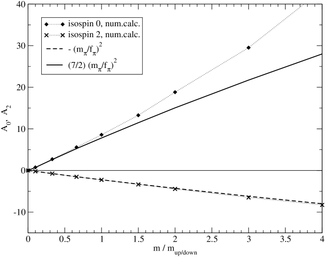
FIG. 7.: The $\pi-\pi$ scattering amplitudes at threshold calculated in rainbow-ladder truncation as a function of the current quark mass. For comparison, we also show the Weinberg limit, using our calculated values for $m_{\pi}$ and $f_{\pi}$.

It is interesting that the direct term alone generates a scattering amplitude about 20 times larger than observation. For the physical value of the degenerate $u$, $d$ current quark mass, $m_{q}=5.54$ $MeV$ at renormalization scale $\mu=1$ $GeV$, about 95% of the direct contribution is cancelled by including the ladder diagrams. For this quark mass our corresponding scattering lengths are $a_{0}=0.170$ and $a_{2}=-0.045$ which again are in excellent agreement with Weinberg’s values of $a_{0}=0.156$ and $a_{2}=-0.044$ (using $m_{\pi}=138.04\,{\rm MeV}$ and $f_{\pi}=92.44\,~{}{\rm MeV}$). This is also in good agreement with the physical $\pi-\pi$ scattering lengths, $a_{0}=0.220$ and $a_{2}=-0.0444$.

It is also interesting to note that chiral perturbation theory reproduces even more precisely the physical scattering lengths [19]. This is due to pion loops, which we have not included, and the isospin $0$ channel is more sensitive than the isospin $2$ channel to this effect. The 3rd order chiral perturbation theory for $a_{2}$ is almost identical to Weinberg’s value, whereas there are significant corrections from 2nd and even 3rd order chiral perturbation theory to Weinberg’s $a_{0}$.

In addition to chiral symmetry there is another important correction that is implicitly included in our approach. This is the effect from scalar bound states. In particular an idealized $\sigma$ meson, which appears as a $q\bar{q}$ bound state in our model, is present and also influences the isospin zero scattering amplitude.

V Further comments and conclusion

Summarizing, we find chiral symmetry preserving quark models can indeed yield the correct $I=0$ and $I=2$ $\pi-\pi$ scattering amplitudes near threshold, $(2s-m_{\pi}^{2})/(2i\,f_{\pi}^{2})$ and $(-s+2m_{\pi}^{2})/(2i\,f_{\pi}^{2})$, respectively. Further, we have rigorously reproduced Weinberg’s low energy theorem for the scattering lengths. We have proved this independent of the interaction details for a manifestly covariant DSE/BSE approach using the rainbow-ladder truncation, and also for an instantaneous Hamiltonian formulation in the infinite interaction limit. In the former case this result has also been demonstrated by summing the series of diagrams in Fig. 6 numerically using the model of Ref. [17, 18]. Lastly, both approaches produce the Adler zero which provides new and important bounds for couplings to scalar mesons.

We expect our result to be a general feature in any quark model preserving both chiral symmetry and the AV-WTI. However, care is necessary to ensure any truncation does indeed satisfy all chiral symmetry constraints. For ladder truncations, the crucial step is to include all diagrams with the ladder kernel inserted in the direct contribution. Finally, we submit this prescription is also necessary for consistency in other processes (e.g. current conservation), as well as reactions involving more than four external particles.

REFERENCES

- [1] S. Weinberg, Phys. Rev. Lett. 17, 616 (1966).
- [2] V. Bernard, U. G. Meissner, A. Blin, and B. Hiller, Phys. Lett. B253, 443 (1991); V. Bernard, A. H. Blin, B. Hiller, Y. P. Ivanov, A. A. Osipov, and U. Meissner, Annals Phys. 249, 499 (1996).
- [3] C. D. Roberts, R. T. Cahill, M. E. Sevior, and N. Iannella, Phys. Rev. D 49, 125 (1994).
- [4] J. D. Bjorken and S. D. Drell, Relativistic Quantum Mechanics, Chapter 9.7 (Mcgraw-Hill, 1964).
- [5] P. Bicudo and J. Ribeiro, Phys. Rev. D 42, 1611 (1990).
- [6] P. Bicudo, G. Krein, J. Ribeiro, and J. Villate, Phys. Rev. D 45, 1673 (1992).
- [7] F. J. Llanes-Estrada and S. R. Cotanch, Phys. Rev. Lett. 84, 1102 (2000).
- [8] F. J. Llanes-Estrada and S. R. Cotanch, Nucl. Phys. A697, 303 (2002).
- [9] A. Le Yaouanc, L. Oliver, O. Péne, and J.-C. Raynal, Phys. Rev. D 31, 137 (1985); P. Bicudo and J. Ribeiro, Phys. Rev. D 42, 1625 (1990).
- [10] P. Bicudo and J. Ribeiro, Phys. Rev. D 42, 1635 (1990).
- [11] P. Bicudo, Phys. Rev. C 60, 035209 (1999).
- [12] J. Ribeiro, Quark Confinement and the Hadron spectrum IV (World Scientific, in press).
- [13] P. Maris, C. D. Roberts, and P. C. Tandy, Phys. Lett. B 420, 267 (1998).
- [14] P. Maris and C. D. Roberts, Phys. Rev. C 56, 3369 (1997).
- [15] C. D. Roberts and A. G. Williams, Prog. Part. Nucl. Phys. 33, 477 (1994); R. Alkofer and L. von Smekal, Phys. Rept. 353, 281 (2001).
- [16] R. Delbourgo and M. D. Scadron, J. Phys. G 5, 1621 (1979).
- [17] P. Maris and P. C. Tandy, Phys. Rev. C 60, 055214 (1999).
- [18] P. Maris and P. C. Tandy, Phys. Rev. C 61, 045202 (2000).
- [19] G. Colangelo, J. Gasser, and H. Leutwyler, Phys. Lett. B488, 261 (2000).