Chapter 1 $B$ Phenomenology

Sheldon Stone
Department of Physics

Syracuse University, USA, 13244-1130

Email: Stone@physics.syr.edu

ABSTRACT

Many topics are discussed in $b$ physics including lifetimes, decay mechanisms, determinations of the CKM matrix elements $|V_{cb}|$ and $|V_{ub}|$, facilities for $b$ quark studies, neutral $B$ meson mixing, rare $b$ decays, hadronic decays and CP violation. I review techniques for finding physics beyond the Standard Model and describe the complimentarity of $b$ decay measurements in elucidating new physics that could be found at higher energy machines.

..

Lectures presented at 55th Scottish Universities Summer School in Physics on Heavy Flavour Physics, A NATO Advanced Study Insititute, St. Andrews, Scotland, August, 2001.

Contents

1. 1 $B$ Phenomenology
   1. 1 Introduction: The Standard Model and $B$ Decays
      1. 1.1 Theoretical Basis
      2. 1.2 Lifetime Measurements
      3. 1.3 $B$ Decay Mechanisms
   2. 2 Semileptonic $B$ Decays
      1. 2.1 Formalism of Exclusive Semileptonic $B$ Decays
      2. 2.2 Measurement of $|V_{cb}|$
      3. 2.3 Measurement of $|V_{ub}|$
   3. 3 Facilities for $b$ Studies
      1. 3.1 $b$ Production Mechanisms
      2. 3.2 Accelerators for $b$ Physics
      3. 3.3 $e^{+}e^{-}$ Detectors
      4. 3.4 $b$ Production Characteristics at Hadron Colliders
   4. 4 $B^{o}-\overline{B}^{o}$ Mixing
      1. 4.1 Introduction
      2. 4.2 $B_{s}$ Mixing in the Standard Model
   5. 5 Rare $b$ Decays
      1. 5.1 Introduction
      2. 5.2 Standard Model Theory
      3. 5.3 $b\to s\gamma$
      4. 5.4 Rare Hadronic Decays
   6. 6 Hadronic Decays
      1. 6.1 Introduction
      2. 6.2 Two-Body Decays into a Charm or Charmonium
      3. 6.3 Observation of the $\rho^{\prime}$ in $B$ Decays
   7. 7 CP Violation
      1. 7.1 Introduction
      2. 7.2 Unitarity Triangles
      3. 7.3 Formalism of CP Violation in Neutral $B$ Decays
      4. 7.4 Results on $\sin{2\beta}$
      5. 7.5 Remarks on Global Fits to CKM parameters
   8. 8 New Physics Studies
      1. 8.1 Introduction
      2. 8.2 Generic Tests for New Physics
      3. 8.3 New Physics Tests in Specific Models
      4. 8.4 Expected Data Samples
   9. 9 Conclusions

1 Introduction: The Standard Model and $B$ Decays

Studies of $b$ and $c$ physics are focused on two main goals. The first is to look for new phenomena beyond the Standard Model. The second is to measure Standard Model parameters including CKM elements and decay constants. These lectures concern “$B$ Phenomenology,” a topic so broad that it can include almost anything concerning $b$ quark decay or production. I will cover an eclectic ensemble of topics that I find interesting and hope will be educational.

1.1 Theoretical Basis

The physical states of the “Standard Model” are comprised of left-handed doublets containing leptons and quarks and right handed singlets (Rosner 2001)

$$\left(\begin{array}[]{c}u\\ d\end{array}\right)_{L}\left(\begin{array}[]{c}c\\ s\end{array}\right)_{L}\left(\begin{array}[]{c}t\\ b\end{array}\right)_{L}, ~{}u_{R},~{}d_{R},~{}c_{R},~{}s_{R},~{}t_{R},~{}b_{R}$$ (7)

$$\left(\begin{array}[]{c}e^{-}\\ \nu_{e}\end{array}\right)_{L}\left(\begin{array}[]{c}\mu^{-}\\ \nu_{\mu}\end{array}\right)_{L}\left(\begin{array}[]{c}\tau^{-}\\ \nu_{\tau}\end{array}\right)_{L}, ~{}e^{-}_{R},~{}\mu^{-}_{R},~{}\tau^{-}_{R},~{}{\nu_{e}}_{R},~{}{\nu_{\mu}}_{R},~{}{\nu_{\tau}}_{R}.$$ (14)

The gauge bosons, $W^{\pm}$, $\gamma$ and $Z^{o}$ couple to mixtures of the physical $d,~{}s$ and $b$ states. This mixing is described by the Cabibbo-Kobayashi-Maskawa (CKM) matrix (see below) (Kobayashi 1973).

The Lagrangian for charged current weak decays is

$$L_{cc}=-{g\over\sqrt{2}}J^{\mu}_{cc}W^{\dagger}_{\mu}+h.c.,$$ (15)

where

$$J^{\mu}_{cc}=\left(\bar{\nu}_{e},~{}\bar{\nu}_{\mu},~{}\bar{\nu}_{\tau}\right)\gamma^{\mu}V_{MNS}\left(\begin{array}[]{c}e_{L}\\ \mu_{L}\\ \tau_{L}\\ \end{array}\right)+\left(\bar{u}_{L},~{}\bar{c}_{L},~{}\bar{t}_{L}\right)\gamma^{\mu}V_{CKM}\left(\begin{array}[]{c}d_{L}\\ s_{L}\\ b_{L}\\ \end{array}\right)$$ (16)

and

$$V_{CKM}=\left(\begin{array}[]{ccc}V_{ud}&V_{us}&V_{ub}\\ V_{cd}&V_{cs}&V_{cb}\\ V_{td}&V_{ts}&V_{tb}\end{array}\right).$$ (17)

Multiplying the mass eigenstates $(d_{L},s_{L},b_{L})$ by the CKM matrix leads to the weak eigenstates. $V_{MNS}$ is the analogous matrix required for massive neutrinos (we will not discuss this matrix any further). There are nine complex CKM elements. These 18 numbers can be reduced to four independent quantities by applying unitarity constraints and the fact that the phases of the quark wave functions are arbitrary. These four remaining numbers are fundamental constants of nature that need to be determined from experiment, like any other fundamental constant such as $\alpha$ or $G$. In the Wolfenstein approximation the matrix is written in order $\lambda^{3}$ for the real part and $\lambda^{4}$ for the imaginary part as (Wolfenstein 1983)

$$V_{CKM}=\left(\begin{array}[]{ccc}1-\lambda^{2}/2&\lambda&A\lambda^{3}(\rho-i\eta)(1-\lambda^{2}/2)\\ -\lambda&1-\lambda^{2}/2-i\eta A^{2}\lambda^{4}&A\lambda^{2}(1+i\eta\lambda^{2})\\ A\lambda^{3}(1-\rho-i\eta)&-A\lambda^{2}&1\end{array}\right).$$ (18)

The constants $\lambda$ and $A$ are determined from charged-current weak decays. The measured values are $\lambda=0.2205\pm 0.0018$ and A=0.784$\pm$0.043. There are constraints on $\rho$ and $\eta$ from other measurements that we will discuss. Usually the matrix is viewed only up to order $\lambda^{3}$. To explain CP violation in the $K^{o}$ system the term of order $\lambda^{4}$ in $V_{cs}$ is necessary.

1.1.1 Determination of $G_{F}$

Muons, being lighter than the lightest hadrons, must decay purely into leptons. The process is $\mu^{-}\to e^{-}\overline{\nu}_{e}\nu_{\mu}$ as shown in Figure 1.

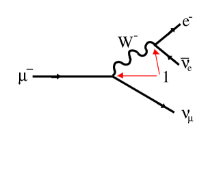
Figure 1: Diagram for muon decay.

The total width for this decay process is given by

$$\Gamma_{\mu}={G_{F}^{2}\over 192\pi^{3}}m^{5}_{\mu}\times{\rm(phase~{}space)}\times{\rm(radiative~{}corrections)}~{}~{}.$$ (19)

Since $\Gamma_{\mu}\cdot\tau_{\mu}=\mbox{$h$\raisebox{-0.04303pt}{${}^{-}$}}$, measuring the muon lifetime gives a direct measure of $G_{F}$.

1.1.2 Determination of $|V_{us}|$

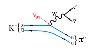
Figure 2: Semileptonic $K^{-}$ decay diagram.

A charged current decay diagram for strange quark decay is shown in Figure 2. Here the CKM element $V_{us}$ is present. The decay rate is given by a formula similar to equation (19), with the muon mass replaced by the $s$-quark mass and an additional factor of $|V_{us}|^{2}$. Two complications arise since we are now measuring a decay process involving hadrons, $K^{-}\to\pi^{o}e^{-}\bar{\nu}$ rather than elementary constituents. One is that the $s$-quark mass is not well defined and the other is that we must make corrections for the probability that the $\bar{u}$-spectator-quark indeed forms a $\pi^{o}$ with the ${u}$-quark from the $s$-quark decay. These considerations will be discussed in greater detail in the semileptonic $B$ decays section. Fortunately there are theoretical calculations that allow for a relatively precise measurement because they deal with hadron rather than quark masses and have good constraints on the form-factors; using the models we have $\lambda=V_{us}=0.2205\pm 0.0018$. $A$ is found by measuring $V_{cb}$ in semileptonic $b$ decays and constraints on $\rho$ and $\eta$ are found from other measurements. These will also be discussed later.

1.1.3 Plan for Using Semileptonic $B$ Decays to Determine $V_{cb}$ and $V_{ub}$

Semileptonic $b$ decays arise from a similar diagram to Figure 2, where the $b$ quark replaces the $s$ quark. In this case the $b$ quark can decay into either the $c$ quark or the the $u$ quark, so we can use these decays to determine $V_{cb}$ and $V_{ub}$ providing we have three ingredients

1. $B$ lifetimes

2. Relevant $B$ branching fractions

3. Theory or model to take care of hadronic physics.

1.2 Lifetime Measurements

The “$b$-lifetime” was first measured at the 30 GeV $e^{+}e^{-}$ colliders PEP and PETRA where $b$-quarks were produced via the diagrams shown in Figure 18. The measured the average lifetime of all $b$-hadron species. The distribution they found most useful was the “impact parameter,” which is the minimum distance of approach of a track from the primary production vertex. This distance is related to the lifetime (Atwood 1994).

A more direct measurement would be to measure the actual decay distance $L$ and the momentum of the $b$ hadron. Then, since $L=\gamma\beta ct$, where $t$ is the decay time of the individual particle (also called the proper time) $\beta=p/E$ and $\gamma=E/m_{b}$, the distribution of decay times $t$ can be derived Events will be distributed exponentially in $t$ as $e^{-t/\tau}$, with $\tau$ being the lifetime. Uncertainty results from errors on $L$, momenta and contributions of backgrounds.

Precision lifetimes of individual $b$-flavored hadrons have been measured at LEP where the production process is $e^{+}e^{-}\to Z^{o}\to b\overline{b}$ and at CDF in 1.8 TeV $p\overline{p}$ collisions. Large samples of semileptonic decays have been used to determined the $B^{o}$ and $B^{-}$ lifetimes. (Note that the CPT theorem guarantees that the lifetime of the anti-particles is the same as the particles.) The decay distributions for two semileptonic $B$ decay channels are shown in Figure 3. The $B^{o}\to D^{*-}\ell^{+}\nu$ channel has mostly signal with some background from $B^{-}$ decays and other backgrounds as indicated in the figure. It takes a great deal of careful work to accurately estimate these background contributions. The clear exponential lifetime shapes can be seen in these plots. Some data has also been obtained using purely hadronic final states (Sharma 1994).

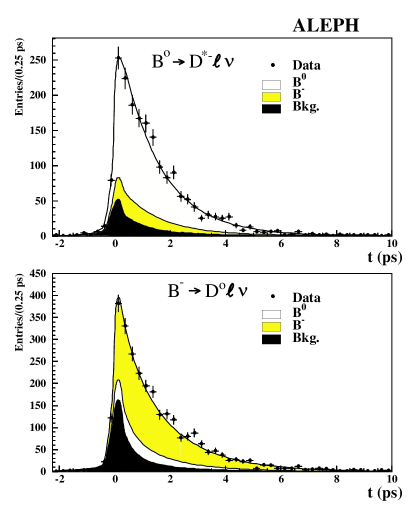
Figure 3: Proper time distributions of exclusive semi-leptonic decays from ALEPH.

A summary of the lifetimes of specific $b$-flavored hadrons is given in Figure 4 (Groom 2001). Note that the ratio of $B^{+}$ to $B^{o}$ lifetimes is 1.074$\pm$0.028, a 2.6$\sigma$ difference from unity, bordering on significance. Also, the $\Lambda_{b}$ lifetime is much shorter than the $B^{o}$ lifetime. According to proponents of the Heavy Quark Expansion model, there should be at most a 10% difference between them (Bigi 1997). To understand lifetime differences we must first analyze hadronic decays.

Figure 4: Measured lifetimes of different $B$ species.

1.3 $B$ Decay Mechanisms

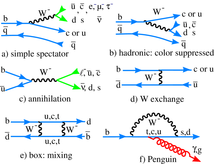
Figure 5: Various mechanisms for $B$ meson decay.

Figure 5 shows sample diagrams for $B$ decays. Semileptonic decays are depicted in Figure 5(a), when the virtual $W^{-}$ materializes as a lepton-antineutrino pair. The name “semileptonic” is given, since there are both hadrons and leptons in the final state. The leptons arise from the virtual $W^{-}$, while the hadrons come from the coupling of the spectator anti-quark with either the $c$ or $u$ quark from the $b$ quark decay. Note that the $B$ is massive enough that all three lepton species can be produced. The simple spectator diagram for hadronic decays (Figure 5(a)) occurs when the virtual $W^{-}$ materializes as a quark-antiquark pair, rather than a lepton pair. The terminology simple spectator comes from viewing the decay of the $b$ quark, while ignoring the presence of the spectator antiquark. If the colors of the quarks from the virtual $W^{-}$ are the same as the initial $b$ quark, then the color suppressed diagram, Figure 5(c), can occur. While the amount of color suppression is not well understood, a good first order guess is that these modes are suppressed in amplitude by the color factor 1/3 and thus in rate by 1/9, with respect to the non-color suppressed spectator diagram.

The annihilation diagram shown in Figure 5(c) occurs when the $b$ quark and spectator anti-quark find themselves in the same space-time region and annihilate by coupling to a virtual $W^{-}$. The probability of such a wave function overlap between the $b$ and $\bar{u}$-quarks is proportional to a numerical factor called $f_{B}$. The decay amplitude is also proportional to the coupling $V_{ub}$. The mixing and penguin diagrams will be discussed later.

Each diagram contributes differently to the decay width of the individual species. Diagram (a) is expected to be dominant. There are even more diagrams expected for baryons. Currently there is no direct evidence for diagrams (c) and (d), although (c) is expected to occur, indeed it would be responsible for the purely leptonic decay $B^{-}\to\tau^{-}\overline{\nu}$.

The semileptonic decay width, $\Gamma_{sl}$, is defined as the decay rate in units of inverse seconds into a hadron (or hadrons) plus a lepton-antineutrino pair. (Decay rates can also be expressed in units of MeV by multiplying by $h$^-.) $\Gamma_{sl}$ is related to the semileptonic branching ratio ${\cal B}_{sl}$ and the lifetime $\tau$ as

$$\Gamma_{sl}={\cal B}_{sl}\cdot\Gamma_{total}={\cal B}_{sl}/\tau~{}~{}.$$ (20)

The semileptonic width should be equal for all $b$ species. This is true for $D^{o}$ and $D^{+}$ mesons, even though their lifetimes differ by more than a factor of two. Thus, it is differences in the hadronic widths among the different $b$ species that drive the lifetime differences.

Let us now consider the case of $\overline{B}^{o}$ and $B^{-}$ lifetime differences. There is some indication that the $\overline{B}^{o}$ has a shorter lifetime, that would imply that there are more decay channels available. Figure 6 shows the color allowed and color suppressed decay diagrams for two-body decays into a ground-state charmed meson and a $\pi^{-}$. The color suppressed diagram only exists for the $B^{-}$. The relative rate

$${\Gamma(B^{-}\to D^{o}\pi^{-})\over\Gamma(\overline{B}^{o}\to D^{+}\pi^{-})}=1.8\pm 0.3~{}~{},$$ (21)

and the same is true for all other similar two-body channels, such as $D^{*}\rho^{-}$. Thus we would expect, if most $B$ decays are given by these diagrams that the $B^{-}$ would have a shorter lifetime than the $\overline{B}^{o}$, opposite of what the data suggests. An explanation is that this ratio reverses for higher multiplicity decays, but this is an interesting discrepancy that needs to be kept in mind.

Figure 6: (left) Spectator diagram for $\overline{B}^{o}\to D^{+}\pi^{-}$ and $B^{-}\to D^{o}\pi^{-}$. (right) Color suppressed spectator diagram for $B^{-}\to D^{o}\pi^{-}$ only.

2 Semileptonic $B$ Decays

2.1 Formalism of Exclusive Semileptonic $B$ Decays

The same type of semileptonic charged current decays used to find $V_{us}$ are used to find $V_{cb}$ and $V_{ub}$. The basic diagram is shown in Figure 5(a). We can use either inclusive decays, where we look only at the lepton and ignore the hadronic system at the lower vertex, or exclusive decays where we focus on a particular single hadron. Theory currently can predict either the inclusive decay rate, or the exclusive decay rate when there is only a single hadron in the final state.

Now let us briefly go through the mathematical formalism of semileptonic decays. We start with pseudoscalar $B$ to pseudoscalar $m$ transitions. The decay amplitude is given by (Grinstein 1986)(Gilman 1990)

$$A(\bar{B}\to me^{-}\bar{\nu})={G_{F}\over\sqrt{2}}V_{ij}L^{\mu}H_{\mu}{\rm,~{}where}$$ (22)

$$L^{\mu}=\bar{u}_{e}\gamma^{\mu}\left(1-\gamma_{5}\right)v_{\nu}{\rm,~{}and}$$ (23)

$$H_{\mu}=\langle m|J^{\mu}_{had}(0)|\overline{B}\rangle=f_{+}(q^{2})(P+p)_{\mu}+f_{-}(q^{2})(P-p)_{\mu},$$ (24)

where $q^{2}$ is the four-momentum transfer squared between the $B$ and the $m$, and $P(p)$ are four-vectors of the $B(m)$. $H_{\mu}$ is the most general form the hadronic matrix element can have. It is written in terms of the unknown $f$ functions that are called “form-factors.” It turns out that the term multiplying the $f_{-}(q^{2})$ form-factor is the mass of lepton squared. Thus for electrons and muons (but not $\tau$’s), the decay width is given by

$${d\Gamma_{sl}\over dq^{2}}={G_{F}^{2}|V_{ij}|^{2}K^{3}\over 24\pi^{2}}|f_{+}(q^{2})|^{2},{\rm~{}~{}where}$$ (25)

$$K={1\over 2M_{B}}\left[\left(M_{B}^{2}+m^{2}-q^{2}\right)^{2}-4m^{2}M_{B}^{2}\right]^{1/2}$$ (26)

is the momentum of the particle $m$ (with mass $m$) in the $B$ rest frame. In principle, ${d\Gamma_{sl}/dq^{2}}$ can be measured over all $q^{2}$. Thus the shape of $f_{+}(q^{2})$ can be determined experimentally. However, the normalization, $f_{+}(0)$ must be obtained from theory, for $V_{ij}$ to be measured. In other words,

$$\Gamma_{SL}\propto|V_{ij}|^{2}|f_{+}(0)|^{2}{1\over\tau_{B}}\int K^{3}g(q^{2})dq^{2},$$ (27)

where $g(q^{2})=f_{+}(q^{2})/f_{+}(0)$. Measurements of semileptonic $B$ decays give the integral term, while the lifetimes are measured separately, allowing the product $|V_{ij}|^{2}|f_{+}(0)|^{2}$ to be experimentally determined.

For pseudoscalar to vector transitions there are three independent form-factors whose shapes and normalizations must be determined (Richman 1995).

2.2 Measurement of $|V_{cb}|$

2.2.1 Heavy Quark Effective Theory and $\bar{B}\to D^{*}\ell^{-}\bar{\nu}$

We can use exclusive $B$ decays to find $V_{cb}$ coupled with “Heavy Quark Effective Theory” (HQET) (Isgur 1994). We start with a quick introduction to this theory. It is difficult to solve QCD at long distances, but it is possible at short distances. Asymptotic freedom, the fact that the strong coupling constant $\alpha_{s}$ becomes weak in processes with large $q^{2}$, allows perturbative calculations. Large distances are of the order $\sim 1/\Lambda_{QCD}\sim$1 fm, since $\Lambda_{QCD}$ is about 0.2 GeV. Short distances, on the other hand, are of the order of the quark Compton wavelength; $\lambda_{Q}\sim 1/m_{Q}$ equals 0.04 fm for the $b$ quark and 0.13 fm for the $c$ quark.

For hadrons, on the order of 1 fm, the light quarks are sensitive only to the heavy quark’s color electric field, not the flavor or spin direction. Thus, as $m_{Q}\to\infty$, hadronic systems which differ only in flavor or heavy quark spin have the same configuration of their light degrees of freedom. The following two predictions follow immediately (the actual experimental values are shown below):

$$m_{B_{s}}-m_{B_{d}} = m_{D_{s}}-m_{D^{+}}$$ (28)

$$(90.2\pm 2.5){\rm~{}MeV} (99.2\pm 0.5){\rm~{}MeV~{},~{}and}$$

$$m^{2}_{B^{*}}-m^{2}_{B} = m^{2}_{D^{*}}-m^{2}_{D}.$$ (29)

$$0.49{\rm~{}GeV^{2}} 0.55{\rm~{}GeV^{2}}.$$

The agreement is quite good but not exceptional. Since the charmed quark is not that heavy, there is some heavy quark symmetry breaking. This must be accounted for in quantitative predictions, and can probably explain the discrepancies above. The basic idea is that if you replace a $b$ quark with a $c$ quark moving at the same velocity, there should only be small and calculable changes.

In lowest order HQET there is only one form-factor function $F$ which is a function of the Lorentz invariant four-velocity transfer $\omega$, where

$$\omega={{M^{2}_{B}+M^{2}_{D^{*}}-q^{2}}\over{2M_{B}M_{D^{*}}}}.$$ (30)

The point $\omega$ equals one corresponds to the situation where the $B$ decays to a $D^{*}$ which is at rest in the $B$ frame. Here the “universal” form-factor function $F(\omega)$ has the value, $F(1)=1$, in lowest order. This is the point in phase space where the $b$ quark changes to a $c$ quark with zero velocity transfer. The idea is to measure the decay rate at this point, since we know the value of the form-factor, namely unity, and then apply the hopefully small and hopefully well understood corrections. Although this analysis can be applied to $\bar{B}\to D\ell^{-}\bar{\nu}$, overall decay rate is only 40% of $D^{*}\ell^{-}\bar{\nu}$ and the decay rate vanishes at $\omega$ equals 1 much faster, making the measurement worse.

2.2.2 Detection of $B\to D^{*}\ell\nu$

Since this is a semileptonic final state containing a missing neutrino, the decay cannot be identified or reconstructed by merely measuring the 4-vectors of the final state particles. One technique used in the past relies on evaluating the missing mass ($MM$) where

$$MM^{2} = (E_{B}-E_{D^{*}}-E_{\ell})^{2}-(\overrightarrow{p}_{\!B}-\overrightarrow{p}_{\!D^{*}}-\overrightarrow{p}_{\!\ell})^{2}$$

$$= M^{2}_{B}+M^{2}_{D^{*}}+M^{2}_{\ell}-2E_{B}\cdot(E_{D^{*}}+E_{\ell})+2E_{D^{*}}E_{\ell}$$

$$-2\overrightarrow{p}_{\!D^{*}}\cdot\overrightarrow{p}_{\!\ell}+2\overrightarrow{p}_{\!B}\cdot(\overrightarrow{p}_{\!D^{*}}+\overrightarrow{p}_{\!\ell})~{}~{}.$$

For experiments using $e^{+}e^{-}\to\Upsilon(4S)\to B\overline{B}$, the $B$ energy, $E_{B}$, is set equal to the beam energy, $E_{beam}$, and all quantities are known except the angle between the $B$ direction and the sum of the $D^{*}$ and lepton 3-vectors (the last term). A reasonable estimate of $MM^{2}$ is obtained by setting this term to zero. The signal for the $D^{*}\ell\nu$ final state should appear at the neutrino mass, namely at $MM^{2}=0$. In an alternative technique $MM^{2}$ is set to zero and the angle between the $B$ momentum and the sum of the $D^{*}$ and lepton 3-vectors is evaluated as

$$\cos\left(\Theta_{B\cdot D^{*}\ell}\right)={{2E_{B}(E_{D^{*}}+E_{\ell})-M^{2}_{B}-M^{2}_{D^{*}\ell}}\over{2\left|\overrightarrow{p}_{B}\right|\left|\left(\overrightarrow{p}_{\!D^{*}}+\overrightarrow{p}_{\!\ell}\right)\right|}}~{}~{},$$ (32)

where $M_{D^{*}\ell}$ indicates the invariant mass of the $D^{*}$-lepton combination.

A Monte-Carlo simulation of $\cos\left(\Theta_{B\cdot D^{*}\ell}\right)$ is given for the final state of interest and for the main background reaction in Figure 7. For the correct final state only a few events are outside the “legal” region of $\pm 1$, while when there are extra pions in the final state the shape changes and many events are below $-1$.

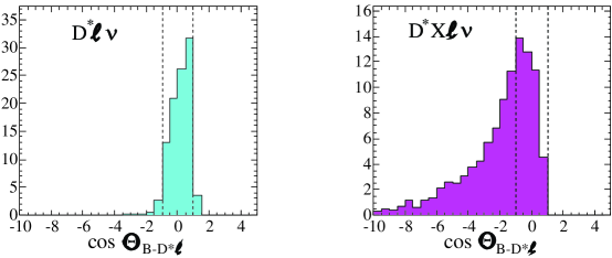
Figure 7: The cosine of the angle between the $B$ momentum vector and the sum of $D^{*}$ and lepton momentum vectors for (left) the final state $D^{*}\ell\nu$ and (right) $D^{*}X\ell\nu$, where $X$ refers to an additional pion.

Recent CLEO data has been analyzed with such a technique. The data in two specific $\omega$ bins is shown in Figure 8. The final result for all $\omega$ bins is shown in Figure 9. The result is characterized by both a value for $F(1)|V_{cb}|$ and a shape parameter $\rho^{2}$.

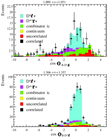
Figure 8: The signal and background contributions in two different $\omega$ bins for the final state $D^{*}\ell\nu$.

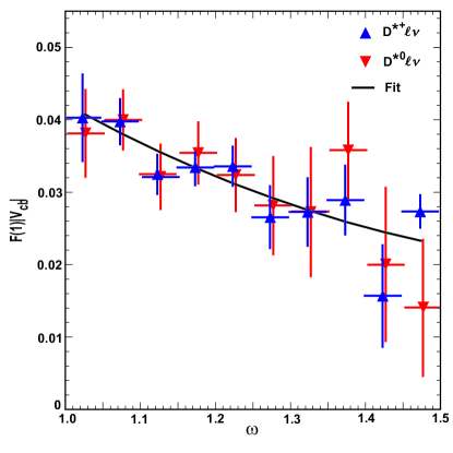
Figure 9: The CLEO results for $D^{*}\ell\nu$ for both $\overline{B}^{o}$ and $B^{-}$. The curve is a fit to a shape suggested in (Caprini 1998).

2.2.3 Evaluation of $V_{cb}$ Using $B\to D^{*}\ell\nu$

Figure 10 and Table 1 give recent experimental results on exclusive $B\to D^{*}\ell\nu$ decays. The CLEO results are not in particularly good agreement with the rest of the world including the BELLE results.

Table 1: Modern Determinations of $F(1)|V_{cb}|$ using $B\to D^{*}\ell^{-}\overline{\nu}$ decays

Experiment	$F(1)|V_{cb}|$ $(\times 10^{-3})$	$\rho^{2}$
ALEPH (Buskulic 1997)	$33.0\pm 2.1\pm 1.6$	$0.74\pm 0.3\pm 0.4$
BELLE (Tajima 2001)	$35.4\pm 1.9\pm 1.9$	$1.35\pm 0.17\pm 0.18$
CLEO (Heltsley 2001)	$42.2\pm 1.3\pm 1.8$	$1.61\pm 0.09\pm 0.21$
DELPHI (Abreu 2001)	$34.5\pm 1.4\pm 2.5$	$1.2\pm 0.1\pm 0.4$
OPAL($\pi\ell$) (Abbiendi 2000)	$37.9\pm 1.3\pm 2.4$	$1.2\pm 0.2\pm 0.4$
OPAL (Abbiendi 2000)	$37.5\pm 1.7\pm 1.8$	$1.4\pm 0.2\pm 0.2$
Average	$37.8\pm 1.4$	1.37$\pm$ 0.13

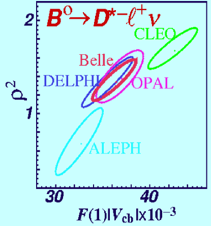
Figure 10: The correlation between the slope parameter $\rho^{2}$ and $F(1)|V_{cb}|$. The contours are for a change in the fit $\chi^{2}$ of one unit.

To extract the value of $|V_{cb}|$ we have to determine the corrections to $F(1)$ that lower its value from unity. The corrections are of two types: quark mass, characterized as some coefficient times $\Lambda_{QCD}/m_{Q}$, and hard gluon, characterized as $\eta_{A}$. The value of the form-factor can then be expressed as (Neubert 1996)

$$F(1)=\eta_{A}\left(1+0\cdot\Lambda_{QCD}/m_{Q}+c_{2}\cdot\left(\Lambda_{QCD}/m_{Q}\right)^{2}+....\right)=\eta_{A}(1+\delta).$$ (33)

The zero coefficient in front of the $1/m_{Q}$ term reflects the fact that the first order correction in quark mass vanishes at $\omega$ equals one. This is called Luke’s Theorem (Luke 1990). Recent estimates are 0.967$\pm$0.007 and $-0.55\pm$0.025 for $\eta_{A}$ and $\delta$, respectively. The value predicted for $F(1)$ then is 0.91$\pm$0.05. This is the conclusion of the PDG review done by Artuso and Barberio (Artuso 2001). There has been much controversy surrounding the theoretical prediction of this number. In the future Lattice-Gauge Theory calculations will presumably become accurate when unquenched. (Quenched calculations are those performed without light quark loops.) Current lattice calculations give $F(1)=0.913^{+0.024}_{-0.017}\pm 0.016^{+0.003+0.000+0.006}_{-0.014-0.016-0.014}$, where the uncertainties come respectively, from statistics and fitting, matching lattice gauge theory to QCD, lattice spacing dependence, light quark mass effects and the quenching approximation. (Hashimoto 2001).

Using the Artuso-Barberio value for $F(1)$ we have

$$\left|V_{cb}\right|=(41.5\pm 1.5\pm 2.3)\times 10^{-3}~{}~{},$$ (34)

where the first error is experimental and the second the error on the calculation of $F(1)$.

2.2.4 $|V_{cb}|$ from Inclusive Semileptonic Decays

The inclusive semileptonic branching ratio $b\to X\ell\nu$ has been measured by both CLEO and LEP to reasonable accuracy. CLEO finds $(10.49\pm 0.17\pm 0.43)$%, while LEP has $(10.56\pm 0.11\pm 0.18)$%. These are not quite the same quantities as the CLEO number is an average over $B^{-}$ and $B^{o}$ only, while the LEP number is a weighted average over all $b$ hadron species produced in $Z^{o}$ decays. Thus using the LEP number one should use the average “$b$ quark” lifetime of 1.560$\pm$0.014 ps.

Using the Heavy Quark Expansion, HQE, model (Bigi 1997) we can relate the total semileptonic decay rate at the quark level to $|V_{cb}|$ as

$$\left|V_{cb}\right|^{2} = h(\lambda_{1},\lambda_{2},\overline{\Lambda})\times\Gamma(b\to c\ell\nu)$$

$$= h(\lambda_{1},\lambda_{2},\overline{\Lambda})\times{\cal{B}}(b\to c\ell\nu)/\tau_{b}~{}~{},$$

where ${\cal{B}}(b\to c\ell\nu)$ is the inclusive semileptonic branching ratio minus a small $b\to u\ell\nu$ component. (It is precisely the decay of a $B$ meson to a lepton-antineutrino pair plus any charmed hadron.) $\tau_{b}$ is the lifetime of that particular meson or average lifetime of the combination of the $b$-flavored hadrons used in the analysis, suitably weighted. In HQE the semileptonic rate is described to order $\left(\Lambda_{QCD}/m_{b}\right)^{2}$ by the parameters:

• $\lambda_{1}={M_{B}\over 2}\langle B(v)\left|\overline{h_{v}}(iD)^{2}h_{v}\right|B(v)\rangle$, is the kinetic energy of the residual motion of the $b$ quark in the hadron

• $\lambda_{2}=-{M_{B}\over 2}\langle B(v)\left|\overline{h_{v}}{g\over 2}\cdot\sigma^{\mu\nu}G_{\mu\nu}h_{v}\right|B(v)\rangle$, is the chromo-magnetic coupling of the $b$ quark spin to the gluon field.

• $\overline{\Lambda}=\overline{M_{B}}-m_{b}+{\lambda_{1}\over 2M_{B}}$, is the strong interaction coupling where $\overline{M_{B}}$ is the spin averaged $B$ meson mass, $(M_{B}+3M_{B^{*}})/4$.

These parameters are further related as

$$M_{B}=m_{b}+\overline{\Lambda}-{{(\lambda_{1}+3\lambda_{2})}\over{2m_{b}}}$$ (36)

$$M_{B^{*}}=m_{b}+\overline{\Lambda}-{{(\lambda_{1}-\lambda_{2})}\over{2m_{b}}}~{}~{}.$$

These relations allow us to determine $\lambda_{2}$ from the $M_{B^{*}}-M_{B}$ mass splitting as 0.12 GeV². The function $h(\lambda_{1},\lambda_{2},\overline{\Lambda})$ can be calculated from the Heavy Quark Expansion (HQE) model. This involves both perturbative and non-perturbative pieces.

Although we will go through this example there is a disturbing aspect of assuming quark-hadron duality; the idea of duality is that if you integrate over enough exclusive charm bound states and enough phase space, the inclusive hadronic result will match the quark level calculation. However, we do not know what size is the uncertainty associated with the duality assumption. In fact, Isgur said “I identify a source of $\Lambda_{QCD}/m_{Q}$ corrections to the assumption of quark-hadron duality in the application of heavy quark methods to inclusive heavy quark decays. These corrections could substantially affect the accuracy of such methods in practical applications and in particular compromise their utility for the extraction of the CKM matrix element $V_{cb}$” (Isgur 1999).

Let us move to the details of the calculation. In one implementation $\lambda_{1}$ and $\overline{\Lambda}$ are derived; the relationship between the inclusive $b\to c\ell\nu$ branching fraction (about 99% of $b\to X\ell\nu$) is given as

$$\left|V_{cb}\right|= 0.0411\sqrt{{{\cal{B}}(b\to X_{c}\ell\nu)}\over{0.105}}\sqrt{1.55~{}{\rm ps}\over\tau_{b}}\left(1-0.012{{\mu_{\pi}^{2}-0.5~{}{\rm GeV}^{2}}\over{0.1~{}\rm{GeV}^{2}}}\right)$$

$$\times\left(1\pm 0.015_{pert.}\pm 0.010_{m_{b}}\pm 0.012_{1/m_{Q}^{3}}\right)~{}~{},$$

where $\mu_{\pi}^{2}$ is the negative of $\lambda_{1}$ modulo QCD corrections and is taken as $(0.5\pm 0.1)$ GeV² (Bigi 1997).

This leads to a value of

$$\left|V_{cb}\right|=(40.7\pm 0.5\pm 2.4)\times 10^{-3}$$ (39)

from the LEP data alone, with a similar value from CLEO. The first error contains the statistical and systematic error from the experiments while the second error contains an estimate of the theory error from sources other than duality.

In another implementation the parameters $\lambda_{1}$ and $\overline{\Lambda}$ are obtained from data. Here we use the HQE formula

$$\Gamma_{sl}={{G_{F}^{2}\left|V_{cb}\right|^{2}M_{B}^{5}}\over{192\pi^{3}}}0.369\times$$

$$\left[1-1.54{\alpha_{s}\over\pi}-1.65{{\overline{\Lambda}}\over M_{B}}\left(1-1.087{\alpha_{s}\over\pi}\right)-0.95{\overline{\Lambda}^{2}\over M_{B}^{2}}-3.18{\lambda_{1}\over M_{B}^{2}}+0.02{\lambda_{2}\over M_{B}^{2}}\right]~{}.$$

Determining $\lambda_{1}$ and $\overline{\Lambda}$ can be accomplished by measuring, for example, the “moments” of the hadronic mass produced in $b\to c\ell\nu$ decays. The first moment is defined as the deviation from the $D$ mass ($M_{D}$) as $\langle M_{X}^{2}-\overline{M}_{D}^{2}\rangle$ and the second moment as $\langle\left(M_{X}^{2}-\overline{M}_{D}^{2}\right)^{2}\rangle$. It is also possible to use the first and second moments of the lepton energy distribution in these decays, or moments of the photon energy in the process $b\to s\gamma$. In fact any two distributions can be used; in practice it will be critical to use all of them to try and ascertain if any violations of quark-hadron duality appear and to check that terms of order $\left(\Lambda_{QCD}/m_{b}\right)^{3}$ are not important.

CLEO has used the first and second moments of the hadron mass in $b\to c\ell\nu$ decays. They find the $M_{X}$ distributions by using missing energy and momentum in the event to define the $\nu$ four-vector. Then detecting only the lepton and requiring it to have a momentum above 1.5 GeV/c, they calculate:

$$M_{X}^{2} = \left(E_{B}-E_{\ell}-E_{\nu}\right)^{2}-\left(\overrightarrow{p}_{\!B}-\overrightarrow{p}_{\!\ell}-\overrightarrow{p}_{\!\nu}\right)^{2}$$ (41)

$$= M_{B}^{2}+M^{2}_{\ell\nu}-2E_{B}\left(E_{\ell}+E_{\nu}\right)+2\overrightarrow{p}_{\!B}\cdot\left(\overrightarrow{p}_{\!\ell}-\overrightarrow{p}_{\!\nu}\right)$$

$$\approx M_{B}^{2}+M^{2}_{\ell\nu}-2E_{B}E_{\ell\nu}~{}~{},$$

where $M_{\ell\nu}$ is the invariant mass of the lepton-neutrino pair. The measured $M_{X}^{2}$ distribution is shown in Figure 11. We do not see distinct peaks at the mass of the $D$ and $D^{*}$ mesons because ignoring the last term in equation (41) causes poor resolution. This term must be ignored, however, using this technique because we do not know the direction of the $B$ meson.

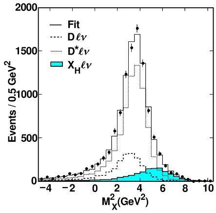
Figure 11: The mass distribution for $b\to c\ell\nu$ events from CLEO. X_H indicates an additional pion plus a $D$ or $D^{*}$.

CLEO finds values of the first and second moments of (0.287$\pm$0.023$\pm$0.061) GeV² and (0.712$\pm$0.056$\pm$0.176) GeV⁴, respectively. These lead to the determination of $\lambda_{1}$, $\overline{\Lambda}$ and $V_{cb}$ shown in Figure 12. Later we will see a different determination using $b\to s\gamma$ (section 5.3.1).

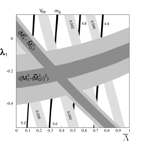
Figure 12: Constraints in $\lambda_{1}$ versus $\overline{\Lambda}$ from CLEO measurements of first and second hadronic moments in semileptonic decay. The darker band gives experimental uncertainties alone, while the lighter outer band also includes uncertainties from unknown 3rd order theoretical parameters. Bands of constant $V_{cb}$ and $b$ quark mass, $m_{b}$, are also shown, where the band widths represents theoretical uncertainties due to unknown 3rd order parameters.

In summary the exclusive measurements of $V_{cb}$ are to be trusted while the inclusive determination, though consistent, has an unknown source of systematic error and should not be used now.

2.3 Measurement of $|V_{ub}|$

This is a heavy to light quark transition where HQET cannot be used directly as in finding $V_{cb}$. Unfortunately the theoretical models that can be used to extract a value from the data do not currently give precise predictions.

Three techniques have been used. The first measurement of $V_{ub}$ done by CLEO (Fulton 1990) and subsequently confirmed by ARGUS (Albrecht 1990), used only leptons which were more energetic than those that could come from $b\to c\ell^{-}\bar{\nu}$ decays. These “endpoint leptons” can occur $b\to c$ background free at the $\Upsilon(4S)$, because the $B$’s are almost at rest. The CLEO data are shown in Figure 13. Since the lepton momentum for $B\to D\ell\nu$ decays is cut off by phase space, this data provides incontrovertible evidence for $b\to u\ell\nu$ decays.

Figure 13: Sum of inclusive electron and muon distributions from CLEO. The solid points are data taken on the peak of the $\Upsilon(4S)$ while the open circles are data taken on the continuum 30 MeV below the resonance(suitably normalized). The dashed line is a fit to the continuum data and the solid line is the predicted curve from $b\to c\ell\nu$ dominated by $B\to D\ell\nu$ near the end of the allowed lepton spectrum.

Unfortunately, there is only a small fraction of the $b\to u\ell^{-}\bar{\nu}$ lepton spectrum that can be seen this way, leading to model dependent errors. The models used are either inclusive predictions, sums of exclusive channels, or both (Isgur 1995) (Bauer 1989) (Körner 1989) (Melikhov 1996) (Altarelli 1982) (Ramirez 1990). The average among the models is $|V_{ub}/V_{cb}|=0.079\pm 0.006$, without a model dependent error. These models differ by at most 11%, making it tempting to assign a $\pm$6% error. However, there is no quantitative way of estimating the error.

ALEPH (Barate 1999), L3 (Acciarri 1998) and DELPHI (Abreu 2000) isolate a class of events where the hadron system associated with the lepton is enriched in $b\to u$ and thus depleted in $b\to c$. They define a likelihood that hadron tracks come from $b$ decay by using a large number of variables including, vertex information, transverse momentum, not being a kaon etc.. Then they require the hadronic mass to be less than 1.6 GeV, which greatly reduces $b\to c$, since a completely reconstructed $b\to c$ decay has a mass greater than that of the $D$ (1.83 GeV). They then examine the lepton energy distribution, shown in Figure 14 for DELPHI.

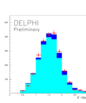
Figure 14: The lepton energy distribution in the $B$ rest frame from DELPHI. The data have been enriched in $b\to u$ events, and the mass of the recoiling hadronic system is required to be below 1.6 GeV. The points indicate data, the light shaded region, the fitted background and the dark shaded region, the fitted $b\to u\ell\nu$ signal.

The average of all three results is $|V_{ub}|=(4.13^{+0.42+0.43+0.24}_{-0.47-0.48-0.25}\pm 0.20)\times 10^{-3}$, resulting in a value for $|V_{ub}/V_{cb}|=0.102\pm 0.018$, using $|V_{cb}|=0.0405\pm 0.0025$. I have several misgivings about this result. First of all the experiments have to understand the systematic errors very well. To understand semileptonic $b$ and $c$ decays and thus find their $b\to u\ell\nu$ efficiency, they employ different models and Monte Carlo manifestations of these models. To find the error they take half the spread that different models give. This alone may be a serious underestimate. Secondly they use one model, the HQE model, to translate their measured rate to a value for $|V_{ub}|$. This model assumes duality, and there are no successful experimental checks: The model fails on the $\Lambda_{b}$ lifetime prediction. Furthermore, the quoted theoretical error, even in the context of the model, has been estimated by Neubert to be much larger at 10% (Neubert 2000). Others have questioned the effect of the hadron mass cut and estimate 10-20% errors due to this alone (Bauer 2001).

It may be possible to use the spectrum of photons in $b\to s\gamma$ to reduce the theoretical error in the endpoint lepton method or to make judicious cuts in $q^{2}$ instead of hadronic mass to help reduce the theoretical errors. See (Wise 2001) for an erudite discussion of these points.

The third method uses exclusive decays. CLEO has measured the decay rates for the exclusive final states $\pi\ell\nu$ and $\rho\ell\nu$ (Alexander 1996). The data are shown in Figure 15. The model of Körner and Schuler (KS) is ruled out by the measured ratio of $\rho/\pi$. Other models include those of (Isgur 1995) (Isgur 1989) (Wirbel 1985) (Bauer 1989) (Korner 1988) (Melikhov 1996) (Altarelli 1982) (Ramierz 1990). CLEO has presented an updated analysis for $\rho\ell\nu$ where they have used several different models to evaluate their efficiencies and extract $V_{ub}$. These theoretical approaches include quark models, light cone sum rules (LCRS), and lattice QCD. The CLEO values are shown in Table 2.

Figure 15: The $B$ candidate mass distributions and the signal bin lepton momentum spectra (insets) for the pion modes (top) and the sum of $\rho$ and $\omega$ (vector) modes (bottom). The points are the data after continuum and fake background subtractions; the dark-shaded, cross-hatched and unshaded histograms are $b\to cX$, $b\to u\ell\nu$ feed-down and signal, respectively. For the $\pi$ (vector) modes, the light-shaded and hatched histograms are $\pi$ $\to$ $\pi$ (vector$\to$ vector) and vector $\to$ $\pi$ ($\pi$ $\to$ vector) cross-feed, respectively (charge final states can feed neutral and vice-versa). The histogram normalizations are from the nominal fit. The arrows indicate the momentum cuts.

Table 2: Values of $|V_{ub}|$ using $B\to\rho\ell^{-}\overline{\nu}$ and some theoretical models

Model	$V_{ub}$ $(\times 10^{-3})$
ISGW2 (Isgur 1989)	$3.23\pm 0.14^{+0.22}_{-0.29}$
Beyer/Melikhov (Beyer 1998)	$3.32\pm 0.15^{+0.21}_{-0.30}$
Ligeti/Wise (Ligeti 1996)	$2.92\pm 0.13^{+0.19}_{-0.26}$
LCSR (Ball 1998)	$3.45\pm 0.15^{+0.22}_{-0.31}$
UKQCD (Debbio 1998)	$3.32\pm 0.14^{+0.21}_{-0.30}$

The uncertainties in the quark model calculations (first three in the table) are guessed to be 25-50% in the rate. The Ligeti/Wise model uses charm data and SU(3) symmetry to reduce the model dependent errors. The other models estimate their errors at about 30-50% in the rate, leading conservatively to a 25% error in $|V_{ub}|$. Note that the models differ by 18%, but it would be incorrect to assume that this spread allows us to take a smaller error. It may be that the models share common assumptions, e.g. the shape of the form-factors. At this time it is prudent to assign a 25% model dependent error realizing that the errors in the models cannot be averaged. The fact that the models do not differ much allows us to comfortably assign a central value $|V_{ub}|=(3.25\pm 0.14^{+0.22}_{-0.29}\pm 0.80)\times 10^{-3}$, and a derived value $|V_{ub}/V_{cb}|=0.08\pm 0.02$ .

Lattice QCD has predicted form-factors and resulting rates for the exclusive semileptonic final states $\pi\ell\nu$ and $\rho\ell\nu$ (Sachrajda 1999) in the quenched approximation. These calculations require the momentum of the final-state light meson to be small in order to avoid discretization errors. This means we only obtain results at large values of the invariant four-momentum transfer squared, $q^{2}$. Figure 16 shows the predictions of the $B\to\rho\ell\nu$ width as a function of $q^{2}$. Note that the horizontal scale is highly zero suppressed. The region marked “phase space only” is not calculated but estimated using a phase space extrapolation from the last lattice point.

Figure 16: The UKQCD lattice calculation for $B\to\rho\ell\nu$ shown as circles. The line is an estimate.

The integral over the region for $q^{2}$ $>$ 14 GeV² gives a rate of $\Delta\Gamma=8.3\left|V_{ub}\right|^{2}$ ps^-1-GeV². The CLEO measurement in the same interval gives $(7.1\pm 2.4)\times 10^{-5}$ps^-1-GeV², which yields a value for $V_{ub}=(2.9\pm 0.5)\times 10^{-3}$ (Sachrajda 1999). Ultimately unquenched lattice calculations when coupled with more precise data will yield a much better value for $V_{ub}$.

3 Facilities for $b$ Studies

3.1 $b$ Production Mechanisms

Although most of what is known about $b$ physics presently has been obtained from $e^{+}e^{-}$ colliders operating either at the $\Upsilon(4S)$ or at LEP, interesting information is now appearing from the hadron collider experiments, CDF and D0, which were designed to look for considerably higher energy phenomena. The appeal of hadron colliders arises mainly from the large measured $b$ cross-sections. At the FNAL collider, 1.8 TeV in the $p\bar{p}$ center-of-mass, the cross-section has been measured as $\sim$100 $\mu$b, while it is expected to be about five times higher at the LHC (Artuso 1994).

The different production mechanisms of $b$ quarks at various accelerators leads to dissimilar methods of measurements. Figure 17 shows the production of $B^{-}$ and $B^{o}$ mesons at the $\Upsilon(4S)$, while Figure 18 shows the production mechanism of the different $b$ species at a higher energy $e^{+}e^{-}$ collider such as LEP. Figure 19 shows the production mechanisms for a heavy $b$ or $c$ quark.

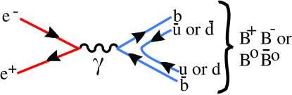
Figure 17: $B$ production at the $\Upsilon(4S)$.

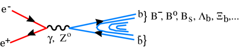
Figure 18: $b$ production in the continuum at $e^{+}e^{-}$ colliders.

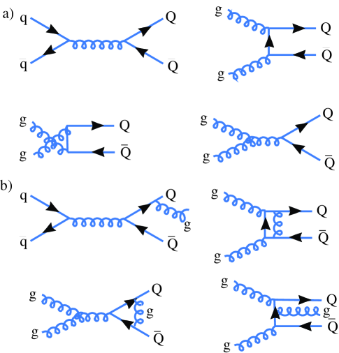
Figure 19: Heavy quark, $Q$, production at hadron colliders. (a) Second order in $\alpha_{s}$, while (b) is third order.

At the $\Upsilon(4S)$ the total $b$ production cross-section is 1.05 nb. In hadron colliders the measured cross-section is about 100$\mu$b. The third order diagrams appear about as important as the second order diagrams and the overall theoretical calculation gives about 1/2 of the measured value.

3.2 Accelerators for $b$ Physics

Experiments on $b$ decays started with CLEO and ARGUS using $e^{+}e^{-}$ colliders operating at the $\Upsilon(4S)$ and were quickly joined by the PEP and PETRA machines operating around 30 GeV. Table 3 lists some of the machines used to study $b$ quarks in the last century (Artuso 1994).

Table 3: Machines used for $b$ physics in the 20th century. The total number of $\overline{b}b$ pairs accumulated per experiment is also listed when known.

Machine	Beams	Energy	$\sigma(b)$	$b$ fraction	${\cal{L}}$	Total #
		(GeV)			cm-2s-1	$b$-pairs
CESR	$e^{+}e^{-}$	10.8	1.05 nb	0.25	1.3$\times 10^{33}$	$9.8\times 10^{6}$
DORIS	$e^{+}e^{-}$	10.8	1.05 nb	0.23	$\sim 10^{31}$	$0.4\times 10^{6}$
PEP	$e^{+}e^{-}$	29	0.4 nb	0.09	3.2$\times 10^{31}$
PETRA	$e^{+}e^{-}$	35	0.3 nb	0.09	1.7$\times 10^{31}$
LEP	$e^{+}e^{-}$	91	9.2 nb	0.22	2.4$\times 10^{31}$	$1.8\times 10^{6}$
SLC	$e^{+}e^{-}$	91	9.2 nb	0.22	3.0$\times 10^{30}$	$8.8\times 10^{4}$
TEVATRON	$\overline{p}p$	1800	100 $\mu$b	0.002	3$\times 10^{31}$

In the year 2000 the PEP II and KEK-B storage ring accelerators began operation. These machines have separate $e^{-}$ and $e^{+}$ magnet rings so they can operate at asymmetric energies; PEP II has beam energies of 9.0 GeV and 3.1 GeV, while KEK-B has energies of 8.0 GeV and 3.5 GeV. This allows the $B$ meson to move with velocity $\beta\sim 0.6$, which turns out to be very important in measurements of CP violation, since time integrated CP violation via mixing must be exactly zero due to the C odd nature of the $\Upsilon(4S)$. These machines also make very high luminosities. Current and future machines for $B$ physics are listed in Table 4. The CDF and D0 experiments will continue at the Tevatron with higher luminosities. CDF has already made significant contributions including studies of $b$ production, lifetimes and the discovery of the $B_{c}$ meson (Abe 1998). BTeV and LHCb will go into operation around 2007 with much larger event rates. The CMS and ATLAS experiments at the LHC will also contribute to $b$ physics especially in the early stages when the luminosity will be relatively low; at design luminosity these experiments have an average of 23 interactions per crossing making finding of detached vertices difficult.

Table 4: Machines in use or approved for dedicated $b$ physics experiments.

Machine	Exp.	Beam	Energy	$\sigma(b)$	$b$	${\cal{L}}$(Design)	Interactions
			(GeV)		fraction	cm-2s-1	per crossing
PEP II	BABAR	$e^{+}e^{-}$	10.8	1.05 nb	1/4	3$\times 10^{33}(\dagger)$	$\ll 1$
KEK-B	BELLE	$e^{+}e^{-}$	10.8	1.05 nb	1/4	$10^{34}$	$\ll 1$
HERA	HERA-b	$pN$	800	10 nb	$2\cdot 10^{-6}$		4
Tevatron	BTeV	$\overline{p}p$	2000	100 $\mu$b	1/500	2$\times 10^{32}$	2
LHC	LHCb	$\overline{p}p$	14000	500 $\mu$b	1/160	2$\times 10^{32}$	0.6
$\dagger$ Machine has already exceeded design luminosity.

3.3 $e^{+}e^{-}$ Detectors

Most experiments at $e^{+}e^{-}$ storage rings look quite similar. CLEO II, shown in Figure 20, was the first detector to have both an excellent tracking system and an excellent electromagnetic calorimeter.

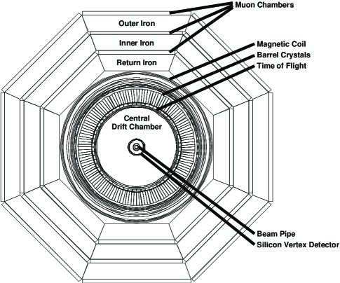
Figure 20: Electrons view of the CLEO II detector.

Starting from the inside there is a thin beryllium beam pipe surrounded by a silicon vertex detector; this detector measures positions very accurately on the order of 10 $\mu$m. Then there is a wire drift chamber whose main function is to measure the curving trajectories of particles in the 1.5T solenoidal magnetic field. The next device radially outward is time-of-flight system to distinguish pions, kaons and protons. This system only works for lower momenta. The most important advance in the CLEO III, BELLE and BABAR detectors is much better charged hadron identification. Each experiment uses different techniques based on Cherenkov radiation to extend $\pi/K$ separation up to the limit from $B$ decays. The next device is an electromagnetic calorimeter that uses Thallium doped CsI crystals; indeed this was the most important new technical implementation done in CLEO II and has also been adopted by BABAR and BELLE. Afterwards there is segmented iron that serves as both a magnetic flux return and a filter for muon identification.

Figure 21 shows a view of the BELLE detector parallel to the beam.

Figure 21: through the BELLE detector.

3.4 $b$ Production Characteristics at Hadron Colliders

To make precision measurements, large samples of $b$’s are necessary. Fortunately, these are available. With the Fermilab Main Injector, the Tevatron collider will produce $\approx 4\times 10^{11}$ $b$ hadrons/$10^{7}$ s at a luminosity of $2\times 10^{32}$cm^-2s^-1. These rates compare very favorably to e⁺e^- machines operating at the $\Upsilon$(4S). At a luminosity of $10^{34}$cm^-2s^-1 they would produce $2\times 10^{8}$ B’s/$10^{7}$ s. Furthermore $B_{s}$, $\Lambda_{b}$ and other $b$-flavored hadrons are accessible for study at hadron colliders. The LHC has about a five times larger $b$ production cross-section. Also important are the large charm rates, $\sim$10 times larger than the $b$ rate.

In order to understand the detector design it is useful to examine the characteristics of $b$ quark production at $p\overline{p}$ collider. It is often customary to characterize heavy quark production in hadron collisions with the two variables $p_{t}$ and $\eta$, where $\eta=-ln\left(\tan\left({\theta/2}\right)\right),$ and $\theta$ is the angle of the particle with respect to the beam direction. According to QCD based calculations of $b$ quark production, the $B$’s are produced “uniformly” in $\eta$ and have a truncated transverse momentum, $p_{t}$, spectrum characterized by a mean value approximately equal to the $B$ mass (Artuso 1994). The distribution in $\eta$ is shown in Figure 22(a). Note that at larger values of $|\eta|$, the $B$ boost, $\beta\gamma$, increases rapidly (b).

The “flat” $\eta$ distribution hides an important correlation of $b\bar{b}$ production at hadronic colliders. In Figure 22(c) the production angles of the hadron containing the $b$ quark is plotted versus the production angle of the hadron containing the $\bar{b}$ quark according to the Pythia generator. Many important measurements require the reconstruction of a $b$ decay and the determination of the flavor of the other $\bar{b}$, thus requiring both $b$’s to be observed in the detector. There is a very strong correlation in the forward (and backward) direction: when the $B$ is forward the $\overline{B}$ is also forward. This correlation is not present in the central region (near 90^∘). By instrumenting a relative small region of angular phase space, a large number of $b\bar{b}$ pairs can be detected. Furthermore the $B$’s populating the forward and backward regions have large values of $\beta\gamma$.

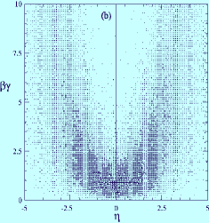
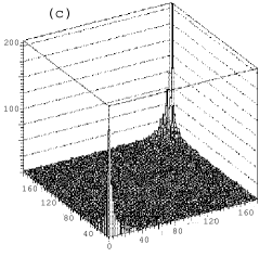
Figure 22: (a) The $B$ yield versus $\eta$. (b) $\beta\gamma$ of the $B$ versus $\eta$. (c) The production angle (in degrees) for the hadron containing a $b$ quark plotted versus the production angle for a hadron containing $\bar{b}$ quark.

BTeV, a dedicated heavy flavor experiment approved to run at the Fermilab Tevatron collider, uses two forward spectrometers (along both the $p$ and $\overline{p}$ directions) that utilize the boost of the $B$’s at large rapidities. This is of crucial importance because the main way to distinguish $b$ decays is by the separation of decay vertices from the main interaction. LHCb, approved for operation at the LHC, needs a larger detector to analyze the higher momentum decay products, and thus has only one arm.

3.4.1 The BTeV Detector Description

I will describe BTeV here though LHCb shares many of the same considerations. There are difficulties that heavy quark experiments at hadron colliders must overcome. First of all, the huge $b$ rate is accompanied by an even larger rate of uninteresting interactions. At the Tevatron the $b$-fraction is only 1/500. In searching for rare processes, at the level of parts per million, the background from $b$ events is dominant. (Of course all $b$ experiments have this problem.) The large data rate of $b$’s must be handled. For example, BTeV, has 1 kHz of $b$’s into the detector, and these events must be selected and written out. The electromagnetic calorimeter must be robust enough to deal with the particles from the underlying event and still have useful efficiency. Furthermore, radiation damage can destroy detector elements.

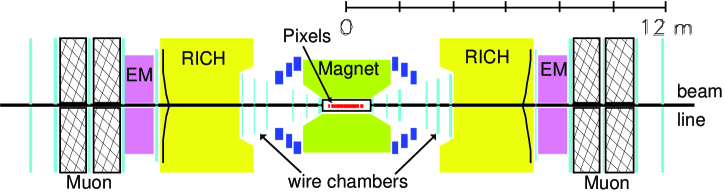
Figure 23: Schematic of the BTeV detector.

The BTeV Detector is shown in Figure 23 (Skwarnicki 2001) and the LHCb detector in Figure 24 (Muheim 2001). The central part of the BTeV detector has a silicon pixel detector inside a 1.5 T dipole magnet. The LHCb experiment uses silicon strips. The BTeV pixel detector provides precision space points for use in both the offline analysis and the trigger. The pixel geometry is sketched in Figure 25(a). Pulse heights are measured on each pixel. Prototype detectors were tested in a beam at Fermilab; excellent resolutions were obtained, especially when reading out pulse heights (Appel 2001) (see Figure 25(b)). The final design uses a 3-bit ADC.

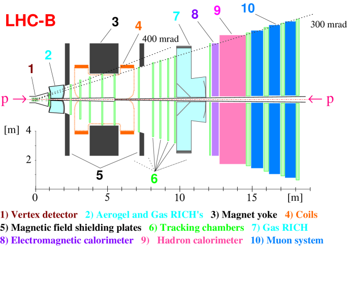
Figure 24: A schematic diagram of the LHCb detector.

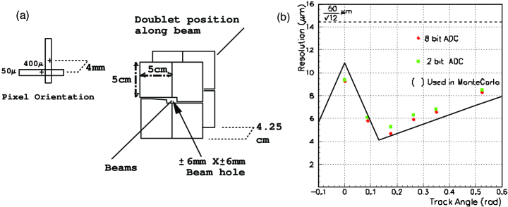
Figure 25: (a) Pixel detector geometry in BTeV. The detector is inside the beam pipe. (b) The spatial resolution as a function of the incident track angle for both 2-bit and 8-bit ADC’s as measured in an 800 GeV/c pion beam. The straight lines are piecewise fits to the data used in the Monte Carlo simulation. The dashed line near the top indicates the resolution obtainable without using pulse height information.

The pixel tracker provides excellent vertex resolution, good enough to trigger on events with detached vertices characteristic of $b$ or $c$ decays. BTeV shows a rejection of 100:1 for minimum bias events in the first trigger level while accepting about 50% of the usable $b$ decays. A good explanation of the trigger algorithm can be found at
http://www-btev.fnal.gov/public_documents/animations/Animated_Trigger/  . Further trigger levels reduce the background by about a factor of twenty while decreasing the $b$ sample by only 10%. The trigger system stores data in a pipeline that is long enough to ensure no deadtime. The data acquisition system has sufficient throughput to accommodate an output of 1 kHz of $b$’s, 1 kHz of $c$’s and 2 kHz of junk. Tracking is accomplished using straw tube wire chambers with silicon strip chambers in the high track density region near the beam.

Charged particle identification is done using a Ring Imaging CHerenkov detector. A gaseous C₄F₁₀ radiator is used with a large mirror that focuses light on plane of photon detectors; these currently are Hybrid Photo-Diodes. They have a photocathode and a 20 KV potential difference between the photocathode and a silicon diode that is segmented into 163 individual pads. The photoelectron is accelerated and focused onto the diode yielding position information for the initial photon. The system will provide four standard-deviation kaon/pion separation between 3-70 GeV/c, electron/pion separation up to 22 GeV/c and pion/muon separation up to 15 GeV/c. Because protons don’t radiate until 9 GeV/c they can’t be distinguished from kaons below this momenta. BTeV is considering an additional liquid C₆F₁₄ radiator, 1 cm thick, in the front of the gas along with a proximity focused phototube array adjacent to the sides of the gas volume, to resolve this ambiguity.

In addition, BTeV has an excellent Electromagnetic calorimeter made from PbWO₄ crystals, based on the design of CMS. Finally, the Muon system is used to both identify muons and provide an independent trigger on dimuons (BTeV 2000).

4 $B^{o}-\overline{B}^{o}$ Mixing

4.1 Introduction

Neutral $B$ mesons can transform to their anti-particles before they decay. The diagrams for this process are shown in Figure 26 for the $B_{d}$. There is a similar diagram for the $B_{s}$. Although $u$, $c$ and $t$ quark exchanges are all shown, the $t$ quark plays a dominant role mainly due to its mass, as the amplitude of this process is proportional to the mass of the exchanged fermion.

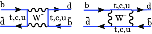
Figure 26: The two diagrams for $B_{d}$ mixing.

Under the weak interactions the eigenstates of flavor, degenerate in pure QCD can mix. Let the quantum mechanical basis vectors be $\{|1\rangle,|2\rangle\}\equiv\{|B^{o}\rangle,|\overline{B}^{o}\rangle\}$. Then the Hamiltonian is

$${\cal H}=M-{i\over 2}\Gamma=\left(\begin{array}[]{cc}M&M_{12}\\ M_{12}^{*}&M\end{array}\right)-{i\over 2}\left(\begin{array}[]{cc}\Gamma&\Gamma_{12}\\ \Gamma_{12}^{*}&\Gamma\end{array}\right).$$ (43)

Diagonalizing we have

$$\Delta m=m_{B_{H}}-m_{B_{L}}=2\left|M_{12}\right|~{}~{}~{}.$$ (44)

Here $H$ refers to the heavier and $L$ the lighter of the two weak eigenstates.

$B_{d}$ mixing was first discovered by the ARGUS experiment (Albrecht 1983) (There was a previous measurement by UA1 indicating mixing for a mixture of $B_{d}^{o}$ and $B_{s}^{o}$ (Albajar 1987) At the time it was quite a surprise, since $m_{t}$ was thought to be in the 30 GeV range. It is usual to define $R$ as probability for a $B^{o}$ to materialize as a $\overline{B}^{o}$ divided by the probability it decays as a $B^{o}$. The OPAL data for $R$ (Akers 1995) are shown in Figure 27.

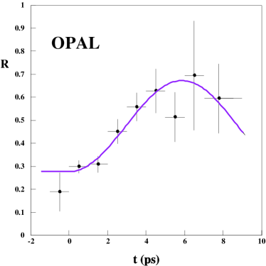
Figure 27: The ratio, R, of like-sign to total events as a function of proper decay time, for selected $B\to D^{*+}X\ell^{-}\bar{\nu}$ events. The jet charge in the opposite hemisphere is used to determine the sign correlation. The curve is the result of a fit to the mixing parameter.

Data from many experiments has been combined by “The LEP Working Group,” to obtain an average value $\Delta m_{d}=(0.489\pm 0.0008)\times 10^{12}\mbox{$h$\raisebox{-0.04303pt}{${}^{-}$}}$s^-1. Values from individual experiments are listed in Figure 28.

Figure 28: Values of the $B_{d}$ mixing parameter $\Delta m_{d}$ for each experiment.

The probability of mixing is given by (Gaillard 1974) (Bigi 2000)

$$x\equiv\frac{\Delta m}{\Gamma}={G_{F}^{2}\over 6\pi^{2}}B_{B}f_{B}^{2}m_{B}\tau_{B}|V^{*}_{tb}V_{td}|^{2}m_{t}^{2}F{\left(m^{2}_{t}\over M^{2}_{W}\right)}\eta_{QCD},$$ (45)

where $B_{B}$ is a parameter related to the probability of the $d$ and $\bar{b}$ quarks forming a hadron and must be estimated theoretically, $F$ is a known function which increases approximately as $m^{2}_{t}$, and $\eta_{QCD}$ is a QCD correction, with value about 0.8. By far the largest uncertainty arises from the unknown decay constant, $f_{B}$. In principle $f_{B}$ can be measured. The decay rate of the annihilation process $B^{-}\to\ell^{-}\overline{\nu}$ is proportional to the product of $f_{B}^{2}|V_{ub}|^{2}$. Even if $V_{ub}$ were well known this is a very difficult process to measure. Our current best hope is to rely on unquenched lattice QCD which can use the measurements of the analogous $D^{+}\to\mu^{+}\nu$ decay as check. This will take the construction of a “$\tau$-charm factory.”

Now we relate the mixing measurement to the CKM parameters. Since

$$|V^{*}_{tb}V_{td}|^{2}\propto|(1-\rho-i\eta)|^{2}=(\rho-1)^{2}+\eta^{2},$$ (46)

measuring mixing gives a circle centered at (1,0) in the $\rho-\eta$ plane. This could in principle be a very powerful constraint. Unfortunately, the parameter $B_{B}$ is not experimentally accessible and $f_{B}$, although in principle measurable, has not been and may not be for a very long time, so it too must be calculated. The errors on the calculations are quite large.

4.2 $B_{s}$ Mixing in the Standard Model

$B^{o}_{s}$ mesons can mix in a similar fashion to $B^{o}_{d}$ mesons. The diagrams in Figure 26 are modified by substituting $s$ quarks for $d$ quarks, thereby changing the relevant CKM matrix element from $V_{td}$ to $V_{ts}$. The time dependent mixing fraction is

$$x_{s}\equiv\frac{\Delta m_{s}}{\Gamma_{s}}={G_{F}^{2}\over 6\pi^{2}}B_{B_{s}}f_{B_{s}}^{2}m_{B_{s}}\tau_{B_{s}}|V^{*}_{tb}V_{ts}|^{2}m_{t}^{2}F{\left(m^{2}_{t}\over M^{2}_{W}\right)}\eta_{QCD},$$ (47)

which differs from equation (45) by having parameters relevant for the $B_{s}$ rather than the $B_{d}$.

Measuring $x_{s}$ allows us to use ratio of $x_{d}/x_{s}$ to provide constraints on the CKM parameters $\rho$ and $\eta$. We still obtain a circle in the ($\rho,\eta$) plane centered at (1,0):

$$\left|V_{td}\right|^{2} = A^{2}\lambda^{4}\left[(1-\rho)^{2}+\eta^{2}\right]$$ (48)

$${\left|V_{td}\right|^{2}\over\left|V_{ts}\right|^{2}} = (1-\rho)^{2}+\eta^{2}~{}~{}.$$

Now however we must calculate only the SU(3) broken ratios $B_{B_{d}}/B_{B_{s}}$ and $f_{B_{d}}/f_{B_{s}}$.

$B^{o}_{s}$ mixing has been searched for at LEP, the Tevatron, and the SLC. A combined analysis has been performed. The probability, ${\cal{P}}(t)$ for a $B_{s}$ to oscillate into a $\overline{B}_{s}$ is given as

$${\cal{P}}(t)\left(B_{s}\to\overline{B}_{s}\right)={1\over 2}\Gamma_{s}e^{-\Gamma_{s}t}\left[1+\cos\left(\Delta m_{s}t\right)\right]~{}~{},$$ (49)

where $t$ is the proper time.

To combine different experiments a framework has been established where each experiment finds a amplitude $A$ for each test frequency $\omega$, defined as

$${\cal{P}}(t)={1\over 2}\Gamma_{s}e^{-\Gamma_{s}t}\left[1+A\cos\left(\omega t\right)\right]~{}~{}.$$ (50)

Figure 29 shows the world average measured amplitude $A$ as a function of the test frequency $\omega=\Delta m_{s}$ (Leroy 2001). For each frequency the expected result is either zero for no mixing or one for mixing. No other value is physical, although allowing for measurement errors other values are possible. The data do indeed cross one at a $\Delta m_{s}$ of 16 ps^-1, however here the error on $A$ is about 0.6, precluding a statistically significant discovery. The quoted upper limit at 95% confidence level is 14.6 ps^-1. This is the point where the value of $A$ plus 1.645 times the error on $A$ reach one. Also indicated on the figure is the point where the error bar is small enough that a 4$\sigma$ discovery would be possible. This is at $\Delta m_{s}=11$ ps^-1. Also, one should be aware that all the points are strongly correlated.

The upper limit on $\Delta m_{s}$ translates to an upper limit on $x_{s}$ $<$21.6 also at 95% confidence level. CDF plans to probe higher sensitivity and eventually LHCb and BTeV can reach values of $\sim$80.

Figure 29: Combined experimental values of the amplitude $A$ versus the test frequency $\omega=\Delta m_{d}$ as defined in equation 50. The inner (outer) envelopes give the 95% confidence levels using statistical (statistical and systematic) errors. The “sensitivity” shown at 18.3 ps^-1 is the likely place a 95% c.l. upper limit could be set. Also indicated is the maximum value, 11 ps^-1, where a 4$\sigma$ discovery would be possible.

5 Rare $b$ Decays

5.1 Introduction

These processes proceed through higher order weak interactions involving loops, which are often called “Penguin” processes, for unscientific reasons (Lingel 1998). A Feynman loop diagram is shown in Figure 30 that describes the transition of a $b$ quark into a charged -1/3 $s$ or $d$ quark, which is effectively a neutral current transition. The dominant charged current decays change the $b$ quark into a charged +2/3 quark, either $c$ or $u$.

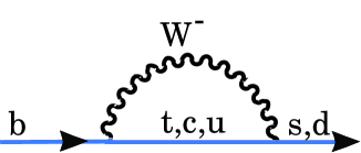
Figure 30: Loop or “Penguin” diagram for a $b\to s$ or $b\to d$ transition.

The intermediate quark inside the loop can be any charge +2/3 quark. The relative size of the different contributions arises from different quark masses and CKM elements. In terms of the Cabibbo angle ($\lambda$=0.22), we have for $t$:$c$:$u$ - $\lambda^{2}$:$\lambda^{2}$:$\lambda^{4}$. The mass dependence favors the $t$ loop, but the amplitude for $c$ processes can be quite large $\approx$30%. Moreover, as pointed out by Bander, Silverman and Soni (Bander 1979), interference can occur between $t$, $c$ and $u$ diagrams and lead to CP violation. In the Standard Model it is not expected to occur when $b\to s$, due to the lack of a CKM phase difference, but could occur when $b\to d$. In any case, it is always worth looking for this effect; all that needs to be done, for example, is to compare the number of $K^{*-}\gamma$ events with the number of $K^{*+}\gamma$ events.

There are other ways for physics beyond the Standard Model to appear. For example, the $W^{-}$ in the loop can be replaced by some other charged object such as a Higgs; it is also possible for a new object to replace the $t$.

5.2 Standard Model Theory

In the Standard Model the effective Hamiltonian for the intermediate $t$ quark is given by (Desphande 1994)

$$H_{eff}=-{{4G_{F}}\over\sqrt{2}}V_{tb}V_{ts}^{*}\sum_{i=1}^{10}C_{i}(\mu)O_{i}(\mu)~{}~{}.$$ (51)

Some of the more important operators are

$$O_{1}=\overline{s}_{L}^{i}\gamma_{\mu}b^{j}_{L}\overline{c}^{j}_{L}\gamma^{\mu}c^{j}_{L},~{}~{}~{}~{}O_{7}={e\over 16\pi^{2}}m_{b}\overline{s}_{L}^{i}\sigma_{\mu\nu}b_{R}^{j}F^{\mu\mu}~{}~{}.$$ (52)

The matrix elements are evaluated at the scale $\mu=M_{W}$ and then evolved to the $b$ mass scale using renormalization group equations, which mixes the operators:

$$C_{i}(\mu)=\sum_{j}U_{ij}(\mu,M_{W})C_{j}(M_{W})~{}~{}.$$ (53)

5.3 $b\to s\gamma$

This process occurs when any of the charged particles in Figure 30 emits a photon. The only operator which enters into the calculation is $C_{7}(\mu)$. We have for the inclusive decay

$$H_{eff} = {4G_{F}\over\sqrt{2}}\left(V_{tb}V_{ts}\right|^{2}C_{7}(m_{b})O_{7}$$ (54)

$$O_{7} = {e\over 16\pi^{2}}m_{b}\overline{s}_{L}\sigma_{\mu\nu}b_{R}F^{\mu\nu}$$ (55)

$$\Gamma(b\to s\gamma) = {{G_{F}^{2}\alpha m_{b}^{5}}\over 32\pi^{4}}\left|C_{7}\right|^{2}\left|V_{tb}V_{ts}^{*}\right|^{2}~{}~{}.$$ (56)

Its far more difficult to calculate the exclusive radiative decay rates, but they are much easier to measure. Note that the reaction $B\to K\gamma$ would violate angular momentum conservation, so the simplest exclusive final states are $B\to K^{*}\gamma$.

Different techniques are used for reconstructing exclusive and inclusive Decays and unique methods are invoked for exclusive decays on the $\Upsilon(4S)$. At other machines the decay products, $i$, from an exclusive $B$ decays are used to reconstruct an “invariant mass” via $M^{2}=\sum_{i}E_{i}^{2}-\sum_{i}\overrightarrow{p}_{\!i}^{2}$. At the $\Upsilon(4S)$ its done a bit differently, the decay products are first tested to see if the sum of their energies is close to the beam energy, $E_{beam}$. If this is true then the “beam constrained” invariant mass is calculated as $M^{2}=E_{beam}^{2}-\sum_{i}\overrightarrow{p}_{\!i}^{2}$. These methods are used for all exclusive $B$ decays, in combination with other requirements. Figure 31 shows the BELLE data for the reaction $\overline{B}^{o}\to D^{*+}\pi^{-}$, where the $D^{*+}\to\pi^{+}D^{o}$. BELLE first selects events with candidate $D^{o}$’s. Then they require an additional $\pi^{+}$ where the measured mass difference between the $D^{o}\pi^{+}$ minus the $D^{o}$ candidate is consistent with the known mass difference. Selecting the $D^{*+}$ candidates they combine them with candidate $\pi^{-}$. In Figure 31(a) the correlation between difference in measured energy $\Delta E=\sum_{i}E_{i}-E_{beam}$ versus the beam-constrained invariant mass is shown. In Figure 31(b) $\Delta E$ is shown after selecting the signal region in $M$ and in Figure 31(c) $M$ is shown after selecting on $\Delta E$. These plots show how clean signals can be selected.

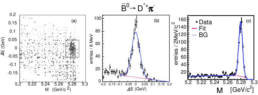
Figure 31: BELLE data for the reaction $\overline{B}^{o}\to D^{*+}\pi^{-}$. (a) The correlation between $\Delta E$ and $M$. The box shows the signal region. (b) The projection in $\Delta E$ for events in the $M$ signal region; the line shows a fit to the background. (c) The $M$ distribution for $\Delta E$ in the signal region; the line shows a fit to the background.

CLEO first measured the inclusive rate (Alam 1995) as well as the exclusive rate into $K^{*}(890)\gamma$ (Ammar 1993) shown in Figure 32. Here several different decay modes of the $K^{*}(890)$ are used. The current world average value for ${\cal{B}}(B\to K^{*}\gamma)=(4.2\pm 0.8\pm 0.6)\times 10^{-5}$.

Figure 32: First published CLEO data for the reaction ${B}\to K^{*}\gamma$ showing the $M$ distribution for $\Delta E$ in the signal region.

To find inclusive decays two techniques are used. The first one, which provides the cleanest signals, is to sum the exclusive decays for the final states $Kn\pi\gamma$, where $n\leq 4$ and only one of the pions is a $\pi^{o}$. These requirements are necessary or the backgrounds become extremely large. (Both charged and neutral kaons are used.) Of course, imposing these restrictions leads to a model dependence of the result that must be carefully evaluated. This is why having an independent technique is useful. That is provided by detecting only the high energy photon. The technique used is to form a neutral network to discriminate between continuum and $\Upsilon(4S)$ data using shape variables.

The momentum spectrum of the $\gamma$ peaks close to its maximum value at half the $B$ mass. If we had data with only $B$ mesons, it would be easy to pick out $b\to s\gamma$. We have, however, a large background from other processes. At the $\Upsilon(4S)$, the $\gamma$ spectrum from the different background processes is shown. The largest is $\pi^{o}$ production from continuum $e^{+}e^{-}$ collisions, but another large source is initial state radiation (ISR), where one of the beam electrons radiates a hard photon before annihilation. The backgrounds and the expected signal are illustrated in Figure 33. Similar backgrounds exist at LEP.

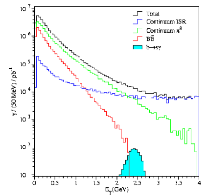
Figure 33: Levels of inclusive photons from various background processes at the $\Upsilon(4S)$ labeled largest to smallest at 2.5 GeV/c. Also shown is the expected signal from $b\to s\gamma$.

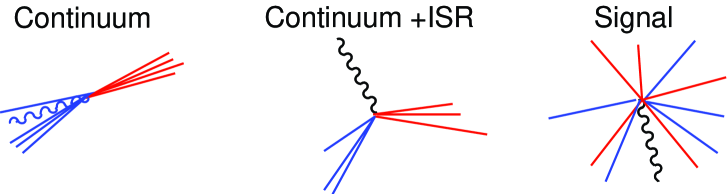
Figure 34: Examples of idealized event shapes. The straight lines indicate hadrons and the wavy lines photons.

To remove background CLEO used two techniques originally, one based on “event shapes” and the other on summing exclusively reconstructed $B$ samples. Examples of idealized events are shown in Figure 34. CLEO uses eight different shape variables described in Ref. [3], and defines a variable $r$ using a neural network to distinguish signal from background. The idea of the $B$ reconstruction analysis is to find the inclusive branching ratio by summing over exclusive modes. The allowed hadronic system is comprised of either a $K_{s}\to\pi^{+}\pi^{-}$ candidate or a $K^{\mp}$ combined with 1-4 pions, only one of which can be neutral. The restriction on the number and kind of pions maximizes efficiency while minimizing background. It does however lead to a model dependent error. For all combinations CLEO evaluates

$$\chi^{2}_{B}=\left({M_{B}-5.279}\over{\sigma_{M}}\right)^{2}+\left({E_{B}-E_{beam}}\over{\sigma_{E}}\right)^{2},$$ (57)

where $M_{B}$ is the measured $B$ mass for that hypothesis and $E_{B}$ is its energy. $\chi^{2}_{B}$ is required to be $<$ 20. If any particular event has more than one hypothesis, the solution which minimizes $\chi^{2}_{B}$ is chosen. For events with a reconstructed $B$ candidate CLEO also considers the angle between the direction of the $B$ and the thrust axis of event with the $B$ candidate removed, $\cos(\theta_{t})$. This is highly effective in removing continuum background.

A neural network is used to combine $r$, $\chi^{2}_{B}$, $\cos(\theta_{t})$ into a new variable $r_{c}$ and events are then weighted according to their value of $r_{c}$. This method maximizes the statistical potential of the data. Figure 35 shows the photon energy spectrum of the inclusive signal from CLEO combining both reconstruction techniques. The signal is compared to a theoretical prediction based on the model of Ali and Greub (Ali 1991). A fit to the model over the photon energy range from 2.0 to 2.7 GeV/c gives the branching ratio result shown in Table 5, where the first error is statistical, the second systematic and the third dependence on the theoretical model (Chen 2001).

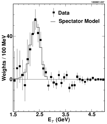
Figure 35: The background subtracted photon energy spectrum from CLEO. The spectrum is not corrected for resolution or efficiency. The solid lines show the spectrum from a simulation of the Ali-Greub spectator model with the $b$ quark mass set to 4.690 GeV and the Fermi momentum set to 410 MeV/c.

ALEPH reduces the backgrounds by weighting candidate decay tracks in a $b\to s\gamma$ event by a combination of their momentum, impact parameter with respect to the main vertex and rapidity with respect to the $b$-hadron direction (Barate 1998).

Current results are also shown in Table 5. The data are in agreement with the Standard Model theoretical prediction to next to leading order, including quark mass effects of $(3.73\pm 0.30)\times 10^{-4}$ (Hurth 2001). A deviation here would show physics beyond the Standard Model. More precise data and better theory are needed to further limit the parameter space of new physics models, or show an effect.

Table 5: ${\cal{B}}(b\to s\gamma)$.

Experiment	${\cal{B}}\times 10^{-4}$
CLEO	$3.21\pm 0.43\pm 0.27^{+0.18}_{-0.10}$
ALEPH	$3.11\pm 0.80\pm 0.72$
BELLE	$3.36\pm 0.53\pm 0.44^{+0.50}_{-0.54}$
Average	$3.23\pm 0.42$

5.3.1 $|V_{cb}|$ Using Moments of the Photon Energy Spectrum

In section(2.2.4) we found a value of $V_{cb}$ using the first and second hadronic mass moments. Here we use the first moment of the photon energy distribution in $b\to s\gamma$. The values found for the moments and $\overline{\Lambda}$ which is directly proportional to $\langle E_{\gamma}\rangle$ are (Chen 2001)

$$\langle E_{\gamma}\rangle = 2.346\pm 0.032\pm 0.011{~{}\rm GeV}$$ (58)

$$\langle E_{\gamma}^{2}\rangle-\langle E_{\gamma}\rangle^{2} = 0.0226\pm 0.0066\pm 0.0020{~{}\rm GeV^{2}}$$ (59)

$$\overline{\Lambda} = 0.35\pm 0.08\pm 0.10{~{}\rm GeV}.$$ (60)

In Figure 36 we show the combination of first moments from photon energy in $b\to s\gamma$ and hadron moments in $b\to c\ell\nu$. This implies a value of $V_{cb}$ around 0.0406.

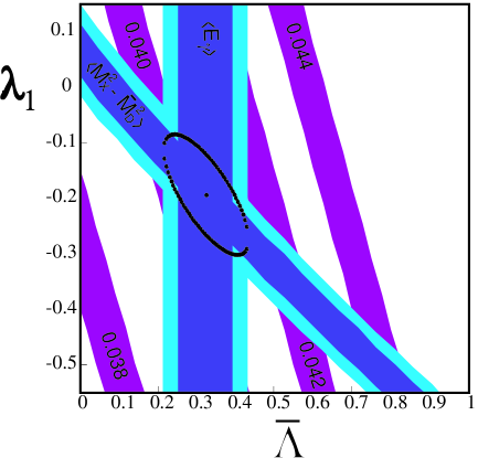
Figure 36: Correlation between $\lambda_{1}$, $\overline{\Lambda}$ and $V_{cb}$ derived from $\langle E_{\gamma}\rangle$ and $\langle M_{X}^{2}-\overline{M}_{D}^{2}\rangle$. The lighter bounds include both experimental and theoretical errors.

5.4 Rare Hadronic Decays

5.4.1 $B\to\pi\pi$ and $B\to K\pi$

The decays $\overline{B}^{o}\to\pi^{+}\pi^{-}$ and $\overline{B}^{o}\to K^{-}\pi^{+}$ do not contain any charm quarks in the final state so must proceed via either the tree level $V_{ub}$ process shown in Figure 37(left) or via the Penguin process shown on the right side.

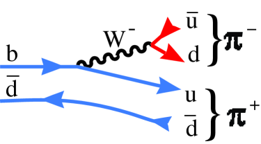
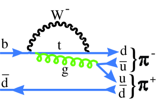
Figure 37: Decay diagrams for $\overline{B}^{o}\to\pi^{+}\pi^{-}$. (left) Via tree level $V_{ub}$ moderated decay. (right) Via a Penguin process.

These diagrams can interfere and they can also interfere through $B^{o}$ mixing, thus complicating any weak phase extraction. The same diagrams are applicable for $\overline{B}^{o}\to K^{-}\pi^{+}$ by replacing $W^{-}\to\bar{u}d$ in the tree level diagram by $W^{-}\to\bar{u}s$ and replacing the $td$ coupling in the Penguin by a $ts$ coupling.

Other diagrams for producing $K\pi$ final states are shown in Figure 38. In section 7.1 it will be shown that CP violation can result from the interference between two distinct decay amplitudes leading to the same final state. Consider the possibility of observing CP violation by measuring a rate difference between $B^{-}\to K^{-}\pi^{o}$ and $B^{+}\to K^{+}\pi^{o}$. The $K^{-}\pi^{o}$ final state can be reached either by tree or penguin diagrams.

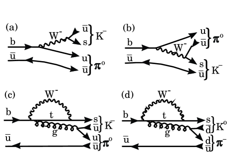
Figure 38: Diagrams for $B^{-}\to K^{-}\pi^{o}$, (a) and (b) are tree level diagrams where (b) is color suppressed; (c) is a penguin diagram. (d) shows $B^{-}\to K^{o}\pi^{-}$, which cannot be produced via a tree diagram.

The tree diagram has an imaginary part coming from the $V_{ub}$ coupling, while the penguin term does not, thus insuring a weak phase difference. This type of CP violation is called “direct.” Note also that the process $B^{-}\to K^{o}\pi^{-}$ can only be produced by the penguin diagram in Figure 38(d). Therefore, we do not expect a rate difference between $B^{-}\to K^{o}\pi^{-}$ and $B^{+}\to K^{o}\pi^{+}$.

Measurements of these rates have been by several groups. Recent data from BELLE are shown in Figure 39 (Abe 2001a). Table 6 lists the currently measured branching ratios.

Figure 39: Signals in $M$ and $\Delta E$ for two-body decay modes from BELLE. The data result from projections of a Likelihood fit that takes into account event shape and particle identification information. The dashed lines are the signal projections. The dotted lines in the $\Delta E$ distributions are projections of the background component from the $\pi\Leftrightarrow K$ substitution.

Table 6: Branching Ratios for $B\to K\pi$ and $B\to\pi\pi$ in units of $10^{-6}$.

Mode	CLEO	BABAR	BELLE	Average
$\pi^{+}\pi^{-}$	$4.7^{+1.8}_{-1.5}\pm 0.6$	$4.1\pm 1.0\pm 0.7$	$5.6^{+2.3}_{-2.0}\pm 0.4$	$4.5^{+0.9}_{-0.8}$
$\pi^{+}\pi^{o}$	$<$12	$<$9.6	$<$13.4
$K^{\pm}\pi^{\mp}$	$18.8^{+2.8}_{-2.6}\pm 1.3$	$16.7\pm 1.6\pm 1.3$	$19.3^{+3.4+1.5}_{-3.2-.06}$	$17.7^{+1.6}_{-1.5}$
$K^{+}\pi^{o}$	$12.1^{+3.0+2.1}_{-2.8-1.4}$	$10.8^{+2.1}_{-1.9}\pm 1.6$	$16.3^{+3.5+1.6}_{-3.3-1.8}$	$12.1^{+1.7}_{-1.6}$
$K^{o}\pi^{-}$	$18.2^{+4.6}_{-4.0}\pm 1.6$	$18.2^{+3.3}_{-3.0}\pm 2.0$	$13.7^{+5.7+1.9}_{-4.8-1.8}$	$17.3^{+2.7}_{-2.4}$
$K^{o}\pi^{o}$	$14.8^{+5.9+2.4}_{-5.1-3.3}$	$8.2^{+3.1}_{-2.7}\pm 1.2$	$16.0^{+7.2+2.5}_{-5.9-2.7}$	$10.4^{+2.7}_{-2.5}$

6 Hadronic Decays

6.1 Introduction

Mark Wise in his talk at the 2001 Lepton Photon conference (Wise 2001) gave some advice to theorists: “If you drink the nonlep tonic your physics career will be ruined and you will end up face down and in the gutter.” Presumably Mark’s statement was inspired by the difficulty in predicting hadronic decays. Here we have lots of gluon exchange with low energy gluons, while perturbation theory works well when the energies are large compared with $\Lambda_{QCD}$ $\sim$200 MeV. Furthermore, multibody decays are currently impossible to predict, so we will consider only two-body decays.

6.2 Two-Body Decays into a Charm or Charmonium

We start by considering two-body decays into a charmed hadron (Neubert 1997). Figure 6 shows the processes for both $B^{-}$ and $\overline{B}^{o}$ decays into a $D$ and a $\pi^{-}$. There is only one possible process for the $\overline{B}^{o}$, the simple spectator process (left), while the color suppressed spectator (right) is also allowed for the $B^{-}$. We call decays with only the simple spectator diagram allowed “class I” and decays where both the simple and color suppressed diagrams are allowed “class III.” Note, that because the colors of all the outgoing quarks must be the same in the color suppressed case, naively the amplitude is only $\sim$1/3 that of the simple spectator case where the $W^{-}$ can transform into quarks of all three colors. “Class II” decays are processes than can only be reached by the color suppressed spectator diagram, for example the $B^{o}\to J/\psi K_{s}$ decay shown in Figure 40.

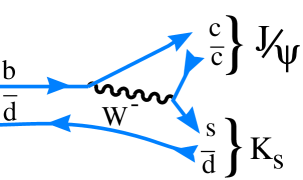
Figure 40: Color suppressed spectator decay diagram for $B^{o}\to J/\psi K_{s}$.

The effective Hamiltonian consists of local 4-quark operators renormalized at the scale $\mu$ and the Wilson coefficients (from the Operator Product Expansion) $c_{i}(\mu)$. We have

$$H_{eff} = {G_{F}\over\sqrt{2}}\left\{V_{cb}\left[c_{1}(\mu)Q_{1}^{cb}+c_{2}\mu)Q_{2}{cb}\right]+V_{ub}...\right\}$$ (61)

$$Q_{1}^{cb} = \left[(\overline{d}^{\prime}u)_{V-A}+(\overline{s}^{\prime}c)_{V-A}\right](\overline{c}^{\prime}b)_{V-A}$$

$$Q_{2}^{cb} = (\overline{c}u)_{V-A}(\overline{d}^{\prime}b)_{V-A}+(\overline{c}c)_{V-A}(\overline{s}^{\prime}b)_{V-A}~{}~{},$$

where the notation $(\overline{q_{1}}q_{2})_{V-A}\equiv\overline{q_{1}}\gamma_{\mu}(1-\gamma_{5})q_{2}$. Without QCD corrections $c_{1}(\mu)=1$ and $c_{2}(\mu)=0$. For non-leading order correction using the renormalization group equations, we have $c_{1}(\mu)=1.132$ and $c_{2}(\mu)=-0.249$.

We can factorize the amplitude by assuming that the current producing the $\pi^{-}$ is independent of the one producing the charmed hadron. Lets consider a class I case, $\overline{B}^{o}\to D^{+}\pi^{-}$. The amplitude can be written as

$$A_{fact}=-{G_{F}\over\sqrt{2}}V_{cb}V_{ud}^{*}{{a_{1}}}\langle\pi^{-}\left|(\overline{d}u)_{A}\right|0\rangle\langle D^{+}\left|(\overline{c}b)_{V}\right|\overline{B}^{o}\rangle$$ (62)

The part of the amplitude dealing with the $\pi^{-}$ is known from pion decay. We have $\langle\pi^{-}\left|\overline{d}\gamma_{\mu}\gamma_{5}u\right|0\rangle=if_{\pi}p_{\mu}$, where the axial vector structure is made explict, $p_{\mu}$ is the pion four-vector and $f_{\pi}$ is given by measuring the decay width for $\pi^{-}\to\mu^{-}\nu$. The term ${a_{1}}$ is defined as

$${a_{1}}=c_{1}(\mu_{f})+\xi c_{2}(\mu_{f})~{}~{},$$ (63)

where $\xi$ is equal to the number of colors and the scale $\mu_{f}$ is on the order of the $b$ quark mass. Then

$$A_{fact}=-{G_{F}\over\sqrt{2}}V_{cb}V_{ud}^{*}{{a_{1}}}f_{\pi}(m_{B}^{2}-m_{D}^{2})F_{0}^{B\to D}(m_{\pi}^{2})~{}~{}.$$ (64)

The $F_{0}$ form factor can either be calculated or measured, for example in semileptonic decays.

Let us also consider a class II process $B\to J/\psi K$. In this case

$$A_{fact}=-{G_{F}\over\sqrt{2}}V_{cb}V_{cs}^{*}{{a_{2}}}\langle J/\psi\left|(\overline{c}c)_{V}\right|0\rangle\langle K\left|(\overline{s}b)_{V}\right|{B}\rangle~{}~{},$$ (65)

where ${a_{2}}=c_{2}(\mu_{f})+\xi c_{1}(\mu_{f}).$

A class III decay has a term ${a_{1}}+x{a_{2}}$ in the amplitude, where $x$ equals one from flavor symmetry. However the actual values of ${a_{1}}$, $x$, and ${a_{2}}$ are not well predicted from theory but we can obtain them from the data.

One method is to use the class I decays to obtain ${a_{1}}=1.08\pm 0.04$. It is possible to calculate $a_{2}/a_{1}$ as shown in Figure 41 (Neubert 1997). Using these values the measured branching ratios are compared with the predicted ones in Table 7. Here $x=+1$ is used, taken from the data. This is opposite to the interference in $D$ decays but is expected from the calculation shown in Figure 41.

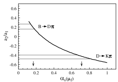
Figure 41: Calculated values of $a_{2}/a_{1}$ versus $\alpha_{s}$. The arrows indicate the ratios chosen for $B$ and $D$ decays.

Table 7: Predicted Branching Ratios ($10^{-4}$) (Neubert 1997) Compared to Measurement For Two-Body Hadronic Decays.

Class I			Class II			Class III
Mode	Model	Data	Mode	Model	Data	Mode	Model	Data
$D^{+}\pi^{-}$	30	30$\pm$4	$J/\psi K^{-}$	11	10$\pm$1	$D^{o}\pi^{-}$	48	53$\pm$5
$D^{*+}\pi^{-}$	30	28$\pm$2	$J/\psi K^{*}$	17	15$\pm$2	$D^{*o}\pi^{-}$	49	46$\pm$4
$D^{+}\rho^{-}$	70	79$\pm$14	$D^{o}\pi^{o}$	0.7	2.8$\pm$0.4	$D^{o}\rho^{-}$	110	134$\pm$18
$D^{*+}\rho^{-}$	85	73$\pm$15	$D^{*o}\pi^{o}$	1.0	2.1$\pm$0.9	$D^{*o}\rho^{-}$	119	155$\pm$31

The agreement is rather good except for the newly measured $D^{o(*)}\pi^{o}$ modes where it is rather miserable. CLEO and BELLE both have rates for $D^{o}\pi^{o}$ of $(2.7\pm 0.3\pm 0.5)\times 10^{-4}$ and $(2.9^{+0.4}_{-0.3}\pm 0.6)\times 10^{-4}$, respectively, while CLEO alone has measured $D^{*o}\pi^{o}$ as $(2.1\pm 0.5\pm 0.8)\times 10^{-4}$.

6.2.1 Isospin Analysis of the $B\to D\pi$ System

All the decay rates for $B\to D\pi$ have now been measured. The four-quark operator $(\overline{d}u)(\overline{c}b)$ has isospin I=1 and I₃=+1. It transforms the $\overline{B}^{o}$ into final states $D^{+}\pi^{-}$ and $D^{o}\pi^{o}$ with I=1/2 or I=3/2. The $B^{-}$ decays into $D^{o}\pi^{-}$ with I=3/2 only. It is thought that the isospin amplitudes cannot be modified by final state interactions, so we can look for evidence of final state phase shifts by doing an “isospin analysis.” The decay amplitudes form a triangle as shown in Figure 42.

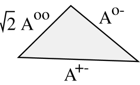
Figure 42: The isospin amplitude triangle for $B\to D\pi^{-}$ decays.

The relationship among $B$ decay amplitudes and isospin amplitudes is given by

$$A(\overline{B}^{o}\to D^{+}\pi^{-}) = \sqrt{1\over 3}A_{3/2}+\sqrt{2\over 3}A_{1/2}$$ (66)

$$A(\overline{B}^{o}\to D^{o}\pi^{o}) = \sqrt{2\over 3}A_{3/2}-\sqrt{1\over 3}A_{1/2}$$

$$A({B}^{-}\to D^{o}\pi^{-}) = \sqrt{3}A_{3/2}~{}~{}.$$

These equations may be solved for the isopsin amplitudes and the relative phase shift between the two amplitudes. The solution is

$$\left|A_{1/2}\right|^{2} = \left|A(\overline{B}^{o}\to D^{+}\pi^{-})\right|^{2}+\left|A(\overline{B}^{o}\to D^{o}\pi^{o})\right|^{2}-{1\over 3}\left|A({B}^{-}\to D^{o}\pi^{-})\right|^{2}$$ (67)

$$\left|A_{1/2}\right|^{2} = {1\over 3}\left|A({B}^{-}\to D^{o}\pi^{-})\right|^{2}$$

$$\cos\delta = \cos\left(\delta_{3/2}-\delta_{1/2}\right)={{3\left|A({B}^{-}\to D^{o}\pi^{-})\right|^{2}-2\left|A_{1/2}\right|^{2}-\left|A_{3/2}\right|^{2}}\over{2\sqrt{2}\left|A_{1/2}\right|\left|A_{3/2}\right|}}$$

Solving these equations for the $D\pi$ final states gives $\cos\delta=0.88\pm 0.05$ which indicates a phase shift of about $28\pm 8$ degrees, but is not statistically significant.

6.2.2 Factorization Tests Using Semileptonic Decays

The factorized amplitude for $D\pi^{-}$ decays in equation 65 is the product of two hadronic currents, one for $W^{-}\to\pi^{-}$ and the other for $B\to D$. In semileptonic decay (Figure 5) we have the product of the known lepton current and the pion current. At $q^{2}=m_{\pi}^{2}$ the $B\to D$ should be the same in both decays, at least for class I. The comparision for the general case of any hadron $h^{-}$ is

$$\left.\Gamma\left(\overline{B}\to D^{(*)}h\right)=6\pi^{2}a_{1}^{2}f_{h}^{2}\left|V_{ud}\right|^{2}{d\Gamma\over dq^{2}}\left(\overline{B}\to D^{(*)}\ell^{-}\overline{\nu}\right)\right|_{q^{2}=m_{h}^{2}}~{}~{}.$$ (68)

Tests of this equation for $D^{*+}$ and a $\pi^{-}$, $\rho^{-}$ or $a^{-}_{1}$ are satisfied at about 15% accuracy (Bortoletto 1990) (Browder 1996).

Another test compares the polarization of the $D^{*}$ in both hadronic and semileptonic cases:

$$\left.{\Gamma_{L}\over\Gamma}\left(\overline{B}\to D^{*}h\right)={\Gamma_{L}\over\Gamma}\left(\overline{B}\to D^{*}h\right)\right|_{q^{2}=m_{h}^{2}}~{}~{},$$ (69)

where $\Gamma_{L}$ denotes the longitudinally polarized fraction of the decay width. Comparisons with data will be shown in section 6.3.

There are also more modern approaches to factorization (Beneke 2001) (Bauer 2001). However these approaches predict

$${{\Gamma(B^{-}\to D^{o}\pi^{-})}\over{\Gamma(\overline{B}^{o}\to D^{+}\pi^{-})}}=1+{\cal O}(\Lambda_{QCD}/m_{b})~{}~{}$$ (70)

which seems to contradict current observations.

6.3 Observation of the $\rho^{\prime}$ in $B$ Decays

CLEO made the first statistically significant observations of six hadronic $B$ decays shown in Table 8 that result from studying the reactions $B\to D^{(*)}\pi^{+}\pi^{-}\pi^{-}\pi^{o}$ (Alexander 2001). The signal in one of these final states $\overline{B}^{o}\to D^{(*+)}\pi^{+}\pi^{-}\pi^{-}\pi^{o}$, where $D^{*+}\to\pi^{+}D^{o}$ and $D^{o}\to K^{-}\pi^{+}$ is shown in Figure 43.

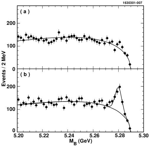
Figure 43: The $\overline{B}$ candidate mass spectra for the final state $D^{*+}\pi^{+}\pi^{-}\pi^{-}\pi^{0}$, with $D^{0}\to K^{-}\pi^{+}$ (a) for $\Delta E$ sidebands and (b) for $\Delta E$ consistent with zero. The curve in (a) is a fit to the background distribution described in the text, while in (b) the shape from (a) is used with the normalization allowed to float and a signal Gaussian of width 2.7 MeV is added.

In examining the substructure of the four-pions, a clear $\omega$ signal was observed in the $\pi^{+}\pi^{-}\pi^{o}$ mass as can be seen in Figure 44, leading to a significant amount of $D^{(*)}\omega\pi^{-}$. Furthermore, there is a low-mass resonant substructure in the $\omega\pi^{-}$ mass. (See Figure 45).

Table 8: Measured Branching Ratios

Mode	$\cal{B}$ (%)
$\overline{B}^{o}\to D^{*+}\pi^{+}\pi^{-}\pi^{-}\pi^{o}$	1.72$\pm$0.14$\pm$0.24
$\overline{B}^{o}\to D^{*+}\omega\pi^{-}$	0.29$\pm$0.03$\pm$0.04
$\overline{B}^{o}\to D^{+}\omega\pi^{-}$	0.28$\pm$0.05$\pm$0.03
${B}^{-}\to D^{*o}\pi^{+}\pi^{-}\pi^{-}\pi^{o}$	1.80$\pm$0.24$\pm$0.25
${B}^{-}\to D^{*o}\omega\pi^{-}$	0.45$\pm$0.10$\pm$0.07
${B}^{-}\to D^{o}\omega\pi^{-}$	0.41$\pm$0.07$\pm$0.04

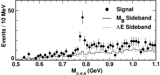
Figure 44: The invariant mass spectra of $\pi^{+}\pi^{-}\pi^{0}$ for the final state $D^{*+}\pi^{+}\pi^{-}\pi^{-}\pi^{0}$ for all three $D^{o}$ decay modes $K^{-}\pi^{+}$, $K^{-}\pi^{+}\pi^{+}\pi^{-}$ and $K^{-}\pi^{+}\pi^{o}$. The solid histogram is the background estimate from the $M_{B}$ lower sideband and the dashed histogram is from the $\Delta E$ sidebands; both are normalized to the fitted number of background events. (There is an additional cut selecting the center of the Dalitz plot.)

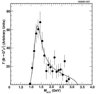
Figure 45: (left) The background subtracted efficiency corrected $\omega\pi^{-}$ mass spectrum from $\overline{B}^{o}\to(D^{*+}+D^{o}+D^{+})\omega\pi^{-}$ decays fit to a Breit-Wigner shape.

The spin and parity of the $\omega\pi^{-}$ resonance (denoted by $A$ temporarily) is determined by considering the decay sequence $B\rightarrow A\ D$; $A\rightarrow\omega\pi$ and $\omega\rightarrow\pi^{+}\pi^{-}\pi^{o}$. The angular distributions are shown in Figure 46. Here $\theta_{A}$ is the angle between the $\omega$ direction in the $A$ rest frame and the $A$ direction in the $B$ rest frame; $\theta_{\omega}$ is the orientation of the $\omega$ decay plane in the $\omega$ rest frame, and $\chi$ is the angle between the $A$ and $\omega$ decay planes.

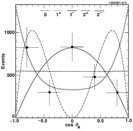
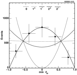
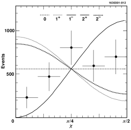
Figure 46: The angular distribution of $\theta_{A}$ (top-left),$\theta_{\omega}$ (top-right) and $\chi$ (bottom). The curves show the best fits to the data for for different $J^{P}$ assignments. The $0^{-}$ and $1^{+}$ are almost indistinguishable in $\cos\theta_{A}$, while the $1^{-}$ and $2^{+}$ are indistinguishable in $\cos\theta_{\omega}$ and $\chi$. The vertical axis gives efficiency corrected events, 104 events are used.

The data are fit to the expectations for the various $J^{P}$ assignments. The $\omega$ polarization is very clearly transverse ($\sin^{2}\theta_{\omega}$) and that infers a $1^{-}$ or $2^{+}$ assignment. The $\cos\theta_{A}$ distribution prefers $1^{-}$, as does the fit to all three projections.

This structure is identified with the $\rho^{\prime}$ because it has the correct $J^{P}$ and is at approximately the right mass. To determine the mass and width parameters, that are not well known, we write the decay width as a function of $\omega\pi^{-}$ mass as

$$d\Gamma(B\to D\omega\pi^{-}) = {1\over 2M_{B}}\left|A(B\to D\rho^{\prime})\cdot{\cal BW}(m_{\omega\pi})\cdot A(\rho^{\prime}\to\omega\pi^{-})\right|^{2}$$

$$\times dP(B\to D\rho^{\prime})\cdot dP(\rho^{\prime}\to\omega\pi^{-}){{dm^{2}_{\omega\pi}}\over 2\pi}~{}~{},$$

where $dP$ indicates phase space and the Breit-Wigner amplitude is given by

$${\cal BW}(m_{\omega\pi})={1\over{(m_{\omega\pi}^{2}-m_{\rho^{\prime}}^{2})-im_{\omega\pi}\Gamma_{tot}(m_{\omega\pi})}}~{}~{}.$$ (72)

The Breit-Wigner fit assuming a single resonance and no background gives a mass of 1349$\pm$25${}^{+10}_{-5}$ MeV with an intrinsic width of 547$\pm$86${}^{+46}_{-45}$ MeV. The fit shows that the $\omega\pi^{-}$ mass spectrum is consistent with being entirely one resonance. This state is likely to be the elusive $\rho^{\prime}$ resonance (Clegg 1994). These are by far the most accurate and least model dependent measurements of the $\rho^{\prime}$ parameters. The $\rho^{\prime}$ dominates the final state. (Thus the branching ratios for the $D^{(*)}\omega\pi^{-}$ apply also for $D^{(*)}\rho^{\prime-}$.)

Heavy quark symmetry predicts equal partial widths for $D^{*}\rho^{\prime}$ and$D\rho^{\prime}$. CLEO measures the relative rates to be ${{\Gamma\left({B}\to D^{*}\rho^{\prime-}\right)}/{\Gamma\left({B}\to D\rho^{\prime-}\right)}}=1.06\pm 0.17\pm 0.04$, consistent within the relatively large errors.

Factorization predicts that the fraction of longitudinal polarization of the $D^{*+}$ is the same as in the related semileptonic decay $B\to D^{*}\ell^{-}\bar{\nu}$ at four-momentum transfer $q^{2}$ equal to the mass-squared of the $\rho^{\prime}$

$${{\Gamma_{L}\left({B}\to D^{*+}\rho^{\prime-}\right)}\over{\Gamma\left({B}\to D^{*+}\rho^{\prime-}\right)}}={{\Gamma_{L}\left({B}\to D^{*}\ell^{-}\bar{\nu}\right)}\over{\Gamma\left({B}\to D^{*}\ell^{-}\bar{\nu}\right)}}\left|{}_{q^{2}=m^{2}_{\rho^{\prime}}}\right.~{}~{}.$$ (73)

CLEO’s measurement of the $D^{*+}$ polarization is (63$\pm$9)%. The model predictions in semileptonic decays for a $q^{2}$ of 2 GeV², are between 66.9 and 72.6% (Isgur 1990) (Wirbel 1985) (Neubert 1991). Figure 47 shows the measured polarizations for the $D^{*+}\rho^{\prime-}$, the $D^{*+}\rho^{-}$, (Artuso 1999) and the $D^{*+}D_{s}^{*-}$ final states (Stone 2000). The latter is based on a new measurement using partial reconstruction of the $D^{*+}$ (Ahmed 2000). Thus this prediction of factorization is satisfied.

Figure 47: Measured $D^{*+}$ polarization versus semileptonic model predictions.

7 CP Violation

7.1 Introduction

Recall that the operation of Charge Conjugation (C) takes particle to anti-particle and Parity (P) takes a vector $\overrightarrow{r}$ to $-\overrightarrow{r}$. CP violation can occur because of the imaginary term in the CKM matrix, proportional to $\eta$ in the Wolfenstein representation (Bigi 2000).

Consider the case of a process $B\to f$ that goes via two amplitudes A and B each of which has a strong part e. g. $s_{\cal{A}}$ and a weak part $w_{\cal{A}}$. Then we have

$$\Gamma(B\to f) = \left(\left|{\cal{A}}\right|e^{i(s_{\cal{A}}+w_{\cal{A}})}+\left|{\cal{B}}\right|e^{i(s_{\cal{B}}+w_{\cal{B}})}\right)^{2}$$ (74)

$$\Gamma(\overline{B}\to\overline{f}) = \left(\left|{\cal{A}}\right|e^{i(s_{\cal{A}}-w_{\cal{A}})}+\left|{\cal{B}}\right|e^{i(s_{\cal{B}}-w_{\cal{B}})}\right)^{2}$$ (75)

$$\Gamma(B\to f)-\Gamma(\overline{B}\to\overline{f}) = 2\left|{\cal{AB}}\right|\sin(s_{\cal{A}}-s_{\cal{B}})\sin(w_{\cal{A}}-w_{\cal{B}})~{}~{}.$$ (76)

Any two amplitudes will do, though its better that they be of approximately equal size. Thus charged $B$ decays can exhibit CP violation as well as neutral $B$ decays. In some cases, we will see that it is possible to guarantee that $\left|\sin(s_{\cal{A}}-s_{\cal{B}})\right|$ is unity, so we can get information on the weak phases. In the case of neutral $B$ decays, mixing can be the second amplitude.

7.2 Unitarity Triangles

The unitarity of the CKM matrix allows us to construct six relationships. The most useful turns out to be

$$V_{ud}V_{td}^{*}+V_{us}V_{ts}^{*}+V_{ub}V_{tb}^{*}=0~{}~{}.$$ (77)

To a good approximation

$$V_{ud}\approx V_{tb}^{*}\approx 1{\rm~{}~{}and~{}~{}}V_{ts}^{*}\approx-V_{cb},$$ (78)

then

$${V_{ub}\over V_{cb}}+{V_{td}^{*}\over V_{cb}}-V_{us}=0~{}~{}.$$ (79)

Since $V_{us}=\lambda$, we can define a triangle with sides

$$1$$ (80)

$$\left|{V_{td}\over A\lambda^{3}}\right| = {1\over\lambda}\sqrt{\left(\rho-1\right)^{2}+\eta^{2}}={1\over\lambda}\left|{V_{td}\over V_{ts}}\right|$$ (81)

$$\left|{V_{ub}\over A\lambda^{3}}\right| = {1\over\lambda}\sqrt{\rho^{2}+\eta^{2}}={1\over\lambda}\left|{V_{ub}\over V_{cb}}\right|.$$ (82)

The CKM triangle is depicted in Figure 48.

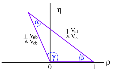
Figure 48: The unitarity triangle shown in the $\rho-\eta$ plane. The left side is determined by measurements of $b\to u/b\to c$ and the right side can be determined using mixing measurements in the $B_{s}$ and $B_{d}$ systems. The angles can be found by making measurements of CP violating asymmetries in hadronic $B$ decays.

We know the length of two sides already: the base is defined as unity and the left side is determined by the measurements of $|V_{ub}/V_{cb}|$, but the error is still quite substantial. The right side can be determined using mixing measurements in the neutral $B$ systems. Figure 48 also shows the angles as $\alpha,~{}\beta$, and $\gamma$. These angles can be determined by measuring CP violation in the $B$ system.

Another constraint on $\rho$ and $\eta$ is given by the $K_{L}^{o}$ CP violation measurement ($\epsilon$) (Buras 1995):

$$\eta\left[(1-\rho)A^{2}(1.4\pm 0.2)+0.35\right]A^{2}{B_{K}\over 0.75}=(0.30\pm 0.06),$$ (83)

where $B_{K}$ is parameter that cannot be measured and thus must be calculated. A reasonable range is $0.9>B_{k}>0.6$, given by an assortment of theoretical calculations (Buras 1995); this number is one of the largest sources of uncertainty. Other constraints come from current measurements on $V_{ub}/V_{cb}$, $B_{d}$ mixing and $B_{s}$ mixing. The current status of constraints on $\rho$ and $\eta$ is shown in Figure 49 (Hocker 2001). The width of both of these bands are also dominated by theoretical errors. This shows that the data are consistent with the standard model.

Figure 49: The regions in $\overline{\rho}-\overline{\eta}$ space (shaded), where $\overline{\rho}=\rho(1-\lambda^{2}/2)$ and $\overline{\eta}=\eta(1-\lambda^{2}/2)$, consistent with measurements of CP violation in $K_{L}^{o}$ decay ($\epsilon$), $V_{ub}/V_{cb}$ in semileptonic $B$ decay, $B_{d}^{o}$ mixing, and the excluded region from limits on $B_{s}^{o}$ mixing. The allowed region is defined by a fit from (Hocker 2001). The large width of the $B_{d}$ mixing band is dominated by the uncertainty in $B_{B}f_{B}^{2}$. The lines that are not specified are at 5% confidence level.

It is crucial to check if measurements of the sides and angles are consistent, i.e., whether or not they actually form a triangle. The standard model is incomplete. It has many parameters including the four CKM numbers, six quark masses, gauge boson masses and coupling constants. Perhaps measurements of the angles and sides of the unitarity triangle will bring us beyond the standard model and show us how these paramenters are related, or what is missing.

Furthermore, new physics can also be observed by measuring branching ratios which violate standard model predictions. Especially important are “rare decay,” processes such as $B\to K\mu^{+}\mu^{-}$ or $D\to\pi\mu^{+}\mu^{-}$. These processes occur only through loops, and are an important class of Penguin decays.

7.3 Formalism of CP Violation in Neutral $B$ Decays

Consider the operations of Charge Conjugation, C, and Parity, P:

$$C|B(\overrightarrow{p})\big{>}=|\overline{B}(\overrightarrow{p})\big{>},~{}~{}~{}~{}~{}~{}~{}~{}~{} C|\overline{B}(\overrightarrow{p})\big{>}=|{B}(\overrightarrow{p})\big{>}$$ (84)

$$P|B(\overrightarrow{p})\big{>}=-|{B}(-\overrightarrow{p})\big{>},~{}~{}~{}~{}~{} P|\overline{B}(\overrightarrow{p})\big{>}=-|\overline{B}(-\overrightarrow{p})\big{>}$$ (85)

$$CP|B(\overrightarrow{p})\big{>}=-|\overline{B}(-\overrightarrow{p})\big{>},~{}~{}~{} CP|\overline{B}(\overrightarrow{p})\big{>}=-|{B}(-\overrightarrow{p})\big{>}~{}~{}.$$ (86)

For neutral mesons we can construct the CP eigenstates

$$\big{|}B^{o}_{1}\big{>} = {1\over\sqrt{2}}\left(\big{|}B^{o}\big{>}-\big{|}\overline{B}^{o}\big{>}\right)~{}~{},$$ (87)

$$\big{|}B^{o}_{2}\big{>} = {1\over\sqrt{2}}\left(\big{|}B^{o}\big{>}+\big{|}\overline{B}^{o}\big{>}\right)~{}~{},$$ (88)

where

$$CP\big{|}B^{o}_{1}\big{>} = \big{|}B^{o}_{1}\big{>}~{}~{},$$ (89)

$$CP\big{|}B^{o}_{2}\big{>} = -\big{|}B^{o}_{2}\big{>}~{}~{}.$$ (90)

Since $B^{o}$ and $\overline{B}^{o}$ can mix, the mass eigenstates are a superposition of $a\big{|}B^{o}\big{>}+b\big{|}\overline{B}^{o}\big{>}$ which obey the Schrodinger equation

$$i{d\over dt}\left(\begin{array}[]{c}a\\ b\end{array}\right)={\cal H}\left(\begin{array}[]{c}a\\ b\end{array}\right)=\left(M-{i\over 2}\Gamma\right)\left(\begin{array}[]{c}a\\ b\end{array}\right).$$ (91)

If CP is not conserved then the eigenvectors, the mass eigenstates $\big{|}B_{L}\big{>}$ and $\big{|}B_{H}\big{>}$, are not the CP eigenstates but are

$$\big{|}B_{L}\big{>}=p\big{|}B^{o}\big{>}+q\big{|}\overline{B}^{o}\big{>},~{}~{}\big{|}B_{H}\big{>}=p\big{|}B^{o}\big{>}-q\big{|}\overline{B}^{o}\big{>},$$ (92)

where

$$p={1\over\sqrt{2}}{{1+\epsilon_{B}}\over{\sqrt{1+|\epsilon_{B}|^{2}}}},~{}~{}q={1\over\sqrt{2}}{{1-\epsilon_{B}}\over{\sqrt{1+|\epsilon_{B}|^{2}}}}.$$ (93)

CP is violated if $\epsilon_{B}\neq 0$, which occurs if $|q/p|\neq 1$.

The time dependence of the mass eigenstates is

$$\big{|}B_{L}(t)\big{>} = e^{-\Gamma_{L}t/2}e^{im_{L}t/2}\big{|}B_{L}(0)\big{>}$$ (94)

$$\big{|}B_{H}(t)\big{>} = e^{-\Gamma_{H}t/2}e^{im_{H}t/2}\big{|}B_{H}(0)\big{>},$$ (95)

leading to the time evolution of the flavor eigenstates as

$$\big{|}B^{o}(t)\big{>} = e^{-\left(im+{\Gamma\over 2}\right)t}\left(\cos{\Delta mt\over 2}\big{|}B^{o}(0)\big{>}+i{q\over p}\sin{\Delta mt\over 2}\big{|}\overline{B}^{o}(0)\big{>}\right)$$ (96)

$$\big{|}\overline{B}^{o}(t)\big{>} = e^{-\left(im+{\Gamma\over 2}\right)t}\left(i{p\over q}\sin{\Delta mt\over 2}\big{|}B^{o}(0)\big{>}+\cos{\Delta mt\over 2}\big{|}\overline{B}^{o}(0)\big{>}\right),$$ (97)

where $m=(m_{L}+m_{H})/2$, $\Delta m=m_{H}-m_{L}$ and $\Gamma=\Gamma_{L}\approx\Gamma_{H}$, and $t$ is the decay time in the $B^{o}$ rest frame, the so called proper time. Note that the probability of a $B^{o}$ decay as a function of $t$ is given by $\big{<}B^{o}(t)\big{|}B^{o}(t)\big{>}^{*}$, and is a pure exponential, $e^{-\Gamma t/2}$, in the absence of CP violation.

7.3.1 CP violation for $B$ via interference of mixing and decays

Here we choose a final state $f$ which is accessible to both $B^{o}$ and $\overline{B}^{o}$ decays (Bigi 2000). The second amplitude necessary for interference is provided by mixing. Figure 50 shows the decay into $f$ either directly or indirectly via mixing.

Figure 50: Two interfering ways for a $B^{o}$ to decay into a final state $f$.

It is necessary only that $f$ be accessible directly from either state; however if $f$ is a CP eigenstate the situation is far simpler. For CP eigenstates

$$CP\big{|}f_{CP}\big{>}=\pm\big{|}f_{CP}\big{>}.$$ (98)

It is useful to define the amplitudes

$$A=\big{<}f_{CP}\big{|}{\cal H}\big{|}B^{o}\big{>},~{}~{}\overline{A}=\big{<}f_{CP}\big{|}{\cal H}\big{|}\overline{B}^{o}\big{>}.$$ (99)

If $\left|{\overline{A}\over A}\right|\neq 1$, then we have “direct” CP violation in the decay amplitude, which we will discuss in detail later. Here CP can be violated by having

$$\lambda={q\over p}\cdot{\overline{A}\over A}\neq 1,$$ (100)

which requires only that $\lambda$ acquire a non-zero phase, i.e. $|\lambda|$ could be unity and CP violation can occur.

A comment on neutral $B$ production at $e^{+}e^{-}$ colliders is in order. At the $\Upsilon(4S)$ resonance there is coherent production of $B^{o}\bar{B}^{o}$ pairs. This puts the $B$’s in a $C=-1$ state. In hadron colliders, or at $e^{+}e^{-}$ machines operating at the $Z^{o}$, the $B$’s are produced incoherently. For the rest of this article I will assume incoherent production except where explicitly noted.

The asymmetry, in this case, is defined as

$$a_{f_{CP}}={{\Gamma\left(B^{o}(t)\to f_{CP}\right)-\Gamma\left(\overline{B}^{o}(t)\to f_{CP}\right)}\over{\Gamma\left(B^{o}(t)\to f_{CP}\right)+\Gamma\left(\overline{B}^{o}(t)\to f_{CP}\right)}},$$ (101)

which for $|q/p|=1$ gives

$$a_{f_{CP}}={{\left(1-|\lambda|^{2}\right)\cos\left(\Delta mt\right)-2{\rm Im}\lambda\sin(\Delta mt)}\over{1+|\lambda|^{2}}}.$$ (102)

For the cases where there is only one decay amplitude $A$, $|\lambda|$ equals 1, and we have

$$a_{f_{CP}}=-{\rm Im}\lambda\sin(\Delta mt).$$ (103)

Only the amplitude, ${\rm-Im}\lambda$ contains information about the level of CP violation, the sine term is determined only by $B_{d}$ mixing. In fact, the time integrated asymmetry is given by

$$a_{f_{CP}}=-{x\over{1+x^{2}}}{\rm Im}\lambda=-0.48{\rm Im}\lambda~{}~{}.$$ (104)

This is quite lucky as the maximum size of the coefficient for any $x$ is $-0.5$.

Let us now find out how ${\rm Im}\lambda$ relates to the CKM parameters. Recall $\lambda={q\over p}\cdot{\overline{A}\over A}$. The first term is the part that comes from mixing:

$${q\over p}={{\left(V_{tb}^{*}V_{td}\right)^{2}}\over{\left|V_{tb}V_{td}\right|^{2}}}={{\left(1-\rho-i\eta\right)^{2}}\over{\left(1-\rho+i\eta\right)\left(1-\rho-i\eta\right)}}=e^{-2i\beta}{\rm~{}~{}and}$$ (105)

$${\rm Im}{q\over p}=-{{2(1-\rho)\eta}\over{\left(1-\rho\right)^{2}+\eta^{2}}}=\sin(2\beta).$$ (106)

To evaluate the decay part we need to consider specific final states. For example, consider $f\equiv\pi^{+}\pi^{-}$. The simple spectator decay diagram is shown in Figure 37 (left). For the moment we will assume that this is the only diagram which contributes, which we know is not true. For this $b\to u\bar{u}d$ process we have

$${\overline{A}\over A}={{\left(V_{ud}^{*}V_{ub}\right)^{2}}\over{\left|V_{ud}V_{ub}\right|^{2}}}={{(\rho-i\eta)^{2}}\over{(\rho-i\eta)(\rho+i\eta)}}=e^{-2i\gamma},$$ (107)

and

$${\rm Im}(\lambda)={\rm Im}(e^{-2i\beta}e^{-2i\gamma})={\rm Im}(e^{2i\alpha})=-\sin(2\alpha).$$ (108)

For our next example let’s consider the final state $J/\psi K_{s}$. The decay diagram is shown in Figure 40. In this case we do not get a phase from the decay part because

$${\overline{A}\over A}={{\left(V_{cb}V_{cs}^{*}\right)^{2}}\over{\left|V_{cb}V_{cs}\right|^{2}}}$$ (109)

is real to order $1/\lambda^{4}$.

In this case the final state is a state of negative $CP$, i.e. $CP\big{|}J/\psi K_{s}\big{>}=-\big{|}J/\psi K_{s}\big{>}$. This introduces an additional minus sign in the result for ${\rm Im}\lambda$. Before finishing discussion of this final state we need to consider in more detail the presence of the $K_{s}$ in the final state. Since neutral kaons can mix, we pick up another mixing phase (similar diagrams as for $B^{o}$, see Figure 26). This term creates a phase given by

$$\left({q\over p}\right)_{K}={{\left(V_{cd}^{*}V_{cs}\right)^{2}}\over{\left|V_{cd}V_{cs}\right|^{2}}},$$ (110)

which is real to order $\lambda^{4}$. It necessary to include this term, however, since there are other formulations of the CKM matrix than Wolfenstein, which have the phase in a different location. It is important that the physics predictions not depend on the CKM convention.

In summary, for the case of $f=J/\psi K_{s}$, ${\rm Im}\lambda=-\sin(2\beta)$.

7.3.2 Comment on Penguin Amplitude

In principle all processes can have penguin components. One such diagram is shown in Figure 37(right). The $\pi^{+}\pi^{-}$ final state is expected to have a rather large penguin amplitude $\sim$10% of the tree amplitude. Then $|\lambda|\neq 1$ and $a_{\pi\pi}(t)$ develops a $\cos(\Delta mt)$ term. It turns out that $\sin(2\alpha)$ can be extracted using isospin considerations and measurements of the branching ratios for $B^{+}\to\pi^{+}\pi^{o}$ and $B^{o}\to\pi^{o}\pi^{o}$, or other methods the easiest of which appears to be the study of $B^{o}\to\rho\pi$.

In the $J/\psi K_{s}$ case, the penguin amplitude is expected to be small since a $c\bar{c}$ pair must be “popped” from the vacuum. Even if the penguin decay amplitude were of significant size, the decay phase is the same as the tree level process, namely zero.

7.4 Results on $\sin{2\beta}$

For years observation of large CP violation in the $B$ system was considered to be one of the corner stone predictions of the Standard Model. Yet it took a very long time to come up with definitive evidence. The first statistically significant measurements of CP violation in the $B$ system were made recently by BABAR and BELLE. This enormous achievement was accomplished using an asymmetric $e^{+}e^{-}$ collider on the $\Upsilon(4S)$ which was first suggested by Pierre Oddone. The measurements are listed in Table 9, along with other previous indications (Groom 2001).

Table 9: Measurements of $\sin 2\beta$.

Experiment	$\sin 2\beta$
BABAR	$0.59\pm 0.14\pm 0.05$
BELLE	$0.99\pm 0.14\pm 0.06$
Average	0.79$\pm$0.11
CDF	0.79${}^{+.41}_{-0.44}$
ALEPH	0.84${}^{+0.82}_{-1.04}\pm 0.16$
OPAL	3.2${}^{+1.8}_{-2.0}\pm 0.5$

The average value of $0.79\pm 0.11$ is taken from BABAR and BELLE only. These two measurements do differ by a sizeable amount, but the confidence level that they correctly represent the same value is 6%. This value is consistent with what is expected from the other known constraints on $\rho$ and $\eta$. We have

$$\overline{\eta}=(1-\overline{\rho}){{1\pm\sqrt{1-\sin^{2}{2\beta}}}\over\sin{2\beta}}~{}~{}.$$ (111)

There is a four fold ambiguity in the translation between $\sin{2\beta}$ and the linear constraints in the $\rho-\eta$ plane. These occur at $\beta$, $\pi/2-\beta$, $\pi+\beta$ and $3\pi/2-\beta.$ Two of these constraints are shown in Figure 51. The other two can be viewed by extending these to negative $\overline{\eta}$. We think $\eta>0$ based only on measurement of $\epsilon^{\prime}$ in the neutral kaon system.

Figure 51: Constraints from $\sin 2\beta$ measurement overlaid with other constraints (Hocker 2001). The inner band is at 1$\sigma$ while the outer band, shown on one band only, is at $2\sigma$.

7.5 Remarks on Global Fits to CKM parameters

The fits shown in this paper (Hocker 2001) for $\rho$ and $\eta$ have been done by others with a somewhat different statistical framework (Ciuchini 2001) (Mele 1999). The latter group uses “Bayesian” statistics which means that they use apriori knowledge of the probability distribution functions. The former are termed “frequentists” (Groom 2001), almost for the lack of a better term. The frequentists are more conservative than the Bayesians.

The crux of the issue is how to treat theoretically predicted parameters that are used to translate measurements into quantities such as $V_{ub}$ or $\epsilon_{K}$ that form constraints in the $\rho-\eta$ plane. This of course is a problem because it is difficult to estimate the uncertainties in the theoretical predictions. Both groups treat the experimental measurements as Gaussian distributions with the $1\sigma$ width derived from both the statistical and systematic errors combined. Note, that the systematic errors are also difficult sometimes to quantify and are not necessarily Gaussian, but they judged to be sufficiently well known as to not cause a problem.

Hocker et al. (Hocker 2001) have decided to use a method which restricts the theoretical quantities to a 95% confidence interval where the parameter in question is just as likely to lie anywhere in the interval. They call this the “Rfit” method. Of course assigning the 95% confidence interval is a matter of judgment which they fully admit. Ciuchini et al. (Ciuchini 2001) treat the theoretical errors in the same manner as the experimental errors. They call theirs “the standard method” with just a bit of hubris. They argue that QCD is mature enough to trust its predictions, that they know the sign and rough magnitude of corrections and they can assign reasonable errors, so it would be wrong to throw away information.

Hocker et al. point out an extreme interesting but generally unknown danger with the Bayesian approach, which is that in multi-dimension problems the Bayesian treatment unfairly predicts a narrowing of possible results. The following discussion will demonstrate this.

Let $x_{i}$ denote N theoretical parameters over the identical ranges $[-\Delta,+\Delta]$; then the theoretical prediction is

$$T_{P}^{(N)}=\prod_{i}^{N}x_{i}~{}~{}.$$ (112)

In the 95% scan scheme $[T^{(N)}_{P}]=[-\Delta^{N},+\Delta^{N}]$ while in the Bayesian approach the convoluted Probability Density Function (PDF) is

$$\rho(T)=\int_{-\infty}^{+\infty}...\int_{-\infty}^{+\infty}\prod_{i}^{N}dx_{i}G(x_{i})\delta(T-T_{P}^{(N)})~{}~{},$$ (113)

where the $G(x_{i})$ are PDF’s for each individual variable taken to be equal here. This function has a singularity in $\rho(T)$ that goes as $(-lnT)^{N-1}$, so it increases as $N$ increases.

Now suppose $G(x_{i})$ is flat, then for $N=1$ both approaches are the same, but for $N\geq 2$, the Bayesian approach gets a $\rho(T)$ that peaks at zero. In effect, when the number of theoretical predictions entering the computation increases, and hence our knowledge of the corresponding observable decrease the Bayesian approach claims the converse.

Lets look at a specific example: here $N=3$ and $\Delta=\sqrt{3}$. Consider both the sum $T_{S}=x_{1}+x_{2}+x_{3}$ and product $T_{P}=x_{1}x_{2}x_{3}$ distributions. For Rfit the allowed ranges are identical being $[-3\Delta,3\Delta]$. The left side of Figure 52 shows the probability density $\rho(T)$ for $T_{S}$, while the right side shows $\rho(T)$ for $T_{P}$ with $G(x)$ in the Bayesian case being either a Gaussian with $\sigma=1$ (solid lines) or a uniform distribution over the range $[-\sqrt{3},+\sqrt{3}]$ (dashed lines). The later distribution is closest to the Rfit method where the allowed range for either $T$ is $[-3\sqrt{3},+3\sqrt{3}]$ indicated by the arrows.

In the Rfit scheme the two predictions for $T_{P}$ and $T_{S}$ are identical, while in the Bayesian scheme there is large difference in the PDF’s and it really doesn’t matter if a Gaussian or uniform distribution is chosen. There is a clear distinction between the Rfit and Bayesian predictions for $T_{P}$ in this case, and the Bayesian one is unreasonable because it produces a very narrow PDF peaked very close to zero.

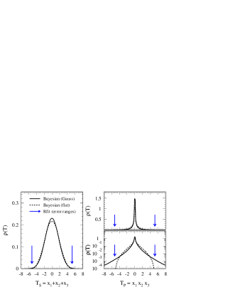
Figure 52: Convolution of the sum $T_{S}=x_{1}+x_{2}+x_{3}$ for both Rfit and Bayesian methods (left) and the product $T_{P}=x_{1}x_{2}x_{3}$ (right) of 3 parameters for the Bayesian method only. Plotted is the PDF $\rho(T)$ obtained using for $G(x)$ a uniform (solid lines, $\Delta=\sqrt{3}$) or a Gaussian (dashed lines, $\sigma=1$) distribution. Both PDF’s of $T_{P}$ have a singularity at the origin which is not shown. The Rfit ranges of $T_{S}$ and $T_{P}$ are indicated by the arrows located in both instances at $\pm 3\sqrt{3}$. From (Hocker 2001).

An example of how this can effect the results is shown on Figure 53 where predictions of $\sin 2\beta$ from the indirect measurements are shown for the Rfit technique and either uniform or Gaussian Bayesian PDF’s. The predictions are quite different.

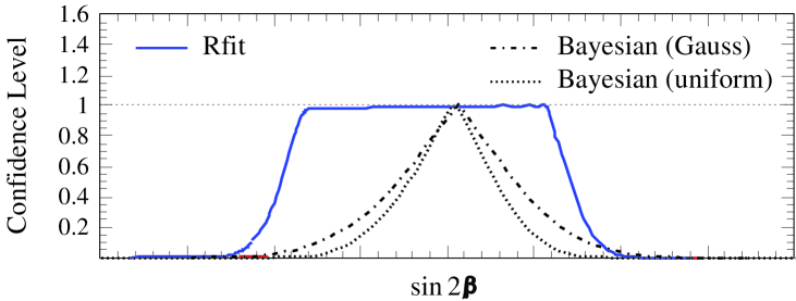
Figure 53: Comparison between Rfit (broad solid curve) and Bayesian fits for the indirect CKM constraints on $\sin 2\beta$. For the Bayesian fits: Gaussian (uniform) theoretical PDF’s are depicted as dashed-dotted (dotted) curves. (This example has been outdated by newer data.)

8 New Physics Studies

8.1 Introduction

There are many reasons why we believe that the Standard Model is incomplete and there must be physics beyond. One is the plethora of “fundamental parameters,” for example quark masses, mixing angles, etc… The Standard Model cannot explain the smallness of the weak scale compared to the GUT or Planck scales; this is often called “the hierarchy problem.” In the Standard Model it is believed that the CKM source of CP violation extensively discussed here is not large enough to explain the baryon asymmetry of the Universe (Gavela 1993); we can also take the view that we will discover additional large unexpected effects in $b$ and/or $c$ decays. Finally, gravity is not incorporated. John Ellis said “My personal interest in CP violation is driven by the search for physics beyond the Standard Model” (Ellis 2000).

We must realize that all our current measurements are a combination of Standard Model and New Physics; any proposed models must satisfy current constraints. Since the Standard Model tree level diagrams are probably large, lets consider them a background to New Physics. Therefore loop diagrams and CP violation are the best places to see New Physics.

The most important current constraints on New Physics models are

• The neutron electric dipole moment, $d_{N}~{}<6.3\times 10^{-26}$e-cm.

• ${\cal{B}}(b\to s\gamma)=(3.23\pm 0.42)\times 10^{-4}$ and ${\cal{B}}(b\to s\ell^{+}\ell^{-})<4.2\times 10^{-5}$.

• CP violation in $K_{L}$ decay, $\epsilon_{K}=(2.271\pm 0.017)\times 10^{-3}$.

• $B^{o}$ mixing parameter $\Delta m_{d}=(0.487\pm 0.014)$ ps^-1.

8.2 Generic Tests for New Physics

We can look for New Physics either in the context of specific models or more generically, for deviations from the Standard Model expectation.

One example is to examine the rare decays $B\to K\ell^{+}\ell^{-}$ and $B\to K^{*}\ell^{+}\ell^{-}$ for branching ratios and polarizations. According to Greub et al., “Especially the decay into $K^{*}$ yields a wealth of new information on the form of the new interactions since the Dalitz plot is sensitive to subtle interference effects” (Greub 1995).

Another important tactic is to test for inconsistencies in Standard Model predictions independent of specific non-standard models.

The unitarity of the CKM matrix allows us to construct six relationships. These may be thought of as triangles in the complex plane shown in Figure 54. (The bd triangle is the one depicted in Figure 48.)

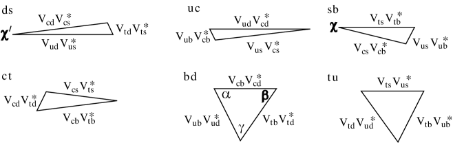
Figure 54: The six CKM triangles. The bold labels, e.g. ds refer to the rows or columns used in the unitarity relationship. The angles defined in equation (114) are also shown.

All six of these triangles can be constructed knowing four and only four independent angles (Silva 1997) (Aleksan 1994). These are defined as:

$$\beta=arg\left(-{V_{tb}V^{*}_{td}\over V_{cb}V^{*}_{cd}}\right), \gamma=arg\left(-{{V^{*}_{ub}V_{ud}}\over{V^{*}_{cb}V_{cd}}}\right),$$ (114)

$$\chi=arg\left(-{V^{*}_{cs}V_{cb}\over V^{*}_{ts}V_{tb}}\right), \chi^{\prime}=arg\left(-{{V^{*}_{ud}V_{us}}\over{V^{*}_{cd}V_{cs}}}\right).$$

($\alpha$ can be used instead of $\gamma$ or $\beta$.) Two of the phases $\beta$ and $\gamma$ are probably large while $\chi$ is estimated to be small $\approx$0.02, but measurable, while $\chi^{\prime}$ is likely to be much smaller.

It has been pointed out by Silva and Wolfenstein (Silva 1997) that measuring only angles may not be sufficient to detect new physics. For example, suppose there is new physics that arises in $B^{o}-\overline{B}^{o}$ mixing. Let us assign a phase $\theta$ to this new physics. If we then measure CP violation in $B^{o}\to J/\psi K_{s}$ and eliminate any Penguin pollution problems in using $B^{o}\to\pi^{+}\pi^{-}$, then we actually measure $2\beta^{\prime}=2\beta+\theta$ and $2\alpha^{\prime}=2\alpha-\theta$. So while there is new physics, we miss it, because $2\beta^{\prime}+2\alpha^{\prime}=2\alpha+2\beta$ and $\alpha^{\prime}+\beta^{\prime}+\gamma=180^{\circ}$.

8.2.1 A Critical Check Using $\chi$

The angle $\chi$, defined in equation 114, can be extracted by measuring the time dependent CP violating asymmetry in the reaction $B_{s}\to J/\psi\eta^{(}$^′), or if one’s detector is incapable of quality photon detection, the $J/\psi\phi$ final state can be used. However, in this case there are two vector particles in the final state, making this a state of mixed CP, requiring a time-dependent angular analysis to extract $\chi$, that requires large statistics.

Measurements of the magnitudes of CKM matrix elements all come with theoretical errors. Some of these are hard to estimate. The best measured magnitude is that of $\lambda=|V_{us}/V_{ud}|=0.2205\pm 0.0018$.

Silva and Wolfenstein (Silva 1997) (Aleksan 1994) show that the Standard Model can be checked in a profound manner by seeing if:

$$\sin\chi=\left|{V_{us}\over V_{ud}}\right|^{2}{{\sin\beta~{}\sin\gamma}\over{\sin(\beta+\gamma)}}~{}~{}.$$ (116)

Here the precision of the check will be limited initially by the measurement of $\sin\chi$, not of $\lambda$. This check can reveal new physics, even if other measurements have not shown any anomalies.

Other relationships to check include:

$$\sin\chi=\left|{V_{ub}\over V_{cb}}\right|^{2}{\sin\gamma~{}\sin(\beta+\gamma)\over{\sin\beta}}~{}~{},$$ (117)

$$\sin\chi=\left|{V_{td}\over V_{ts}}\right|^{2}{\sin\beta~{}\sin(\beta+\gamma)\over{\sin\gamma}}~{}~{}.$$ (118)

The astute reader will have noticed that these two equations lead to the non-trivial relationship:

$$\sin^{2}\beta\left|V_{td}\over V_{ts}\right|^{2}=\sin^{2}\gamma\left|{V_{ub}\over V_{cb}}\right|^{2}~{}~{}.$$ (119)

This constrains these two magnitudes in terms of two of the angles. Note, that it is in principle possible to determine the magnitudes of $|V_{ub}/V_{cb}|$ and $|V_{td}/V_{ts}|$ without model dependent errors by measuring $\beta$, $\gamma$ and $\chi$ accurately. Alternatively, $\beta$, $\gamma$ and $\lambda$ can be used to give a much more precise value than is possible at present with direct methods. For example, once $\beta$ and $\gamma$ are known

$$\left|{V_{ub}\over V_{cb}}\right|^{2}=\lambda^{2}{{\sin^{2}\beta}\over{\sin^{2}(\beta+\gamma)}}~{}~{}~{}.$$ (120)

Table 10 lists the most important physics quantities and the decay modes that can be used to measure them. The necessary detector capabilities include the ability to collect purely hadronic final states labeled here as “Hadron Trigger,” the ability to identify charged hadrons labeled as “$K\pi$ sep,” the ability to detect photons with good efficiency and resolution and excellent time resolution required to analyze rapid $B_{s}$ oscillations. Measurements of $\cos(2\phi)$ can eliminate 2 of the 4 ambiguities in $\phi$ that are present when $\sin(2\phi)$ is measured.

Physics	Decay Mode	Hadron	$K\pi$	$\gamma$	Decay
Quantity		Trigger	sep	det	time $\sigma$
$\sin(2\alpha)$	$B^{o}\to\rho\pi\to\pi^{+}\pi^{-}\pi^{o}$	$\surd$	$\surd$	$\surd$
$\cos(2\alpha)$	$B^{o}\to\rho\pi\to\pi^{+}\pi^{-}\pi^{o}$	$\surd$	$\surd$	$\surd$
sign$(\sin(2\alpha))$	$B^{o}\to\rho\pi$ & $B^{o}\to\pi^{+}\pi^{-}$	$\surd$	$\surd$	$\surd$
$\sin(\gamma)$	$B_{s}\to D_{s}^{\pm}K^{\mp}$	$\surd$	$\surd$		$\surd$
$\sin(\gamma)$	$B^{-}\to\overline{D}^{0}K^{-}$	$\surd$	$\surd$
$\sin(\gamma)$	$B^{o}\to\pi^{+}\pi^{-}$ & $B_{s}\to K^{+}K^{-}$	$\surd$	$\surd$		$\surd$
$\sin(2\chi)$	$B_{s}\to J/\psi\eta^{\prime},$ $J/\psi\eta$			$\surd$	$\surd$
$\sin(2\beta)$	$B^{o}\to J/\psi K_{s}$
$\cos(2\beta)$	$B^{o}\to J/\psi K^{o}$, $K^{o}\to\pi\ell\nu$		$\surd$
$\cos(2\beta)$	$B^{o}\to J/\psi K^{*o}$ & $B_{s}\to J/\psi\phi$
$x_{s}$	$B_{s}\to D_{s}^{+}\pi^{-}$	$\surd$			$\surd$
$\Delta\Gamma$ for $B_{s}$	$B_{s}\to J/\psi\eta^{\prime}$, $D_{s}^{+}\pi^{-}$, $K^{+}K^{-}$	$\surd$	$\surd$	$\surd$	$\surd$

Table 10: Required CKM Measurements for $b$’s

8.2.2 Finding Inconsistencies

Another interesting way of viewing the physics was given by Peskin (Peskin 2000). Non-Standard Model physics would show up as discrepancies among the values of $(\rho,\eta)$ derived from independent determinations using CKM magnitudes ($|V_{ub}/V_{cb}|$ and $|V_{td}/V_{ts}|$), or $B^{o}_{d}$ mixing ($\beta$ and $\alpha$), or $B_{s}$ mixing ($\chi$ and $\gamma$).

8.2.3 Required Measurements Involving $\beta$

Besides a more precise measurement of $\sin 2\beta$ we need to resolve the ambiguities. There are two suggestions on how this may be accomplished. Kayser (Kayser 1997) shows that time dependent measurements of the final state $J/\psi K^{o}$, where $K^{o}\to\pi\ell\nu$, give a direct measurement of $\cos(2\beta)$ and can also be used for CPT tests. Another suggestion is to use the final state $J/\psi K^{*o}$, $K^{*o}\to K_{s}\pi^{o}$, and to compare with $B_{s}\to J/\psi\phi$ to extract the sign of the strong interaction phase shift assuming SU(3) symmetry, and thus determine $\cos(2\beta)$ (Dighe 1998).

8.2.4 Required Measurements Involving $\alpha$ and $\gamma$

It is well known that $\sin(2\beta)$ can be measured without problems caused by Penguin processes using the reaction $B^{o}\to J/\psi K_{s}$. The simplest reaction that can be used to measure $\sin(2\alpha)$ is $B^{o}\to\pi^{+}\pi^{-}$. This reaction can proceed via both the Tree and Penguin diagrams shown in Figure 37.

Current measurements shown in Table 6 show a large Penguin component. The ratio of Penguin amplitude to Tree amplitude in the $\pi^{+}\pi^{-}$ channel is about 15% in magnitude. Thus the effect of the Penguin must be determined in order to extract $\alpha$. The only model independent way of doing this was suggested by Gronau and London, but requires the measurement of $B^{\mp}\to\pi^{\mp}\pi^{o}$ and $B^{o}\to\pi^{o}\pi^{o}$, the latter being rather daunting.

There is however, a theoretically clean method to determine $\alpha$. The interference between Tree and Penguin diagrams can be exploited by measuring the time dependent CP violating effects in the decays $B^{o}\to\rho\pi\to\pi^{+}\pi^{-}\pi^{o}$ as shown by Snyder and Quinn (Snyder 1993).

The $\rho\pi$ final state has many advantages. First of all, it has been seen with a relatively large rate. The branching ratio for the $\rho^{o}\pi^{+}$ final state as measured by CLEO is $(1.5\pm 0.5\pm 0.4)\times 10^{-5}$, and the rate for the neutral $B$ final state $\rho^{\pm}\pi^{\mp}$ is $(3.5^{+1.1}_{-1.0}\pm 0.5)\times 10^{-5}$, while the $\rho^{o}\pi^{o}$ final state is limited at 90% confidence level to $<5.1\times 10^{-6}$ (Gao 1999). (BABAR (Bona 2001) measures ${\cal{B}}\left(B^{o}\to\rho^{\pm}\pi^{\mp}\right)$ as $(28.9\pm 5.4\pm 4.3)\times 10^{-6}$.) These measurements are consistent with some theoretical expectations (Ali 1999). Furthermore, the associated vector-pseudoscalar Penguin decay modes have conquerable or smaller branching ratios. Secondly, since the $\rho$ is spin-1, the $\pi$ spin-0 and the initial $B$ also spinless, the $\rho$ is fully polarized in the (1,0) configuration, so it decays as $\cos^{2}\theta$, where $\theta$ is the angle of one of the $\rho$ decay products with the other $\pi$ in the $\rho$ rest frame. This causes the periphery of the Dalitz plot to be heavily populated, especially the corners. A sample Dalitz plot is shown in Figure 55. This kind of distribution is good for maximizing the interferences, which helps minimize the error. Furthermore, little information is lost by excluding the Dalitz plot interior, a good way to reduce backgrounds.

Figure 55: The Dalitz plot for $B^{o}\to\rho\pi\to\pi^{+}\pi^{-}\pi^{o}$ from Snyder and Quinn.

To estimate the required number of events Snyder and Quinn preformed an idealized analysis that showed that a background-free, flavor-tagged sample of 1000 to 2000 events was sufficient. The 1000 event sample usually yields good results for $\alpha$, but sometimes does not resolve the ambiguity. With the 2000 event sample, however, they always succeeded.

This technique not only finds $\sin(2\alpha)$, it also determines $\cos(2\alpha)$, thereby removing two of the remaining ambiguities. The final ambiguity can be removed using the CP asymmetry in $B^{o}\to\pi^{+}\pi^{-}$ and a theoretical assumption (Grossman 1997).

Several model dependent methods using the light two-body pseudoscalar decay rates have been suggested for measuring $\gamma$ The basic idea in all these methods can be summarized as follows: $B^{o}\to\pi^{+}\pi^{-}$ has the weak decay phase $\gamma$. In order to reproduce the observed suppression of the decay rate for $\pi^{+}\pi^{-}$ relative to $K^{\pm}\pi^{\mp}$ we require a large negative interference between the Tree and Penguin amplitudes. This puts $\gamma$ in the range of 90^∘. There is a great deal of theoretical work required to understand rescattering, form-factors etc… We are left with several ways of obtaining model dependent limits, due to Fleischer and Mannel (Fleischer 1998), Neubert and Rosner (Neubert 1998), Fleischer and Buras (Fleischer 2000), and Beneke et al. . (Beneke 2001). The latter make a sophisiticated model of QCD factorization and apply corrections. Figure 56 shows values of $\gamma$ that can be found in their framework, once better data are obtainable.

Figure 56: Model predictions from (Beneke 2001)  as a function of the indicated rate ratios. The dotted curve shows the predictions from naive factorization. The curved bands show the total model uncertainties where the inner band comes from theoretical input uncertainties, while the outer band allows for errors to corrections on the theory. The specific sensitivity to $|V_{ub}|$ is showed as the dashed curves. The gray bands show the current data with a $1\sigma$ error while the lighter bands are at $2\sigma$.

In fact, it may be easier to measure $\gamma$ than $\alpha$ in a model independent manner. There have been two methods suggested.

(1) Time dependent flavor tagged analysis of $B_{s}\to D_{s}^{\pm}K^{\mp}$. This is a direct model independent measurement (Du 1986) (Aleksan 1992) (Aleksan 1995). Here the Cabibbo suppressed $V_{ub}$ decay interferes with a somewhat less suppressed $V_{cb}$ decay via $B_{s}$ mixing as illustrated in Figure 57 (left). Even though we are not dealing with CP eigenstates here there are no hadronic uncertainties, though there are ambiguities.

(2) Measure the rate differences between $B^{-}\to\overline{D}^{o}K^{-}$ and $B^{+}\to{D}^{o}K^{+}$ in two different $D^{o}$ decay modes such as $K^{-}\pi^{+}$ and $K^{+}K^{-}$. This method makes use of the interference between the tree and doubly-Cabibbo suppressed decays of the $D^{o}$, and does not depend on any theoretical modeling (Atwood 1997) (Gronau 1991). See Figure 57 (right).

Figure 57: (left) The two diagram diagrams for $B_{s}\to D_{s}^{\pm}K^{\mp}$ that interfere via $B_{s}$ mixing. (right) The two interfering decay diagrams for $B^{-}\to\overline{D}^{o}K^{-}$ where one is a $b\to u$ transition and the other a doubly-Cabibbo suppressed decay.

8.3 New Physics Tests in Specific Models

8.3.1 Supersymmetry

Supersymmetry is a kind of super-model. The basic idea is that for every fundamental fermion there is a companion boson and for every boson there is a companion fermion. There are many different implementations of couplings in this framework (Masiero 2000). In the most general case we pick up 80 new constants and 43 new phases. This is clearly too many to handle so we can try to see things in terms of simpler implementations. In the minimum model (MSSM) we have only two new fundamental phases. One $\theta_{D}$ would arise in $B^{o}$ mixing and the other, $\theta_{A},$ would appear in $B^{o}$ decay. A combination would generate CP violation in $D^{o}$ mixing, call it $\phi_{K\pi}$ when the $D^{o}\to K^{-}\pi^{+}$ (Nir 1999). Table 11 shows the CP asymmetry in three different processes in the Standard Model and the MSSM.

Table 11: CP Violating Asymmetries in the Standard Model and the MSSM.

Process	Standard Model	New Physics
$B^{o}\to J/\psi K_{s}$	$\sin 2\beta$	$\sin 2(\beta+\theta_{D})$
$B^{o}\to\phi K_{s}$	$\sin 2\beta$	$\sin 2(\beta+\theta_{D}+\theta_{A})$
$D^{o}\to K^{-}\pi^{+}$	0	$\sim\sin\phi_{K\pi}$

Two direct effects of New Physics are clear here. First of all, the difference in CP asymmetries between $B^{o}\to J/\psi K_{s}$ and $B^{o}\to\phi K_{s}$ would show the phase $\phi_{A}$. Secondly, there would be finite CP violation in $D^{o}\to K^{-}\pi^{+}$ where none is expected in the Standard Model.

Manifestations of specific SUSY models lead to different patterns. Table 12 shows the expectations for some of these models in terms of these variables and the neutron electric dipole moment $d_{N}$; see (Nir 1999) for details.

Table 12: Some SUSY Predictions.

Model	$d_{N}\times 10^{-25}$	$\theta_{D}$	$\theta_{A}$	$\sin\phi_{K\pi}$
Standard Model	$\leq 10^{-6}$	0	0	0
Approx. Universality	$\geq 10^{-2}$	$\cal O$(0.2)	$\cal O$(1)	0
Alignment	$\geq 10^{-3}$	$\cal O$(0.2)	$\cal O$(1)	$\cal O$(1)
Heavy squarks	$\sim 10^{-1}$	$\cal O$(1)	$\cal O$(1)	$\cal O$($10^{-2}$)
Approx. CP	$\sim 10^{-1}$	-$\beta$	0	$\cal O$($10^{-3}$)

Note, that “Approximate CP” has already been ruled out by the measurements of $\sin 2\beta$.

In the context of the MSSM there will be significant contributions to $B_{s}$ mixing, and the CP asymmetry in the charged decay $B^{\mp}\to\phi K^{\mp}$. The contribution to $B_{s}$ mixing significantly enhances the CP violating asymmetry in modes such as $B_{s}\to J/\psi\eta$. (Recall the CP asymmetry in this mode is proportional to $\sin 2\chi$ in the Standard Model.) The Standard Model and MSSM diagrams are shown in Figure 58. The expected CP asymmetry in the MSSM is $\approx\sin\phi_{\mu}\cos\phi_{A}\sin(\Delta m_{s}t)$, which is approximately 10 times the expected value in the Standard Model (Hinchliff 2001a).

Figure 58: The Standard Model (left) and MSSM (right) contributions to $B_{s}^{o}$ mixing.

We observed that a difference between CP asymmetries in $B^{o}\to J/\psi K_{s}$ and $\phi K_{s}$ arises in the MSSM due to a CP asymmetry in the decay phase. It is possible to observe this directly by looking for a CP asymmetry in $B^{\mp}\to\phi K^{\mp}$. The Standard Model and MSSM diagrams are shown in Figure 59. Here the interference of the two diagrams provides the CP asymmetry. The predicted asymmetry is equal to $\left(M_{W}/m_{squark}\right)^{2}\sin\phi_{\mu}$ in the MSSM, where $m_{squark}$ is the relevant squark mass (Hinchliff 2001a).

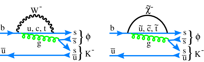
Figure 59: The Standard Model (left) and MSSM (right) contributions to $B^{-}\to\phi K^{-}$.

The $\phi K$ and $\phi K^{*}$ final states have been observed, first by CLEO (Briere 2001) and subsequently by BABAR (Aubert 2001). The BABAR data is shown in Figure 60. The average branching ratio is ${\cal B}(B^{-}\to\phi K^{-})=(6.8\pm 1.3)\times 10^{-6}$ showing that in principle large samples can be acquired especially at hadronic machines.

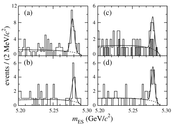
Figure 60: Projections of the maximum likelihood fit onto the $B$ candidate mass $m_{ES}$ from BABAR. (a) $B^{+}\to\phi K^{+}$; (b) $B^{o}\to\phi K^{o}$; (c) $B^{+}\to\phi K^{*+}$; (d) $B^{o}\to\phi K^{*o}$. In (c) the histogram is the sum of the two contributing $K^{*}$ channels while the shaded area is $K^{o}\pi^{+}$ alone (the other channel is $K^{+}\pi^{o}$). The solid line shows the projection of the signal plus background fit while the dashed line shows the projection of the background only.

8.3.2 Other New Physics Models

There are many other specific models that predict New Physics in $b$ decays. I list here a few of these with a woefully incomplete list of references, to give a flavor of what these models predict.

• Two Higgs and Multi-Higgs Doublet Models- They predict large effects in $\epsilon_{K}$ and CP violation in $D^{o}\to K^{-}\pi^{+}$ with only a few percent effect in $B^{o}$ (Nir 1999). Expect to see 1-10% CP violating effects in $b\to s\gamma$ (Wolfenstein 1994).

• Left-Right Symmetric Model- Contributions compete with or even dominate over Standard Model contributions to $B_{d}$ and $B_{s}$ mxing. This means that CP asymmetries into CP eigenstates could be substantially different from the Standard Model prediction (Nir 1999).

• Extra Down Singlet Quarks- Dramatic deviations from Standard Model predictions for CP asymmetries in $b$ decays are not unlikely (Nir 1999).

• FCNC Couplings of the $Z$ boson- Both the sign and magnitude of the decay leptons in $B\to K^{*}\ell^{+}\ell^{-}$ carry sensitive information on new physics. Potential effects are on the of 10% compared to an entirely negligable Standard Model asymmetry of $\sim 10^{-3}$ (Buchalla 2000). These models also predict a factor of 20 enhancement of $b\to d\ell^{+}\ell^{-}$ and could explain a low value of $\sin 2\beta$ (Barenboim 2001a).

• Noncommutative Geometry- If the geometry of space time is noncommutative, i.e. $[x_{\mu},x_{\nu}]=i\theta_{\mu\nu}$, then CP violating effects may be manifest a low energy. For a scale $<$2 TeV there are comparable effects to the Standard Model (Hinchliffe 2001b).

• MSSM without new flavor structure- Can lead to CP violation in $b\to s\gamma$ of up to 5% (Bartl 2001). Ali and London propose (Ali 1999) that the Standard Model formulas are modified by Supersymmetry as

  $$\Delta m_{d} = \Delta m_{d}{\rm(SM)}\left[1+f\left(m_{\chi^{\pm}_{2}},m_{\tilde{t}_{R}},m_{H^{\pm}},tan\beta\right)\right]$$ (121)

  $$\Delta m_{s} = \Delta m_{s}{\rm(SM)}\left[1+f\left(m_{\chi^{\pm}_{2}},m_{\tilde{t}_{R}},m_{H^{\pm}},tan\beta\right)\right]$$ (122)

  $$\left|\epsilon_{K}\right| = {G_{F}^{2}f^{2}_{K}M_{K}M_{W}^{2}\over 6\sqrt{2}\pi^{2}\Delta M_{K}}B_{K}(A^{2}\lambda^{6}\overline{\eta})\left[y_{c}\left(\eta_{ct}f_{3}(y_{c},y_{t})-\eta_{cc}\right)\right.$$ (123)

  $$\left.+\eta_{tt}y_{t}f_{s}(y_{t})\left[1+f\left(m_{\chi^{\pm}_{2}},m_{\tilde{t}_{R}},m_{H^{\pm}},tan\beta\right)\right]A^{2}\lambda^{4}(1-\overline{\rho})\right]~{}~{},$$

  where $\Delta m(SM)$ refers to the Standard Model formula and the expression for $\left|\epsilon_{K}\right|$ would be the Standard Model expression if $f$ were set equal to zero. Ali and London show that it is reasonable to expect that $0.8>f>0.2$ so since the CP violating angles will not change from the Standard Model, determining the value of $(\rho,~{}\eta)$ using the magnitudes $\Delta m_{s}/\Delta m_{d}$ and $|\epsilon_{K}|$ will show an inconsistency with values obtained using other magnitudes and angles.

• Extra Dimensions- We are beginning to see papers predicting $b$ decay phenomena when the world has extra dimensions. See (Agashe 2001) (Barenboim 2001b) (Branco 2001) (Chang 2001) and (Papavassiliou 2000).

I close this section with a quote from Masiero and Vives (Masiero 2001): “The relevance of SUSY searches in rare processes is not confined to the usually quoted possibility that indirect searches can arrive ‘first’ in signaling the presence of SUSY. Even after the possible direct observation of SUSY particles, the importance of FCNC and CP violation in testing SUSY remains of utmost relevance. They are and will be complementary to the Tevatron and LHC establishing low energy supersymmetry as the response to the electroweak breaking puzzle.”

I agree, except that I would replace “SUSY” with “New Physics.”

8.4 Expected Data Samples

It is clear that precision studies of $b$ decays can bring a wealth of information to bear on new physics, that probably will be crucial in sorting out anything seen at the LHC. This is possible because we do expect to have data samples large enough to test these ideas from existing and approved experiments. In Table 13 I show the expected rates in BTeV for one year of running ($10^{7}$ s) and an $e^{+}e^{-}$ $B$-factory operating at the $\Upsilon(4S)$ with a total accumulated sample of 500 fb${-1}$, about what is expected around 2006. (LHCb numbers are the same order of magnitude as the BTeV numbers for many of the modes.)

Table 13: Comparisons of BTeV and $B$-factory Yields on Different Time Scales.

Mode	BTeV $(10^{7})s$			$B$-factory (500 fb-1)
	Yield	Tagged†	S/B	Yield	Tagged†	S/B
$B_{s}\to J/\psi\eta^{(^{\prime})}$	22000	2200	$>$15
$B^{-}\to\phi K^{-}$	11000	11000	$>$10	700	700	4
$B^{o}\to\phi K_{s}$	2000	200	5.2	250	75	4
$B^{o}\to K^{*o}\mu^{+}\mu^{-}$	4400	4400	11	$\sim$50	$\sim$50	?
$D^{*+}\to\pi^{+}D^{o}$; $D^{o}\to K^{-}\pi^{+}$	$\sim 10^{8}$	$\sim 10^{8}$	large	$8\times 10^{5}$	$8\times 10^{5}$	large
$\dagger$ Tagged here means that the intial flavor of the $B$ is determined.

9 Conclusions

I have attempted to cover the length and breadth of $b$ physics, and have only scratched the surface. There is much more to be said and much more to learn. Why are there three families? What is the connection with neutrinos and that mixing matrix? How do we explain the mystery of flavor? These and many more unanswered questions I leave to the students.

Acknowledgments

This research was supported by the US National Science Foundation. I thank Ken Peach and Steve Playfer for a well organized and interesting school that was very enjoyable to attend. The sunny day at the Himalayas was memorable.

I thank Jon Rosner for several seminal discussions during the course of the school. My colleagues at BTeV and CLEO contributed much to my understanding. In particular I thank, M. Artuso, J. Butler and T. Skwarnicki.

References

Abe F, et al., 1998, Phys. Rev. D 58, p.5513, [hep-ex/9804012].

Abe K, et al., 2001a, Measurement of Branching Fractions for $B\to\pi\pi$, $K\pi$ and $KK$ Decays, Phys. Rev. Lett. 87, p.101801, [hep-ex/0104030].

Abbiendi G, et al., 2000, Phys. Lett. B 482, p.15 [hep-ex/0003013].

Abreu P, et al., 2000, Determination of $|V_{ub}|/|V_{cb}|$ with DELPHI at LEP, Phys. Lett. B 478, p.14 [hep-ex/0105054].

Abreu P, et al., 2001, Phys. Lett. B 510, p.55 [hep-ex/0104026].

Acciarri M, et al., 1998, Phys. Lett. B 436, p.174.

Agashe K, Deshphande NG and Wu GH, 2001, Universal Extra Dimensions and $b\to s\gamma$, Phys. Lett. B 514, p.309 [hep-ph/0105084].

Ahmed S, et al., 2000, Phys. Rev. D,62, p.112003 [hep-ex/0008015].

Akers R, et al., 1995, Z. Phys. C 66, p.555.

Alam MS, et al., 1995, Phys. Rev. Lett., 74, p.2285.

Albajar, et al., 1987, Phys. Lett. B 186, p.247, erratum-ibid B197 p.565.

Albrecht H, et al., 1983, Phys. Lett. B 192, p.245.

Albrecht H, et al., 1990, Phys. Lett. B 234, p.16.

Aleksan R, Dunietz I and Kayser B, 1992, Z. Phys. C 54, p.653.

Aleksan R, Kayser B and London D, 1994, Phys. Rev. Lett. 73, p.18 [hep-ph/9403341].

Aleksan R, et al., 1995, Z. Phys. C 67, p.251 [hep-ph/9407406.

Alexander J, et al., 1996, Phys. Rev. Lett. 77, p.5000.

Alexander J, et al., 2001, Phys. Rev. D 64, p.092001 [hep-ex/0103021].

Ali A and Greub C, 1991 , Phys. Lett. B 259, p.182.

Ali A, Kramer G and Lu CD, 1999, Phys. Rev. D 59 p.014005 [hep-ph/9805403].

Altarelli G, 1982, Nucl. Phys. B, 208, p.365.

Ammar R, et al., 1993, Phys. Rev. Lett., 71, p.674.

Appel JA, et al., 2001, Performance of Prototype BTeV Silicon Pixel Detectors in a High Energy Pion Beam, [hep-ex/0108014].

Artuso M, 1994, Experimental Facilities for b-quark Physics, in $B$ Decays 2nd Edition ed. S. Stone, World Scientific, Singapore, p.80.

Artuso M and Barberio E, 2001, Private communication; also see
http://www-cdf.lbl.gov/$\sim$weiming/vcb_summary_ckm_workshop.ps .

Atwood D, Dunietz I and Soni A, 1997, Phys. Rev. Lett. 78, p.3257.

Atwood M and Jaros RA, 1994, Lifetimes, $B$ Decays 2nd Edition ed. S. Stone, World Scientific, Singapore, p. 364.

Aubert B, et al., 2001, Phys. Rev. Lett., 87, p.151801, [hep-ex/0105001].

Ball P and Braun VM, 1998, Phys. Rev. D 58, p.094016.

Bander M, Silverman D and Soni A, 1979, Phys. Rev. Lett., 43, p.242.

Barate R, et al., 1998, Phys. Lett. B 429, p.169.

Barate R, et al., 1999, Eur. Phys. J. C6, p.555.

Barenboim G, Botella FJ and Vives O, 2001a, Phys. Rev. D 64, p.015007 [hep-ph/0012197].

Barenboim G, Botella FJ and Vives O, 2001b, Constraining Models With Vector-Like Fermions from FCNC in K and B Physics, Nucl. Phys. B 613, p.285 [hep-ph/01050306].

Bartl A, et al., 2001, Phys. Rev. D 64, p.076009 [hep-ph/0103324].

Bauer CW, Pirjol D and Steward IW, 2001, A Proof of Factorization for $B\to D\pi$, UCSD-01-12 [hep-ph/0107002].

Bauer M and Wirbel M, 1989, Z. Phys. C 42, p.671.

Bauer CW, Ligeti Z and Luke M, 2001, Precision Determination of $|V_{ub}|$ ¿From Inclusive Decays, UTPT-01-08 [hep-ph/0107074].

Beneke M, et al., 2000, Nucl Phys. B 591, p.313 [hep-ph/0006124].

Beneke M, et al., 2001, Nucl Phys. B 606, p.245 [hep-ph/0104110].

Beyer M and Melikhov D, 1998, Phys. Lett. B 436, p.344 [hep-ph/9807223].

Bigi II, et al., 1997, Annu. Rev. Nucl. Part. Sci. 47, p.591.

Bigi II and Sanda AI, 2000, CP Violation, Cambridge University Press, Cambridge, UK.

Bona M, 2001, BABAR-CONF-01/71, SLAC-PUB-9045 [hep-ex/0111017].

Bortoletto D and Stone S, 1990, Phys. Rev. Lett. 65, p.2951.

Branco GC, de Gouvea A and Rebelo MN, 2001, Split Fermions in Extra Dimensions and CP Violation, Phys. Lett. B 506, p.115 [hep-ph/0012289].

Briere RA, et al., 2001, Phys. Rev. Lett. 86, p.3718, [hep-ex/0101032].

Browder TE, Honscheid K and Pedrini D, 1996, Nonleptonic Decays and Lifetimes of b-quark and c-quark Hadrons, Ann. Rev. Nucl. Part. Sci. 46, p.395 [hep-ph/9606354].

BTeV C, 2000, BTeV An Experiment to Measure Mixing, CP Violation and Rare Decays of Beauty and Charm at the Fermilab Collider, [hep-ex/0006037].

Buchalla G, Hiller G and Isidori G, 2000, Phys. Rev. D 63, p.014015 [hep-ph/0006136].

Buras AJ, 1995, Nucl. Instrm. and Meth. A, 368, p.1.

Buskulic D, et al., 1997, Phys. Lett. B 395, p.373.

Caprini I, Lellouch L and Neubert M. Nucl. Phys. B 530, p.153 [hep-ph/9712417].

Chang D, Keung WY and Mohapatra RN, 2001, Models for Geometric CP Violation With Extra Dimensions, Phys. Lett. B 515, p.431 [hep-ph/0105177].

Chen S, 2001, Branching Fraction and Photon Energy Spectrum for $b\to s\gamma$, [hep-ex/0108032].

Ciuchini M, 2001, JHEP 0107, p.23 [hep-ph/0012308].

Clegg AB and Donnachie A, 1994 Z. Phys. C 62, p.455.

Debbio LD et al., 1998, Phys. Lett. B 416, p.392.

Desphande NG, 1994, Theory of Penguins in $B$ Decays, in $B$ Decays 2nd Edition ed. S. Stone, World Scientific, Singapore, p. 80 and references therein.

Dighe A, Dunietz I and Fleischer R, 1998, Phys. Lett. B 433, p.147 [hep-ph/9804254].

Du D-S, Dunietz I and Wu D-D, 1986, Phys. Rev. D 34, p.3414.

Ellis J, 2000, Highlights of CP 2000, Nucl. Phys. Proc. Suppl. 99A, p.331 [hep-ph/0011396].

Fleischer R and Mannel T, 1998, Phys. Rev. D 57, p.2752 [hep-ph/9704423].

Fleischer R and Buras AJ, 2000, Constraints on $\gamma$ and Strong Phases from $B\to\pi K$ Decays,” presented at ICHEP 2000, Osaka, Japan, July 2000. To appear in the Proceedings [hep-ph/0008298].

Fulton R, et al., 1990, Phys. Rev. Lett., 64, p.16.

Gaillard M and Lee B, 1974, Phys. Rev. D 10, p.897.

Gao Y and Würthwein F, 1999, [hep-ex/9904008].

Gavela MB, Hernández P, Orloff J and Pène O, 1993, Standard Model CP Violation and Baryon Asymmetry, Mod. Phys. Lett. A 9, p.795 [hep-ph/9312215].

Gilman FJ and Singleton R, 1990, Phys. Rev. D 41, p.142.

Greub FJ, Ioannissian A and Wyler D, 1995, Phys. Lett. B 346, p.149 [hep-ph/9408382].

Grinstein B, Isgur N and Wise MB, 1986 Phys. Rev. Lett. 56, p.258.

Gronau M and Wyler D, 1991, Phys. Lett. B 265, p.172.

Groom DE, et al., 2001, The Particle Data Group, The European Physics Journal C 15, p.1.

Grossman Y and Quinn HR, 1997, Phys. Rev. D 56 p.7259 [hep-ph/9705356].

Hashimoto S, et al., 2001, “Lattice Calculation of the Zero-recoil Form Factor of $\overline{B}\to D^{*}\ell^{-}\bar{\nu}$: Toward a Model Independent Determination of $|V_{cb}|$,” [hep-ph/0110253].

Heltsley BK, 2001, CKM Status and Prospects, To appear in Proceedings of XXI Physics in Collision, Seoul, Korea, June, 2001, [hep-ph/0110260]/

Hinchliff I and Kersting N, 2001a, Constraining CP Violating Phases of the MSSM, Phys. Rev. D 63, p.015003 [hep-ph/0003090].

Hinchliff I and Kersting N, 2001b, CP Violation from Noncommutative Geometry, LBNL-47750 [hep-ph/0104137].

Hocker A, Lacker H, Laplace S, Le Diberder F, 2001, A New Approach to a Global Fit of the CKM Matrik, Eur. Phys. J. C 21, p.25 [hep-ph/0104062].

Hurth T, 2001, “Inclusive Rare B Decays, CERN-TH/2001-146, [hep-ph/0106050].

Isgur N and Scora D, Grinstein B and Wise MB, 1989, Phys. Rev. D 39, p.799.

Isgur N and Wise MB, 1990, Phys. Lett. B 237, p.527.

Isgur N and Wise MB, 1994, “Heavy Quark Symmetry,” in $B$ Decays 2nd Edition ed. S. Stone, World Scientific, Singapore, p. 231 and references therein.

Isgur N and Scora D, 1995, Phys. Rev. D 52, p.2783.

Isgur N, 1999, Duality-Violating $1/m_{Q}$ Effects in Heavy Quark Decays, Phys. Lett. B, 448, p.111 [hep-ph/98113777].

Kayser B, 1997, Cascade Mixing and the CP-Violating Angle Beta, [hep-ph/9709382],

Kobayashi M and Maskawa K, 1973, Prog. Theor. Phys. 49, p.652.

Körner JG and Schuler GA, 1988, Z. Phys. C 38, p.511.

Leroy O, 2001, http://lepbosc.web.cern.ch/LEPBOSC/people.html and references therein.

Ligeti Z and Wise M, 1996, Phys. Rev. D 53, p.4937.

Lingel K, Skwarnicki T and Smith JG, 1998, Penguin Decays of B Mesons, Ann. Rev. of Nucl. & Part. Science 48, p.253 [hep-ex/9804015].

Luke M, 1990, Phys. Lett. B 252 p.447.

Masiero A and Vives O, 2000, New Physics Behind the Standard Model’s Door?, Int. School on Subnuclear Physics, Erice, Italy, 1999 [hep-ph/0003133].

Masiero A and Vives O, 2001, New Physics in CP Violation Experiments, Ann. Rev. of Nucl. & Part. Science 51, [hep-ph/0104027].

Mele S, 1999, Phys. Rev. D 59, p.113011.

Melikhov D, 1996, Phys. Rev. D 53, p.2460.

Muheim F, 2001, Status of the LHCb Experiment, Nucl. Instrum and Meth. A 462, p. 233 [hep-ex/0012059].

Neubert M, 1991, Phys. Lett. B 264, p.455.

Neubert M, 1996, Int. J. Mod. Phys. A 11, p.4173 [hep-ph/9604412].

Neubert M and Stech B, 1997, “Non-Leptonic Weak Decays of B Mesons, in Heavy Flavours, 2nd Edition, ed. Buras AJ and Lindner M, World, Scientific, Singapore, p.294 [hep-ph/9705292].

Neubert M and Rosner JL, 1998, Phys. Rev. Lett. 81, p.5076 [hep-ph/9809311].

Neubert M, 2000, JHEP 7, p.22 [hep-ph/0006068].

Nir Y, 1999, CP Violation In and Beyond the Standard Model, IASSNS-HEP-99-96 [hep-ph/9911321].

Papavassiliou J and Santamaria A, 2001, Extra Dimensions at the One Loop Level: $Z\to b\overline{b}$ and $B-\overline{B}$ Mixing, Phys. Rev. D 63, p.016002 [hep-ph/016002].

Peskin ME, 2000, Theoretical Summary Lecture for EPS HEP99, to appear in proceedings [hep-ph/0002041].

Ramirez C, Donoghue JF, and Burdman G, 1990, Phys. Rev. D 41, p.1496.

Richman JD and Burchat PR, 1995, Rev. Mod. Phys. 67, p.893 and references therein.

Rosner J, 2001, The Standard Model in 2001, In these proceedings, and references therein [hep-ph/0108195].

Sachrajda CT, 1999, Lattice B-physics, Nucl. Instru. and Meth. A 462, p.23 [hep-lat/9911016].

Sharma VA and Weber FV, 1994, Recent Measurements of the Lifetimes of b Hadrons, $B$ Decays 2nd Edition ed. S. Stone, World Scientific, Singapore, p. 395.

Silva JP and Wolfenstein L, 1997, Phys. Rev. D 55, p.5331 [hep-ph/9610208].

Skwarnicki T, 2001, Overview of the BTeV Experiment, Nucl. Instrum and Meth. A 462, p. 227.

Snyder AE and Quinn HR, 1993, Phys. Rev. D 48, p.2139.

Stone S, 2000, Hadronic $B$ Decays to Charm from CLEO, in Proc. of XXXth Int. Conf. on High Energy Physics, Aug. 2000, Osaka, Japan p.842 [hep-ex/0008070].

Tajima H, 2001, “Belle B Physics Results,” To appear in Proceedings of the XX Int. Symp on Lepton and Photon Interactions at High Energies, July, 2001, Rome, Italy, [hep-ex/0111037].

Wirbel M, et al., 1985, Z. Phys. C 25, p.627.

Wirbel M, Stech B and Bauer M, 1989, Z. Phys. C 29, p.637.

Wise M, 2001, “Recent Progress in Heavy Quark Physics,” To appear in Proceedings of the XX Int. Symp on Lepton and Photon Interactions at High Energies, July, 2001, Rome, Italy, [hep-ph/0111167].

Wolfenstein L, 1983, Phys. Rev. Lett. 51, p.1945.

Wolfenstein L and Wu YL, 1994, Phys. Rev. Lett. 74, p.2809 [hep-ph/9410253].