A detailed next-to-leading order QCD analysis of deeply virtual Compton scattering observables

Abstract

We present a detailed next-to-leading order (NLO) leading twist QCD analysis of deeply virtual Compton scattering (DVCS) observables, for several different input scenarios, in the $\overline{\mbox{MS}}$ scheme. We discuss the size of the NLO effects and the behavior of the observables in skewedness $\zeta$, momentum transfer, $t$, and photon virtuality, $q^{2}=-Q^{2}$. We present results on the amplitude level for unpolarized and longitudinally polarized lepton probes, and unpolarized and longitudinally polarized proton targets. We make predictions for various asymmetries and for the DVCS cross section and compare with the available data.

I Introduction

In the quest for understanding the structure of hadrons, hard, exclusive lepton-nucleon processes have emerged as very promising candidates to further constrain the dynamical degrees of freedom of hadronic matter. Experimentally, such processes are typified by a clear spatial separation of the scattered final state nucleon and the diffractively-produced, exclusive system, $X$, i.e. by the presence of a large rapidity gap. The hard scale required for a perturbative analysis is either provided by the spacelike virtuality, $Q^{2}=-q^{2}\gg\Lambda^{2}_{\mbox{{QCD}}}$, of the exchanged photon, a heavy quark mass, or by a large momentum transfer to the hadron in the t-channel, $t\ll 0$. Deeply virtual Compton scattering (DVCS) [1, 2, 3, 4, 5, 6, 7, 8, 9, 10, 11, 12, 13], $\gamma^{*}(q)+p(P)\to\gamma(q^{\prime})+p(P^{\prime})$, is the most promising of these processes. One reason for this is that on the lepton level it interferes with a competing QED process, known as the Bethe-Heitler (BH) process, in which the final state photon is radiated from either the initial or final state lepton. The associated interference term offers the unique possibility to directly measure both the imaginary and real parts of QCD amplitudes, via various angular asymmetries. A factorization theorem has been proven for the DVCS process [6, 7] which relates the experimentally-accessible amplitudes to a new class of fundamental functions, called generalized parton distributions (GPDs) [1, 2, 3, 15, 16, 17], which encode detailed information about the partonic structure of hadrons.

GPDs are an extension of the well-known parton distribution functions (PDFs) appearing in inclusive processes such as deep inelastic scattering (DIS), or Drell-Yan, and encode additional information about the partonic structure of hadrons, above and beyond that of conventional PDFs. They are defined as the Fourier transforms of non-local light-cone operators sandwiched between nucleon states of different momenta, commensurate with a finite momentum transfer in the t-channel to the final state proton. As such, the GPDs depend on four variables ($X,\zeta,Q^{2},t$) rather than just two ($X,Q^{2}$) as is the case for regular PDFs. This allows an extended mapping of the dynamical behavior of a nucleon in the two extra variables, skewedness $\zeta$, and momentum transfer, $t$. In fact, knowledge of the behavior of the GPDs in these two extra variables would allow one to obtain, for the first time, a three dimensional map of the proton in terms of its partonic constituents. The GPDs are true two-particle correlation functions, whereas the PDFs are effectively only one-particle distributions. They contain, in addition to the usual PDF-type information residing in the so-called “DGLAP region” [18] (for which the momentum fraction variable is larger than the skewedness parameter, $X>\zeta$), supplementary information about the distribution amplitudes of virtual “meson-like” states in the nucleon in the so-called “ERBL region” [19] ($X<\zeta$).

A good knowledge of GPDs is required to establish the boundary conditions for a large class of exclusive processes calculable in QCD. Unfortunately, reliable perturbative calculations can only be made if $t$ is either small or large, confining a sensible comparison between theory and experiment to restricted kinematical regions where either the $t$-dependence is a purely nonperturbative function (small $t$, large $Q^{2}$) as in DVCS or the $Q^{2}$-dependence is mainly non perturbative (small $Q^{2}$, large $t$) as in, for example, large-$t$ photoproduction of a real photon (wide angle DVCS) [20]. In light of this observation, one might question the practicality of studying and measuring these exclusive distributions, given that inclusive PDFs may only be constrained well via a global analysis of a large number of data points from numerous experiments.

It turns out that the GPDs are rather more tightly constrained than one might naively assume [21]. Firstly, they are obliged to reproduce the regular PDFs in the forward limit $\zeta\to 0$ [1, 2, 3]. Secondly, they are each required to be either symmetric or antisymmetric about the point $X=\zeta/2$ in the ERBL region, and they have to obey a polynomiality constraint (see for example [22]). These are properties which need to be preserved under evolution. Lastly, the DVCS amplitudes, and thus certain observables, seem to be very sensitive to the shape of the GPD in the small $\zeta$ region, especially the real part of DVCS amplitudes [23, 24]. Hence, experimental measurements of DVCS observables, even of only moderate statistics, appear to give a good opportunity to pin-down the GPDs, given these theoretical restrictions. Therefore a careful, thorough and accurate theoretical analysis of DVCS is necessary to understand how varying the input GPDs affects the physical observables and the quantitative and qualitative changes in going from leading order (LO) to next-to-leading order (NLO) accuracy in perturbation theory. In this paper, we present such a NLO analysis, in the $\overline{\mbox{MS}}$-scheme, for both polarized and unpolarized scattering, and explore some of the necessary issues required to make an optimal extraction of the GPDs from current and future data.

The physical picture emerging for DVCS is also very interesting in its own right. Several important questions immediately arise. What does the energy and $Q^{2}$-dependence of DVCS reveal about the nature of diffractive exchange and how does it compare to other diffractive processes ? Why does DVCS appear to have significant probability in the valance region at larger $x$, i.e. outside of the region in which generic diffraction usually occurs ? Is the physical picture for DVCS the same in both regions ? We will attempt a partial answer to these questions in the following.

This paper gives a comprehensive analysis of DVCS observables at NLO accuracy. Complementary information may be found in [21, 23, 24]. To bring our analysis right up to date, we introduce unpolarized input GPDs based on two of the most recent PDF sets, CTEQ5M [25] and MRST99 [26] (in addition to GRV98 [27], and the older MRSA’ [28] used in our earlier publications). This allows us to push our input scale for skewed evolution down to $Q_{0}=1$ GeV. For the purposes of comparison we also present the results for DVCS observables obtained using our earlier input models. Various computer codes used in our analysis our available from the HEPDATA website [29].

This paper is structured as follows. In section II we reiterate the kinematics of DVCS and BH and define the DVCS observables, i.e. various measurable angular asymmetries and cross sections. In section III we describe the various input GPDs and present numerical results for the NLO evolution [15, 30] of the new sets. Section IV discusses how the various DVCS amplitudes are produced via convolution integrals of GPDs with coefficient functions. We present the $Q^{2}$ and $\zeta$-dependence of the unpolarized amplitudes for the new sets graphically. In section V we give our predictions for the DVCS observables in $\zeta$, $Q^{2}$ and $t$, for various polarizations of probe and target, as well as discussing their implications. We compare our results with the currently available data and with other theoretical predictions in section VI. Finally, we briefly conclude in section VII.

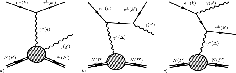
FIG. 1.: a) DVCS graph, b) BH with photon from final state lepton and c) with photon from initial state lepton.

II Kinematics and observables for DVCS and BH

A Kinematics and frame definition

The lepton level process, $e^{\pm}(k,\kappa)~{}N(P,S)\to e^{\pm}(k^{\prime},\kappa^{\prime})~{}N(P^{\prime},S^{\prime})~{}\gamma(q^{\prime},\epsilon^{\prime})$, receives contributions from each of the graphs shown in Fig. 1. The corresponding differential cross section is given by:

$$d\sigma^{DVCS+BH}=\frac{1}{4k\cdot P}|{\cal T}^{\pm}|^{2}(2\pi)^{4}\delta^{(4)}(k+P-k^{\prime}-P^{\prime}-q^{\prime})\frac{d^{3}{\bf k^{\prime}}}{2k^{\prime}_{0}(2\pi)^{3}}\frac{d^{3}{\bf P^{\prime}}}{2P^{\prime}_{0}(2\pi)^{3}}\frac{d^{3}{\bf q^{\prime}}}{2q^{\prime}_{0}(2\pi)^{3}}\,,$$ (1)

where the square of the amplitude receives contributions from pure DVCS (Fig. 1a), from pure BH (Figs. 1b, 1c) and from their interference (with a sign governed by lepton charge),

$$|{\cal T}^{\pm}|^{2}=\sum_{\kappa^{\prime},S^{\prime},\epsilon^{\prime}}\Big{[}|{\cal T}^{\pm}_{DVCS}|^{2}+({\cal T}^{\pm*}_{DVCS}{\cal T}_{BH}+{\cal T}^{\pm}_{DVCS}{\cal T}^{*}_{BH})+|{\cal T}_{BH}|^{2}\Big{]}\,.$$ (2)

The DVCS amplitude is given by

$${\cal T}_{DVCS}^{\pm}=\pm\frac{e^{3}}{q^{2}}\epsilon^{{}^{\prime}\ast}_{\mu}T^{\mu\nu}\bar{u}(k^{\prime})\gamma_{\nu}u(k)\quad\left\{{+\mbox{\ for\ }e^{+}\atop-\mbox{\ for\ }e^{-}}\right.\,,$$ (3)

where $q=k-k^{\prime}$, $\epsilon^{{}^{\prime}*}_{\mu}$ is the polarisation vector of the outgoing real photon, and the hadronic tensor, $T_{\mu\nu}$, is defined by a time ordered product of two electromagnetic currents:

$$T_{\mu\nu}({\bar{q}},P,P^{\prime})=i\int dxe^{ix\cdot{\bar{q}}}\langle P^{\prime},S^{\prime}|Tj_{\mu}(x/2)j_{\nu}(-x/2)|P,S\rangle\,,$$ (4)

where ${\bar{q}}=(q+q^{\prime})/2$. This hadronic tensor contains twelve independent kinematical structures [32] for a spin-1/2 target. Here, we restrict ourselves to the twist-2 part of $T_{\mu\nu}$ and drop all other terms of either kinematical or dynamical higher twist. From the structure of the operator product expansion (OPE) one can immediately conclude that, to twist-2 accuracy, one has the following form factor decomposition:

$$T_{\mu\nu}(q,P,\Delta) = -\tilde{g}_{\mu\nu}\frac{{\bar{q}}\cdot V_{1}}{2{\bar{P}}\cdot{\bar{q}}}-i\tilde{\epsilon}_{\mu\nu\rho\sigma}\frac{{\bar{q}}^{\rho}A_{1}^{\sigma}}{2{\bar{P}}\cdot{\bar{q}}}\,,$$ (5)

where ${\bar{P}}=(P+P^{\prime})/2$ and the gauge invariant tensors $\tilde{g}_{\mu\nu}={\cal P}_{\mu\rho}g_{\rho\sigma}{\cal P}_{\sigma\nu}$ and $\tilde{\epsilon}_{\mu\nu\alpha\beta}={\cal P}_{\mu\rho}\epsilon_{\rho\sigma\alpha\beta}{\cal P}_{\sigma\nu}$ are constructed through the projection tensor ${\cal P}_{\mu\nu}\equiv g_{\mu\nu}-q_{\mu}q^{\prime}_{\nu}/q\cdot q^{\prime}$. The vector $V^{\mu}_{1}$ and axial-vector $A^{\nu}_{1}$ are expressed, again to twist-2 accuracy, through the following form factor decomposition,

$$V_{1\mu}=\bar{U}(P^{\prime},S^{\prime})\left({\cal H}_{1}\gamma_{\mu}-{\cal E}_{1}\frac{i\sigma_{\mu\nu}\Delta^{\nu}}{2M}\right)U(P,S)\,,$$ (6)

$$A_{1\mu}=\bar{U}(P^{\prime},S^{\prime})\left(\widetilde{\cal H}_{1}\gamma_{\mu}\gamma_{5}-\widetilde{\cal E}_{1}\frac{\Delta_{\mu}\gamma_{5}}{2M}\right)U(P,S)\,,$$ (7)

where $U,{\bar{U}}$ are spinors for the incoming and outgoing hadron state, $\Delta=P-P^{\prime}$ is the momentum transfered from the hadron and $M$ is the hadron mass. The various Lorentz structures have associated amplitudes: ${\cal H}_{1},{\cal E}_{1}$ are unpolarized helicity non-flip and helicity flip amplitudes, respectively, and ${\tilde{\cal H}}_{1},{\tilde{\cal E}}_{1}$ are their polarized counterparts. These amplitudes are expressed, via the DVCS factorization theorem [6, 7], as convolutions of a hard scattering coefficient function and a GPD. They depend on the following Lorentz-invariant variables:

$$\xi=\frac{Q^{2}}{2{\bar{P}}\cdot{\bar{q}}}\,,\qquad{\bar{\cal Q}}^{2}=-{\bar{q}}^{2},\qquad t=\Delta^{2}=(P-P^{\prime})^{2}\,,$$ (8)

which are related to the experimentally accessible variables, $\zeta\equiv x_{bj}=-q^{2}/(2P\cdot q)$ and $Q^{2}=-q^{2}$, used throughout this paper, via

$${\bar{\cal Q}}^{2}=\frac{1}{2}Q^{2}\left(1+\frac{t}{Q^{2}}\right)\approx\frac{1}{2}Q^{2},\quad~{}\mbox{and}\quad\xi=\frac{\zeta\left(1+\frac{t}{2Q^{2}}\right)}{2-\zeta\left(1-\frac{t}{Q^{2}}\right)}\approx\frac{\zeta}{2-\zeta}\,.$$ (9)

The BH amplitude is purely real and is given by the sum of the graphs in Fig. 1b and Fig. 1c:

$${\cal T}_{BH}=-\frac{e^{3}}{t}\epsilon^{{}^{\prime}*}_{\mu}L^{\mu\nu}J_{\nu}\,,$$ (10)

with the leptonic tensor

$$L_{\mu\nu}={\bar{u}}(k^{\prime},\kappa^{\prime})\left[\gamma_{\mu}({\not\!k}+{\not\!\Delta})^{-1}\gamma_{\nu}+\gamma_{\nu}({\not\!k^{\prime}}-{\not\!\Delta})^{-1}\gamma_{\mu}\right]u(k,\kappa)\,,$$ (11)

and the hadronic current

$$J_{\nu}={\bar{U}}(P^{\prime},S^{\prime})\left(F_{1}(t)\gamma_{\nu}-iF_{2}(t)\sigma_{\nu\tau}\frac{\Delta^{\tau}}{2M}\right)U(P,S)\,,$$ (12)

where $F_{1},F_{2}$ are the Dirac and Pauli form factors, respectively, normalized such that $F^{p}_{1}(0)=1$, $F^{p}_{2}(0)\equiv\kappa_{p}=-1.79$, and $F^{n}_{1}(0)=0$, $F^{n}_{2}(0)\equiv\kappa_{n}=-1.91$ for proton, $p$, and neutron, $n$. These are known from low energy exclusive scattering and have been parametrised, using dipole formulas for small $t$, as linear combinations of the electric and magnetic form factors:

$$F^{i}_{1}=\frac{G^{i}_{E}(t)+\frac{t}{4M^{2}}G^{i}_{M}(t)}{1+\frac{t}{4M^{2}}},~{}\quad~{}F^{i}_{2}(t)=\frac{G^{i}_{M}(t)-G^{i}_{E}(t)}{1+\frac{t}{4M^{2}}}\,,$$ (13)

with

$$G^{p}_{E}(t)=\frac{G^{p}_{M}(t)}{1+\kappa_{p}}=\frac{G^{n}_{M}(t)}{\kappa_{n}}=\frac{1}{\left(1-\frac{t}{m^{2}_{V}}\right)^{2}},~{}G^{n}_{E}(t)=0\,,$$ (14)

and $m_{V}=0.84~{}\mbox{GeV}$ [33].

Following [34], we chose to work in the $\gamma^{*}P$ frame with the proton at rest such that the direction of the four vector $q=k-k^{\prime}$ (i.e. the virtual photon direction for the DVCS graph) defines the negative $z$-axis . Without loss of generality we can choose the incoming electron to only have a non-zero component along the positive $x$-axis in the transverse ($x-y$) plane: $k=(k_{0},k_{0}\sin\theta_{e},0,k_{0}\cos\theta_{e})$, $q=(q_{0},0,-|q_{3}|)$, $P=(M,0,0,0)$ and $P^{\prime}=(P^{\prime}_{0},|\mbox{\boldmath$P^{\prime}$}|\cos\phi\sin\theta_{H},|\mbox{\boldmath$P^{\prime}$}|\sin\phi\sin\theta_{H},|\mbox{\boldmath$P^{\prime}$}|\cos\theta_{H})$, where $\phi$ is the azimuthal angle between the lepton ($x-z$) and hadron scattering planes. A dependence on the angle $\phi$ can be either induced kinematically, or through the phase of hadronic amplitudes as will be shown below. The spin vectors of the nucleon target for longitudinal and transverse polarizations are given by

$$S^{\pm}_{L}=\frac{\Lambda}{Q\sqrt{1+\frac{Q^{2}}{4M^{2}\zeta^{2}}}}\left(q_{0}-\frac{Q^{2}}{2M\zeta},0,0,-|q_{3}|)\right)\quad,\quad~{}S^{T}=(0,\cos\Phi,\sin\Phi,0)\,,$$ (15)

where $\Lambda=\pm 1$. Note that $t=(P-P^{\prime})^{2}$ has a kinematical minimum value which is given by

$$t_{\mbox{min}}=-\frac{M^{2}x_{bj}^{2}}{1-x_{bj}+\frac{x_{bj}M^{2}}{Q^{2}}}(1+{\cal O}(\frac{M^{2}}{Q^{2}}))\,.$$ (16)

The motivation for using this frame is that the frame-dependent expressions for the $s$- and $u$-channel BH propagators appearing in eq.(11) (cf. Figs. 1b, 1c, respectively) have a particularly simple Fourier expansion in the angle $\phi$. The dimensionless forms ${\cal P}_{1}=\frac{(k+\Delta)^{2}}{Q^{2}}=\frac{t+2k\cdot\Delta}{Q^{2}}$ and ${\cal P}_{2}=\frac{(k-q^{\prime})^{2}}{Q^{2}}=1-\frac{2k\cdot\Delta}{Q^{2}}$ are (up to corrections of order ${\cal O}((-t/Q^{2}),(M^{2}/Q^{2}))$):

$${\cal P}_{1}=\frac{1}{y}\Big{\{}1+2\sqrt{\frac{(t_{\mbox{min}}-t)(1-x)(1-y)}{Q^{2}}}\cos\phi-\frac{t}{Q^{2}}(1-y-x(2-y))-2\frac{M^{2}x^{2}}{Q^{2}}(2-y)\Big{\}}\,,$$ (17)

$${\cal P}_{2}=-\frac{1}{y}\Big{\{}(1-y)+2\sqrt{\frac{(t_{\mbox{min}}-t)(1-x)(1-y)}{Q^{2}}}\cos\phi-\frac{t}{Q^{2}}(1-x(2-y))-2\frac{M^{2}x^{2}}{Q^{2}}(2-y)\Big{\}}\,.$$ (18)

The product ${\cal P}_{1}{\cal P}_{2}$ appears in the BH and interference expressions and thus induces an additional kinematical (rather than hadronic) $\phi$-dependence. In certain kinematical regions, this additional $\phi$-dependence can fake certain hadronic $\phi$-dependences [34], it can also lead to unwanted contributions in certain $\phi$-asymmetries, as discussed below. One way out of this dilemma is to weight DVCS observables with ${\cal P}_{1}{\cal P}_{2}$, leaving only the pure hadronic $\phi$-dependence (exploiting the orthogonality of $\cos\phi$ and $\cos m^{\prime}\phi$ for integer $m^{\prime}\neq 1$). We will not do this here because such a weighting requires a good $\phi$ resolution not available for the present data and also because the pure twist-2 contributions may well explain most of the observed data without needing to take twist-3 or higher contributions into account. Nevertheless, studying weighted DVCS observables should be done as soon as good experimental $\phi$-resolution is available.

B DVCS observables: differential cross section and asymmetries

After performing the phase space integration in eq.(1), the triple differential cross section on the lepton level is given by

$$\frac{d\sigma^{(3)}(e^{\pm}p\to e^{\pm}\gamma p)}{dx_{bj}dQ^{2}d|t|}=\int^{2\pi}_{0}d\phi\frac{d\sigma^{(4)}}{dx_{bj}dQ^{2}d|t|d\phi}\,=\frac{\alpha_{e.m.}^{3}x_{bj}y^{2}}{8\pi Q^{4}}\left(1+\frac{4M^{2}x_{bj}^{2}}{Q^{2}}\right)^{-1/2}\int^{2\pi}_{0}d\phi|{\cal T}^{\pm}|^{2}\,.$$ (19)

The twist two expressions for the DVCS squared, interference and BH squared terms, for all probe and target polarizations, required for eq.(19) are very similar to eqs.(24-32) of [31] but with the full expressions for the BH propagators of eq.(18) included to reinstate the correct $y$- and $\phi$-dependence (a correction factor of $-(1-y)/(y^{2}{\cal P}_{1}{\cal P}_{2})$ should be applied to eqs.(27-32) of [31]).

From the pure DVCS piece (following the usual single photon exchange flux factor convention adopted in [35]), changing variable from $x_{bj}$ to $y$ and integrating over $t$, one may define the virtual-photon proton cross section via

$$\frac{d\sigma^{(2)}(e^{\pm}p\to e^{\pm}\gamma p)}{dydQ^{2}}=\frac{\alpha_{e.m.}(1+(1-y)^{2})}{2\pi Q^{2}y}\sigma(\gamma^{*}P\to\gamma P)\,.$$ (20)

We give predictions for $\sigma(\gamma^{*}P\to\gamma P)$ and compare with the recent experimental data from the H1 Collab. [10] in section VI.

We will now define various DVCS observables, in terms of a list of asymmetries in the azimuthal angle $\phi$:

• The (unpolarized) azimuthal angle asymmetry (AAA), measured in the scattering of an unpolarized probe on an unpolarized target, is defined by

  $$\mbox{AAA}=\frac{\Big{.}\int^{\pi/2}_{-\pi/2}d\phi(d\sigma^{DVCS+BH}-d\sigma^{BH})-\Big{.}\int^{3\pi/2}_{\pi/2}d\phi(d\sigma^{DVCS+BH}-d\sigma^{BH})}{\Big{.}\int^{2\pi}_{0}d\phi d\sigma^{DVCS+BH}}\,,$$ (21)

  where $d\sigma^{BH}$ is the pure BH term.

• The single spin asymmetry (SSA), measured in the scattering of a longitudinally polarized probe on an unpolarized target, is defined by

  $$\mbox{SSA}=\frac{\int^{\pi}_{0}d\phi\Delta\sigma^{DVCS+BH}-\int^{2\pi}_{\pi}d\phi\Delta\sigma^{DVCS+BH}}{\int^{2\pi}_{0}d\phi(d\sigma^{DVCS+BH,\uparrow}+d\sigma^{DVCS+BH,\downarrow})}\,,$$ (22)

  where $\Delta\sigma=d\sigma^{\uparrow}-d\sigma^{\downarrow}$ and $\uparrow$ and $\downarrow$ signify that the lepton is polarized along or against its direction, respectively.

• The asymmetry of an unpolarized probe on a longitudinally polarized target (UPLT) is given by:

  $$\mbox{UPLT}=\frac{\int^{\pi}_{0}d\phi\Delta\sigma_{LT}^{DVCS+BH}-\int^{2\pi}_{\pi}d\phi\Delta\sigma_{LT}^{DVCS+BH}}{\int^{2\pi}_{0}d\phi(d\sigma^{DVCS+BH}_{\uparrow}+d\sigma^{DVCS+BH}_{\downarrow})}\,,$$ (23)

  where $\Delta\sigma_{LT}=d\sigma_{\uparrow}-d\sigma_{\downarrow}$ with $\uparrow$ and $\downarrow$ signifying that the target is polarized along or against the $+z$-direction, respectively, corresponding to $\Lambda=\mp 1$ in eq.(15).

• The asymmetry of an unpolarized probe on a transversely polarized target (UPTT) is given by:

  $$\mbox{UPTT}=\frac{\int^{\pi}_{0}d\phi\Delta\sigma_{TT}^{DVCS+BH}-\int^{2\pi}_{\pi}d\phi\Delta\sigma_{TT}^{DVCS+BH}}{\int^{2\pi}_{0}d\phi(d\sigma^{DVCS+BH}_{\to}+d\sigma^{DVCS+BH}_{\leftarrow})}\,,$$ (24)

  where $\Delta\sigma_{TT}=d\sigma_{\to}-d\sigma_{\leftarrow}$ with $\to$ and $\leftarrow$ signify that the target transverse polarization vector, $S^{T}$, points along the $+x$ and $-x$ directions (i.e. $\Phi=0,\pi$), respectively.

• The charge asymmetry (CA) in the scattering of an unpolarized probe on an unpolarized target:

  $$\mbox{CA}=\frac{\Big{.}\int^{\pi/2}_{-\pi/2}d\phi\Delta d^{C}\sigma^{DVCS+BH}-\Big{.}\int^{3\pi/2}_{\pi/2}d\phi\Delta d^{C}\sigma^{DVCS+BH}}{\Big{.}\int^{2\pi}_{0}d\phi(d^{+}\sigma^{DVCS+BH}+d^{-}\sigma^{DVCS+BH})}\,,$$ (25)

  where $\Delta d^{C}\sigma=d^{+}\sigma-d^{-}\sigma$ corresponds to the difference of the scattering with a positron probe and an electron probe.

• The charge asymmetry with a double spin flip of a longitudinally polarized probe on a longitudinally polarized target (CADSFL):

  $$\mbox{CADSFL}=\frac{\Big{.}\int^{\pi/2}_{-\pi/2}d\phi\Delta d^{C}\sigma_{LT}^{DVCS+BH,LP}-\Big{.}\int^{3\pi/2}_{\pi/2}d\phi\Delta d^{C}\sigma_{LT}^{DVCS+BH,LP}}{\Big{.}\int^{2\pi}_{0}d\phi(d^{+}\sigma^{DVCS+BH}_{\uparrow}+d^{-}\sigma^{DVCS+BH}_{\downarrow})}\,,$$ (26)

  where $\Delta d^{C}\sigma_{LT}^{LP}=d^{+}\sigma^{\uparrow}_{\uparrow}-d^{-}\sigma^{\downarrow}_{\downarrow}-\Delta d^{C}\sigma$ with $d^{+}\sigma^{\uparrow}_{\uparrow}$ corresponding to a positron beam polarized along its own direction scattering with a target with its polarization vector having a positive $z$-component, $d^{-}\sigma^{\downarrow}_{\downarrow}$ corresponds to an electron beam polarized against its own direction scattering on target with its polarization vector having a negative $z$-component and with $\Delta d^{C}\sigma$ having the same meaning as for CA.

• The charge asymmetry with a double spin flip of a longitudinally polarized probe on a transversally polarized target (CADSFT):

  $$\mbox{CADSFT}=\frac{\Big{.}\int^{\pi/2}_{-\pi/2}d\phi\Delta d^{C}\sigma_{TT}^{DVCS+BH,LP}-\Big{.}\int^{3\pi/2}_{\pi/2}d\phi\Delta d^{C}\sigma_{TT}^{DVCS+BH,LP}}{\Big{.}\int^{2\pi}_{0}d\phi(d^{+}\sigma^{DVCS+BH}_{\to}+d^{-}\sigma^{DVCS+BH}_{\leftarrow})}\,,$$ (27)

  where $\Delta d^{C}\sigma_{TT}^{LP}=d^{+}\sigma^{\uparrow}_{\to}-d^{-}\sigma^{\downarrow}_{\leftarrow}-\Delta d^{C}\sigma$, with $d^{+}\sigma^{\uparrow}_{\to}$ corresponding to a positron beam polarized along its own direction scattering on a target with a polarization vector pointing in the $+x$ direction, $d^{-}\sigma^{\downarrow}_{\leftarrow}$ corresponds to an electron beam polarized against its own direction scattering on a target with a polarization vector pointing in the $-x$ direction, and $\Delta d^{C}\sigma$ having the same meaning as in CA.

The definitions above make the asymmetries directly proportional to the real part of a combination of DVCS amplitudes, in the case of the AAA, CA, CADSFT and CADSFL, and to the imaginary part of a combination of DVCS amplitudes for SSA, UPTT and UPLT. If one forms the proper combinations from eqs.(24-32) of [31], with the correction factor included, one observes that for small-$x$ DVCS observables the information from transversally polarized targets is redundant to the information from longitudinally polarized targets as far as the information on the real and imaginary part of DVCS amplitudes is concerned. For large $x$, this is, strictly speaking, no longer true! However, higher twist corrections, especially in the normalization of the asymmetries, will make extraction of information on individual amplitudes virtually impossible. For this reason we will focus only on DVCS observables which may be obtained using an unpolarized or longitudinally polarized target. Note that for small $x$ and $t$, these combinations of amplitudes reduce to just the unpolarized (for AAA, CA and SSA) or polarized (for UPLT and CADSFL) helicity non-flip amplitudes [31]. Note also that the definition of the AAA is different from the usual one (see e.g. the first reference of [8]) and is designed to ensure that the numerator contains only the interference term and is thus directly proportional to a DVCS amplitude. This slight change was necessary since, on inspection, it was realised that the pure BH contribution to the numerator does not vanish when the $\phi$ integrations in the numerator of eq.(21) are carried out (due to the correction factor, $\propto 1/{\cal P}_{1}{\cal P}_{2}$, applied to eq.(27) of [31]). Hence the BH contribution needs to be subtracted from the differential cross section in order to have an asymmetry which is directly proportional to the real part of a hadronic DVCS amplitude.

Note that in the following we will always assume a positron probe, except in the case of charge asymmetries where one needs both positron and electron. Thus for the corresponding electron observables the overall sign in the results we will quote below has to be reversed.

At this point, we wish to make a few general comments on the $\phi$-behavior of the lepton level expressions given in eqs.(30-32) of [31] (modified by the propagator factors). Firstly, one can cleanly separate the real and imaginary parts of DVCS amplitudes using their different $\phi$ behavior either by taking moments with respect to a function in $\phi$ (usually either sine or cosine) thereby projecting out the unwanted contributions, or, equivalently, by forming asymmetries in the angle $\phi$, as we did above. Secondly, as was observed in [4, 34], the $\phi$-dependence of the expressions also allows a clean separation into different twist contributions. For example (see [34]), the real and imaginary parts of twist-2 can be separated from one another by using $\phi$-moments, since the real and imaginary parts of twist-3 amplitudes have a $\phi$-dependence which is very different from that of twist-2: e.g. $\cos\phi$ (twist-2) and $\cos 2\phi$ (twist-3) [4, 34]. Thus DVCS allows the real and imaginary parts of hadronic twist-2 and twist-3 amplitudes to be isolated for the first time within the same experiment, simply by using different moments or asymmetries in the azimuthal angle $\phi$. Therefore, experimental upgrades which enhance the instrumentation in the forward region (see e.g. [36] for a H1 Collaboration proposal) are vital to maximise the physics scope of these experiments. We note the asymmetries as defined above do not necessarily require a good resolution in the angle $\phi$, it is sufficient to specify which hemisphere in $\phi$ a given event corresponds to. A reasonable sample of events will then be sufficient to measure the asymmetries. If one wishes to produce asymmetries weighted for example with a sine or cosine, then a good phi resolution is of course required. This concludes our comments on DVCS/BH kinematics and DVCS observables.

III GPDs and input models

A Symmetries and representations of GPDs

For the definition of our input GPDs we follow precisely the prescription given in [21]. GPDs result from matrix elements for quark and gluon correlators of unequal momentum nucleon states and may be defined in a number of ways. Following [2, 3], we initially chose a definition which treated the initial and final state nucleon momentum ($P,P^{\prime}$, respectively) symmetrically by involving parton light-cone fractions with respect to the momentum transfer, $\Delta=P-P^{\prime}$, and the average momentum, $\bar{P}=(P+P^{\prime})/2$. The inherent symmetries of the matrix elements are clearly manifest in associated symmetries of the GPDs. We then shifted to a definition [37] based on light-cone fractions of the incoming hadron, for the purposes of evolution and a direct comparison with conventional PDFs and with experiment. We discussed the manifestation of the symmetries in this representation and explicitly illustrated their preservation under evolution.

Matrix elements of the non-local operators are defined on the light cone and involve a light-like vector $z^{\mu}$ ($z^{2}=0$). They can be most generally represented by a double spectral representation with respect to $\bar{P}\cdot z$ and $\Delta\cdot z$ [1, 2, 22] (see eq.(4) of [21]). In accordance with the associated Lorentz structures, the non-singlet, singlet and gluon matrix elements involve functions corresponding to proton helicity conservation (labelled with $F$) and to proton helicity flip (labelled with $K$) which are collectively known as double distributions. Henceforth, for brevity, we shall only discuss the helicity non-flip parts explicitly. However, the helicity flip case is exactly analogous. The $D$-terms in eq.(4) of [21] correspond to resonance-like exchange[22, 38] and permit non-zero values for the singlet and gluon matrix elements in the limit $\bar{P}\cdot z\to 0$ and $\Delta\cdot z\neq 0$, which is allowed by their evenness in $\bar{P}\cdot z$.

By making a particular choice of the light-cone vector, $z^{\mu}$, as a light-ray vector (so that in light-cone variables, $z_{\pm}=z_{0}\pm z_{3}$, only its minus component is non-zero: $z^{\mu}=(0,z_{-},{\vec{0}})$) one may reduce the double spectral representation of eq.(4) of [21], defined on the entire light-cone, to a one dimensional spectral representation, defined along a light ray, depending on the skewedness parameter, $\xi$, defined by

$$\xi=\Delta\cdot z/2\bar{P}\cdot z=\Delta_{+}/2{\bar{P}}_{+}\,,$$ (28)

which is equivalent to our definition in Sec. II (cf. eq.(9)). The resultant GPDs are the off-forward parton distribution functions (OFPDFs) introduced in [1, 4]:

$$H(v,\xi,t)=\int^{1}_{-1}dx^{\prime}\int^{1-|x^{\prime}|}_{-1+|x^{\prime}|}dy^{\prime}\delta(x^{\prime}+\xi y^{\prime}-v)F(x^{\prime},y^{\prime},t)\,,$$ (29)

where $v\in[-1,1]$. In terms of individual flavor decompositions, the singlet, non-singlet and gluon distributions are given through

$$H^{S}(v,\xi)=\sum_{a}H^{q,a}(v,\xi)\mp H^{q,a}(-v,\xi)\,,$$ (30)

$$H^{NS,a}(v,\xi)=H^{q,a}(v,\xi)\pm H^{q,a}(-v,\xi)\,,$$ (31)

$$H^{G}(v,\xi)=H^{g}(v,\xi)\pm H^{g}(-v,\xi)\,,$$ (32)

where the upper (lower) signs corresponds to the unpolarized (polarized) case. Note that the symmetries which hold for the matrix elements can change for the $H^{i}$s, due to the influence of the $\bar{P}\cdot z$, $\hat{z}$ factors in eq.(4) of [21]. In particular, the unpolarized quark singlet is antisymmetric about $v=0$, as are both $D$-terms, whereas the unpolarized quark non-singlet and the gluon are symmetric. The opposite symmetries hold for the polarized distributions. The helicity flip GPDs, are found analogously (double integrals with respect to the $K$s) and similar reasoning establishes their symmetry properties.

As in [21], we shall make the usual assumption that the $t$-dependence of all of these functions factorizes into implicit form factors. One should bear in mind that in order to make predictions for physical amplitudes (for $t\neq 0$) these form factors must be specified. Note that the assumption of a factorized $t$-dependence, as a general statement, must be justified within the kinematic regime concerned. It appears to be valid at small $x$ and small $t$, from the HERA data on a variety of diffractive measurements. However, it appears not to hold for moderate to large $t$ and larger $x$ [39].

For the purposes of comparing to experiment it is natural to define GPDs in terms of momentum fractions, $X\in[0,1]$, of the incoming proton momentum, $P$, carried by the outgoing parton. To this end we adapt the notation and definitions of [37] introducing two non-diagonal parton distribution functions (NDPDFs), ${\cal F}^{q}$ and ${\cal F}^{\bar{q}}$, for flavor, $a$:

$${\cal F}^{q,a}\left(X_{1}=\frac{v_{1}+\xi}{1+\xi},\zeta\right)=\frac{H^{q,a}(v_{1},\xi)}{(1-\zeta/2)},\qquad{\cal F}^{{\bar{q}},a}\left(X_{2}=\frac{\xi-v_{2}}{1+\xi},\zeta\right)=-\frac{H^{q,a}(v_{2},\xi)}{(1-\zeta/2)}\,,$$ (33)

where $v_{1}\in[-\xi,1],\,v_{2}\in[-1,\xi]$ (see Fig. 4 of [37]), $\zeta\equiv\Delta^{+}/P^{+}$ is the skewedness defined on the domain $\zeta\in[0,1]$ such that $\xi\approx\zeta/(2-\zeta)$ and $\zeta=x_{bj}$ for DVCS (this definition is equivalent and the relations are the same as those in Sec. II). The transformations between the $v_{1},v_{2}$ and $X_{1},X_{2}$ are given implicitly in eq.(33), the inverse transformations are:

$$v_{1}=\frac{X_{1}-\zeta/2}{1-\zeta/2}\,, ~{}v_{2}=\frac{\zeta/2-X_{2}}{1-\zeta/2}\,.$$ (34)

For the gluon one may use either transformation, e.g.

$${\cal F}^{g}(X,\zeta) = \frac{H^{g}(v_{1},\xi)}{(1-\zeta/2)}\,.$$ (35)

There are two distinct kinematic regions for the GPDs, with different physical interpretations. In the DGLAP [18] region, $X>\zeta$ ($|v|>\xi$), ${\cal F}^{q}(X,\zeta)$ and ${\cal F}^{\bar{q}}(X,\zeta)$ are independent functions, corresponding to quark or anti-quark fields leaving the nucleon with momentum fraction $X$ and returning with positive momentum fraction $X-\zeta$. As such they correspond to a generalization of regular DGLAP PDFs (which have equal outgoing and returning fractions). In the ERBL [19] region, $X<\zeta$ ($|v|<\xi$), both quark and anti-quark carry positive momentum fractions ($X,\zeta-X$) away from the nucleon in a meson-like configuration, and the GPDs behave like ERBL [19] distributional amplitudes characterising mesons. This implies that ${\cal F}^{q}$ and ${\cal F}^{\bar{q}}$ are not independent in the ERBL region and indeed a symmetry is observed: ${\cal F}^{q}(\zeta-X,\zeta)={\cal F}^{\bar{q}}(X,\zeta)$ (which directly reflects the symmetry of $H^{q}(v,\xi)$ about $v=0$). Similarly, the gluon distribution, ${\cal F}^{g}$, is DGLAP-like for $X>\zeta$ and ERBL-like for $X<\zeta$. This leads to unpolarized non-singlet, ${\cal F}^{NS,a}={\cal F}^{q,a}-{\cal F}^{{\bar{q}},a}$, and gluon GPDs which are symmetric, and a singlet quark distribution ${\cal F}^{S}=\sum_{a}{\cal F}^{q,a}+{\cal F}^{{\bar{q}},a}$ which is antisymmetric, about the point $X=\zeta/2$ in the ERBL region. Again the opposite symmetries hold for the polarized distributions.

B GPD input models

For our input models we we follow precisely the procedure given in section III of [21] which is based on Radyushkin’s ansatz [40] for GPDs. Here we briefly describe some salient features which are required for the discussion and give various technical details not included in [21]. The input distributions, ${\cal F}^{q,{\bar{q}},g}(X,\zeta,Q_{0})$, at the input scale, $Q_{0}$, have the correct symmetries and properties and are built from conventional PDFs in the DGLAP region, for both the unpolarized and polarized cases. These input NDPDFs then serve as the boundary conditions for our numerical evolution.

Factoring out the overall $t$-dependence we have the following integral relations between the double distributions and NDPDFs for the quark and antiquark:

$${\cal F}^{q,a}(X,\zeta)=\frac{H^{q,a}(v_{1},\xi)}{1-\zeta/2}=\int^{1}_{-1}dx^{\prime}\int^{1-|x^{\prime}|}_{-1+|x^{\prime}|}dy^{\prime}\delta\left(x^{\prime}+\xi y^{\prime}-v_{1}\right)\frac{F^{q,a}(x^{\prime},y^{\prime})}{\left(1-\zeta/2\right)}\,,$$ (36)

$${\cal F}^{{\bar{q}},a}(X,\zeta)=-\frac{H^{q,a}(v_{2},\xi)}{1-\zeta/2}=\int^{1}_{-1}dx^{\prime}\int^{1-|x^{\prime}|}_{-1+|x^{\prime}|}dy^{\prime}\delta\left(x^{\prime}+\xi y^{\prime}-v_{2}\right)\frac{F^{q,a}(x^{\prime},y^{\prime})}{\left(1-\zeta/2\right)}\,.$$ (37)

with $1>v_{1}>-\xi$, $-1<v_{2}<\xi$ and a similar relation for the gluon (for which one can use either $v_{1}$ or $v_{2}$).

Following [31, 40] we employ a factorized ansatz for the double distribution where they are given by a product of a profile function, $\pi^{i}$, and a conventional PDF, $f^{i}$, $(i=q,g$). The profile functions are chosen to guarantee the correct symmetry properties in the ERBL region and their normalization is specified by demanding that the conventional distributions are reproduced in the forward limit: e.g. ${\cal F}^{g}(X,\zeta\to 0)\to f^{g}(X)$. The exact $t$-dependence will be specified in Sec. IV, since it depends on whether one is dealing with helicity-flip or helicity non-flip amplitudes, unpolarized or polarized in origin.

In [21] we specified two particular forward input distributions for the GPDs by using two consistent sets of inclusive unpolarized and polarized PDFs, i.e. GRV98 [27] and GRSV00 [41] with $\Lambda^{(4,NLO)}_{{\mbox{QCD}}}=246~{}\mbox{MeV}$, and MRSA’ [28] and GS(gluon ’A’) [42] with $\Lambda^{(4,NLO)}_{{\mbox{QCD}}}=231~{}\mbox{MeV}$ at the common input scale $Q^{2}_{0}=4~{}\mbox{GeV}^{2}$ and $\Lambda^{(4,LO)}_{{\mbox{QCD}}}=174~{}\mbox{MeV}$ for both sets. These pairs of unpolarized and polarized sets were consistent in the sense that the unpolarized PDFs were used to constrain the respective polarized PDFs and both use the same choices for $\Lambda_{\mbox{{QCD}}}$, etc in the evolution.

In order to bring our analysis more up-to-date and to further investigate the input model dependence, we relax our (rather weak) consistency requirement in this paper and use two additional contemporary $\overline{MS}$-scheme unpolarized sets. We use CTEQ5M [25] and MRST99 [26] in conjunction with the GRSV00 polarized set at the common input scale of $Q^{2}_{0}=1~{}\mbox{GeV}^{2}$ (with $\Lambda^{(4,NLO)}_{{\mbox{QCD}}}=326~{}\mbox{MeV}$ for CTEQ5M, and $\Lambda^{(4,NLO)}_{{\mbox{QCD}}}=300~{}\mbox{MeV}$ for MRST99). For the LO evolution of these sets, we have for both models $\Lambda^{(4,LO)}_{{\mbox{QCD}}}=192~{}\mbox{MeV}$.

Having defined this particular input model for the double distribution one may then perform the $y^{\prime}$-integration in eq.(37) using the delta function. This modifies the limits on the $x^{\prime}$ integration according to the region concerned: for the DGLAP region $X>\zeta$ one has:

$${\cal F}^{q,a}(X,\zeta)=\frac{2}{\zeta}\int^{\frac{v_{1}+\xi}{1+\xi}}_{\frac{v_{1}-\xi}{1-\xi}}dx^{\prime}\pi^{q}\left(x^{\prime},\frac{v_{1}-x^{\prime}}{\xi}\right)q^{a}(x^{\prime})\,.$$ (38)

For the anti-quark, since $v_{2}=-v_{1}$ one may use eqs.(33,37) with $v_{2}\to-v_{1}$, and, exploiting the fact that $f^{q}(x)=-{\bar{q}}(|x|)$ for $x<0$, one arrives at

$${\cal F}^{\bar{q},a}(X,\zeta)=\frac{2}{\zeta}\int^{\frac{-v_{1}+\xi}{1-\xi}}_{\frac{-v_{1}-\xi}{1+\xi}}dx^{\prime}\pi^{q}\left(x^{\prime},\frac{-v_{1}-x^{\prime}}{\xi}\right){\bar{q}}^{a}(|x^{\prime}|).$$ (39)

In the ERBL region ($X<\zeta,|v|<\xi$) integration over $y^{\prime}$ leads to:

$${\cal F}^{q,a}(X,\zeta)=\frac{2}{\zeta}\left[\int^{\frac{v_{1}+\xi}{1+\xi}}_{0}dx^{\prime}\pi^{q}\left(x^{\prime},\frac{v_{1}-x^{\prime}}{\xi}\right)q^{a}(x^{\prime})-\int^{0}_{\frac{-(\xi-v_{1})}{1+\xi}}dx^{\prime}\pi^{q}\left(x^{\prime},\frac{v_{1}-x^{\prime}}{\xi}\right){\bar{q}}^{a}(|x^{\prime}|)\right]\,,$$ (40)

$${\cal F}^{{\bar{q}},a}(X,\zeta)=-\frac{2}{\zeta}\left[\int^{\frac{\xi-v_{1}}{1+\xi}}_{0}dx^{\prime}\pi^{q}\left(x^{\prime},\frac{-v_{1}-x^{\prime}}{\xi}\right)q^{a}(x^{\prime})-\int^{0}_{\frac{-(\xi+v_{1})}{1+\xi}}dx^{\prime}\pi^{q}\left(x^{\prime},\frac{-v_{1}-x^{\prime}}{\xi}\right){\bar{q}}^{a}(|x^{\prime}|)\right]\,.$$ (41)

The non-singlet (valence) and singlet quark combinations are given by:

$${\cal F}^{NS,a} \equiv{\cal F}^{q,a}+{\cal F}^{{\bar{q}},a} \equiv\frac{[H^{q,a}(v_{1},\xi)-H^{q,a}(-v_{1},\xi)]}{1-\zeta/2}\,,$$ (42)

$${\cal F}^{S} \equiv\sum_{a}{\cal F}^{q,a}-{\cal F}^{{\bar{q}},a} \equiv\sum_{a}\frac{[H^{q,a}(v_{1},\xi)+H^{q,a}(-v_{1},\xi)]}{1-\zeta/2}\,.$$ (43)

We implemented eqs.(42,43) using eqs.(38,39) and eqs.(40,41) for the DGLAP and ERBL regions respectively, employing an adaptive Gaussian numerical integration routine on a non-equidistant grid . We comment further on our usage of grids and integration routines below.

The integration ranges in eqs.(38,39) and eqs.(40,41) sample the input PDFs all the way down to zero in $x^{\prime}$. Generally speaking, the providers of PDF sets issue programs that only allow their PDFs to be called for $x^{\prime}$ greater than some minimum value. This is partly for technical reasons but also partly because the PDFs have not yet been well constrained by inclusive data in the very small $x$ region, which corresponds to very high centre-of-mass energies. For the implementation of MRST, MRSA’ and GS we are fortunate to have access to analytic forms themselves at the input scale and we simply extrapolate these into the very small $x$ region. For GRV98 and GRSV00 this is not the case and it was necessary to perform fits, at the $Q_{0}$-scale concerned, to the small $x$ behavior of these sets for values of $x$ where they are available and then extrapolate these fits into the very small $x$ regime. In investigating this issue we noticed that if PDFs (and the quarks in particular) were too singular the integrals for the individual $q$ and ${\bar{q}}$ were divergent (although this divergence is cancelled in forming the singlet, some regulation of the limit $x^{\prime}\to 0$ was required). This issue is not merely of technical interest. The physics message is clear: the GPDs defined above, using Radyushkin’s ansatz [40], and hence the DVCS observables are very sensitive to the behavior of the PDFs in the small $x$ region and also to their extrapolation to extremely small $x$. To the best of our knowledge this has not been explicitly pointed out before.

The unpolarized singlet also includes the D-term on the right hand side of eq.(43) (in principle there is also an analogous term in the unpolarized gluon ($D^{G}$ in eq.(4) of [21]), but we choose to set it to zero, since nothing is known for the gluon D-term except its symmetry.). We adapt the model introduced in [38] for the unpolarized singlet D-term, which is based on the chiral-quark-soliton model. This D-term is antisymmetric in its argument, i. e. about the point $X=\zeta/2$ (in keeping with the anti-symmetry of ${\cal F}^{S}$, and $H^{S}$ about $v=0$). It is non-zero only in the ERBL region and hence vanishes entirely in the forward limit. In practice it only assumes numerical significance for large $\zeta$ (see Fig. 6 of [21]).

C GPD evolution

The input GPDs must now be evolved in $Q^{2}$, using renormalization group equations, in order to make predictions for DVCS amplitudes at evolved scales. The input GPDs, as previously defined, are continuous functions which span the DGLAP and ERBL regions, and evolve in scale appropriately according to generalised versions of the DGLAP or ERBL evolution equations. Note that the evolution in the ERBL region depends on the DGLAP region, i.e. there is a convolution integral in the ERBL equations spanning the DGLAP region $[\zeta,1]$, whereas the DGLAP evolution is independent of the ERBL region. As the scale increases, partons are pushed from the DGLAP into the ERBL region simply through momentum degradation, but not vice versa. The ERBL region thus acts as a sink for the partons. Hence, in the asymptotic limit of infinite $Q^{2}$, we recover the simple asymptotic pion-type distribution amplitude in the ERBL region and a completely empty DGLAP region. This will have strong implications for the DVCS amplitudes and cross section. Note that in performing the evolution we assumed that the $t$-dependences of the quarks and gluons (which mix under evolution) are the same and factorize such that they do not influence the degree of mixing under evolution. Otherwise, any assumed $t$-dependence will be modified by the QCD evolution, complicating calculations. In fact the $t$-dependence of quarks and gluons should be different, however, since we study DVCS only at small $t$, the differences in their $t$-dependence should be small. This unresolved problem of $t$-dependence mixing will be addressed in another paper.

The renormalization group equations (RGEs), or evolution equations, for the DGLAP region and ERBL regions, involve convolutions of GPDs with generalised kernels. They are implemented in a FORTRAN numerical evolution code. In the DGLAP region the quark flavor singlet and the gluon distributions mix under evolution according to generalized DGLAP kernels taken from [15]. The flavor non-singlet (NS) quark combinations do not mix under evolution. Note that in order to do the full evolution and afterwards extract the various quark species separately one needs to solve two separate evolution equations. One for a symmetric combination $q_{+}^{a}=q^{a}+{\bar{q}}^{a}-1/N_{f}\sum_{a}(q^{a}+{\bar{q}}^{a})$ and one for an antisymmetric combination $q_{-}^{a}=q^{a}-{\bar{q}}^{a}$. A single quark species, i.e. quark or anti-quark in the DGLAP region, or just a singlet or non-singlet quark combination in the ERBL region, can be extracted the following way:

$$\left(q^{a}\atop{\bar{q}}^{a}\right)=\frac{1}{2}(q_{+}^{a}\pm q_{-}^{a}+q^{S})\,,\quad\mbox{with}\qquad q^{S}=\frac{1}{N_{F}}\sum_{a}(q^{a}+{\bar{q}}^{a})\,,$$ (44)

in the DGLAP region and

$$q^{S,a}=(q_{+}^{a}+q^{S})\,,\quad\mbox{and}\quad q^{NS,a}=q_{-}^{a}\,,$$ (45)

in the ERBL region. This procedure was adopted in our FORTRAN code.

A numerical implementation of the convolution integrals of the RNG equations involves specifying a treatment of the integrable endpoint singularities. This is achieved via the following definition of the $+$-distributions (in this case we chose to apply it to the “whole kernel”) in the DGLAP region:

$$\int^{1}_{y}\frac{dz}{z}P\left(\frac{y}{z},\frac{\zeta}{z}\right)_{+}{\cal F}(z,\zeta)=\int^{1}_{y}\frac{dz}{z}P\left(\frac{y}{z},\frac{\zeta}{z}\right)\left({\cal F}(z,\zeta)-{\cal F}(\zeta,\zeta)\right)-{\cal F}(\zeta,\zeta)\left[\int^{1}_{\frac{\zeta}{y}}dzP\left(z,\frac{\zeta}{y}\right)-\int^{1}_{y}dzP\left(z,z\frac{\zeta}{y}\right)\right]\,,$$ (46)

and accordingly implemented in our code. Note that the lower limit of the first integral in the last bracket is $\zeta/y$, which is not necessarily a grid point. Since we initially used an equidistant grid in the integration variable, we needed to resort to a slower integration routine for a non-equidistant grid such as an adaptive Gaussian integration routine.

In the ERBL region, the quark singlet and gluon again mix under evolution. The generalized ERBL kernels may also be found in [15]. The $+$-distribution, again applied to the whole kernel, takes the following form in the ERBL region:

$$\int^{1}_{y}dzV\left(\frac{y}{\zeta},\frac{z}{\zeta}\right)_{+}{\cal F}(z,\zeta) =\int^{1}_{y}dzV\left(\frac{y}{\zeta},\frac{z}{\zeta}\right)\left[{\cal F}(z,\zeta)-{\cal F}(\zeta,\zeta)\right]+{\cal F}(\zeta,\zeta)\Big{[}\int^{\zeta}_{y}dz\left(V\left(\frac{y}{\zeta},\frac{z}{\zeta}\right)-V\left(\overline{\frac{z}{\zeta}},\overline{\frac{y}{\zeta}}\right)\right)$$ (47)

$$+\int^{1}_{\zeta}dzV\left(\frac{y}{\zeta},\frac{z}{\zeta}\right)\Big{]}\,,$$ (48)

$$\int^{y}_{0}dzV\left(\overline{\frac{y}{\zeta}},\overline{\frac{z}{\zeta}}\right)_{+}{\cal F}(z,\zeta) =\int^{y}_{0}dzV\left(\overline{\frac{y}{\zeta}},\overline{\frac{z}{\zeta}}\right)\left[{\cal F}(z,\zeta)-{\cal F}(\zeta,\zeta)\right]+{\cal F}(\zeta,\zeta)\int^{y}_{0}dz\left(V\left(\overline{\frac{y}{\zeta}},\overline{\frac{z}{\zeta}}\right)-V\left(\frac{z}{\zeta},\frac{y}{\zeta}\right)\right)\,,$$ (49)

where the terms have been arranged in such away that all divergences explicitly cancel in each term separately and only integrable divergences, as in the case of forward evolution at the point $y=x_{bj}$, remain. The bar notation means, for example, $\overline{z/\zeta}=1-z/\zeta$. In the code, the integrations were dealt with in an analogous way to the DGLAP region. Note that for the solution of the differential equation in $Q^{2}$, we adopted the CTEQ-routines, which are based on a Runge-Kutta predictor-corrector algorithm.

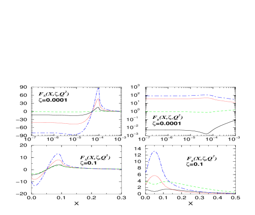
FIG. 2.: Unpolarized NLO input and evolved singlet quark and gluon GPDs at small and large skewedness. The solid curves are the input MRST99 GPDs at $Q_{0}=1~{}\mbox{GeV}$, the dotted ones show them evolved to $Q=10~{}\mbox{GeV}$. The dashed curves are input CTEQ5M GPDs at $Q_{0}=1~{}\mbox{GeV}$ and the dashed-dotted ones show them evolved to $Q=10~{}\mbox{GeV}$. The quark singlet is scaled by a factor of $10^{-4}$ at $\zeta=0.0001$ and by $10^{-2}$ at $\zeta=0.1$. For $\zeta=0.1$ the symmetry of the gluon GPD and the anti-symmetry of the singlet quark GPD are apparent about the point $X=\zeta/2=0.05$.

In Fig.(2) we plot the input distributions for the “new” unpolarized inputs (CTEQ5M and MRST99) at their input scale, and at an evolved scale to demonstrate the evolution effects in NLO.

IV DVCS amplitudes

A Convolution formulae

In [24] we investigated unpolarised and polarised DVCS amplitudes in detail. For convenience in the following equations we introduce the notation $V$ for the unpolarized case and $A$ for the polarized case, where applicable, they take the upper and lower signs, respectively. The factorization theorem [6, 7] for DVCS proves that the amplitude takes the following factorized form in the non-diagonal representation (up to power-suppressed corrections of ${\cal O}(1/Q)$):

$${\cal T}^{S,V/A}_{DVCS}(\zeta,\mu^{2},Q^{2},t)=\sum_{a}e^{2}_{a}\left(\frac{2-\zeta}{\zeta}\right)\Big{[} \int^{1}_{0}dX~{}T^{S(a),V/A}\left(\frac{2X}{\zeta}-1+i\epsilon,\frac{Q^{2}}{\mu^{2}}\right)~{}{\cal F}^{S(a),V/A}(X,\zeta,\mu^{2},t)$$ (50)

$$\Big{.}\mp \int^{1}_{\zeta}dX~{}T^{S(a),V/A}\left(1-\frac{2X}{\zeta},\frac{Q^{2}}{\mu^{2}}\right)~{}{\cal F}^{S(a),V/A}(X,\zeta,\mu^{2},t)\Big{]},$$ (51)

$${\cal T}^{g,V/A}_{DVCS}(\zeta,\mu^{2},Q^{2},t)=\frac{1}{N_{f}}\left(\frac{2-\zeta}{\zeta}\right)^{2}\Big{[} \int^{1}_{0}dX~{}T^{g,V/A}\left(\frac{2X}{\zeta}-1+i\epsilon,\frac{Q^{2}}{\mu^{2}}\right)~{}{\cal F}^{g,V/A}(X,\zeta,\mu^{2},t)$$ (52)

$$\pm\Big{.} \int^{1}_{\zeta}dX~{}T^{g,V/A}\left(1-\frac{2X}{\zeta},\frac{Q^{2}}{\mu^{2}}\right)~{}{\cal F}^{g,V/A}(X,\zeta,\mu^{2},t)\Big{]}\,.$$ (53)

Note that the second integral is purely real and does not need a $+i\epsilon$ prescription since there is no divergence of the coefficient function in the integration interval. Also note the opposite sign structure in the quark singlet and gluon case due to opposite symmetries of the quark singlet and gluon. For our numerical calculations, we set the factorization scale, $\mu^{2}$, equal to the photon virtuality, $Q^{2}$ (in [24] we studied the effects of its variation and found them to be rather mild; the associated uncertainties are less than those due to differences in the input model GPDs so we neglect them). Henceforth, we suppress the factorized $t$-dependence and give predictions for $t=0$. We will specify it for each case later. The LO and NLO coefficient functions, $T^{i,V/A}$, are taken from eqs.(14-17) of [44] and are summarized in appendix A of [24]. They contain logarithms of the type $\log(1-X/\zeta)^{n}/(1-X/\zeta)^{n_{1}}$, with $n,n_{1}=0,1,2,3$. Hence, depending on the region of integration, they can have both real and imaginary parts (i.e. if the argument of the log is positive or negative), which in turn generate real and imaginary parts of the DVCS amplitudes.

In eq.(53), we employ the $+i\epsilon$ prescription through the Cauchy principal value prescription (“P.V.”) which we implemented through the following algorithm:

$$\Big{.}P.V.\int^{1}_{0}dX~{}T\left(\frac{2X}{\zeta}-1\right){\cal F}(X,\zeta,Q^{2})=\int^{\zeta}_{0}dX~{}T\left(\frac{2X}{\zeta}-1\right)\left({\cal F}(X,\zeta,Q^{2})-{\cal F}(\zeta,\zeta,Q^{2})\right)+$$ (54)

$$\quad\quad\int^{1}_{\zeta}dX~{}T\left(\frac{2X}{\zeta}-1\right)\left({\cal F}(X,\zeta,Q^{2})-{\cal F}(\zeta,\zeta,Q^{2})\right)+{\cal F}(\zeta,\zeta,Q^{2})\int^{1}_{0}dX~{}T\left(\frac{2X}{\zeta}-1\right)\,.$$ (55)

Each term in eq. (55) is now either separately finite or only contains an integrable logarithmic singularity. This algorithm closely resembles the implementation of the $+$ regularization in the evolution of PDFs and GPDs. We note that the first integral (in the ERBL region) is strictly real. The second and third terms contain both real and imaginary parts (which are generated in the DGLAP region). Explicit expressions for the real and imaginary parts of the DVCS amplitudes are given in Sec.(II) of [24]. They involve integrals over the coefficient functions which may be calculated explicitly and are given in Appendix B of [24]. The real and imaginary parts of the unpolarized and polarized DVCS amplitudes were computed using a FORTRAN code based on numerical integration routines. We implemented the exact solution to the RNG equation for $\alpha_{s}$ in LO or NLO in our calculation, as appropriate, to be consistent throughout our analysis.

B Numerical results: unpolarized case

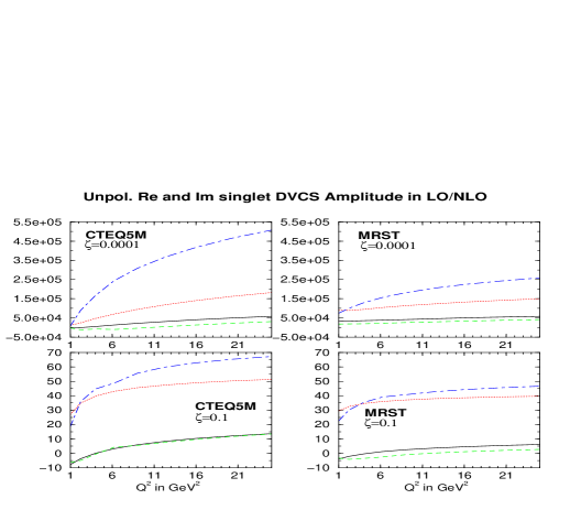
FIG. 3.: The $Q^{2}$-dependence of the real and imaginary parts of the quark singlet DVCS amplitude. The solid (dashed) curve is the real part in LO (NLO) and the dotted (dashed-dotted) curve is the imaginary part in LO (NLO).

In this subsection we illustrate the $Q^{2}$- and $\zeta$-dependence, as well as the size, of the real and imaginary parts of the unpolarized DVCS amplitudes for the new input distributions (MRST99, CTEQ5M), calculated at LO and NLO accuracy. Fig. 3 shows the $Q^{2}$-dependence of the real and imaginary parts of the quark singlet contribution, at LO and NLO, for two values of $\zeta=0.1,0.0001$, representative of HERMES and HERA kinematics, respectively. Correspondingly, Fig. 4 shows the gluon contributions, which start at NLO. Note the strong $Q^{2}$-dependence in NLO of the imaginary part of the quark singlet and gluon amplitude at small $\zeta$. This might raise concerns about the convergence of the perturbative expansion, especially when comparing NLO with LO in the quark singlet, where NLO grows much stronger with $Q^{2}$ than LO. This is due to the same type of logarithmic divergences as $X\to\zeta$ in both the evolution kernels and NLO coefficient functions. These divergences enhance the region around $\zeta$, which is important for the value of the imaginary part [23], more quickly in $Q^{2}$ than $\alpha_{s}$ drops as $Q^{2}$ increases. However, the quark singlet amplitude itself is not an observable quantity at NLO but rather the sum of quark singlet and gluon. When comparing the physical amplitudes at LO and NLO, the relative NLO corrections decrease as $Q^{2}$ increases, as they indeed should [23].

The above figures are complemented by Figs. 5 and Figs. 6, which show the $\zeta$-dependence at fixed $Q^{2}$ for the quark singlet and gluon contributions, respectively. Again we would like to point out the remarkable power-like behavior of the unpolarized amplitudes in $\zeta$ for fixed $Q^{2}$ already remarked upon and explained in [24] (with the exception of the NLO real parts of the quark singlet amplitude for CTEQ5M for the $Q^{2}$ values plotted due to a somewhat strange combination of small quark input and comparatively large gluon input. At higher $Q^{2}$, the CTEQ5M distribution also displays the characteristic power-like behavior in $\zeta$).

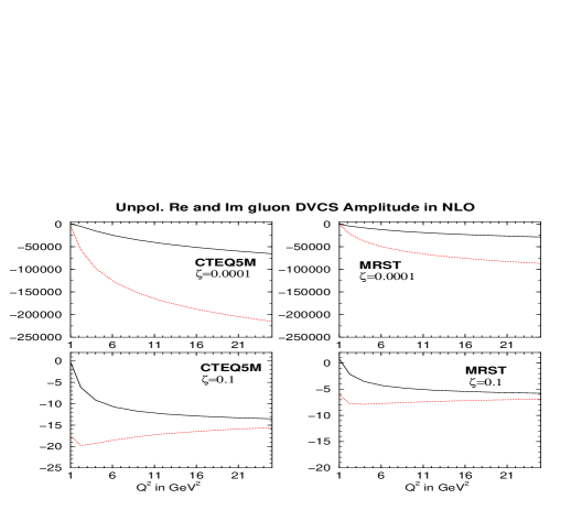
FIG. 4.: The $Q^{2}$-dependence of the real (solid line) and imaginary (dotted line) parts of the unpolarized gluon DVCS amplitude, which starts at NLO, for two representative values of $\zeta$.

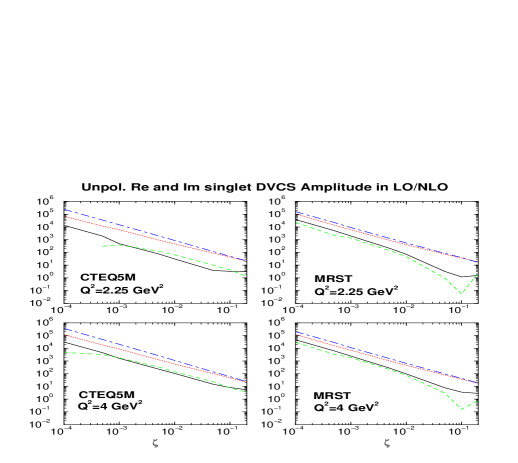
FIG. 5.: The real and imaginary parts of the unpolarized quark singlet DVCS amplitude, as a function of $\zeta$. The solid (dashed) curve is the real part in LO (NLO) and the dotted (dashed-dotted) curve is the imaginary part in LO (NLO). To be able to plot the NLO real part of the quark singlet amplitude in a viewable manner, we removed the first point for CTEQ5M in the upper left plot (since it was negative and thus not easily handled in a log-log plot) and shifted the NLO curve of the real part in the upper right plot upward by an amount of ${\cal O}(1)$, again to avoid negative numbers.

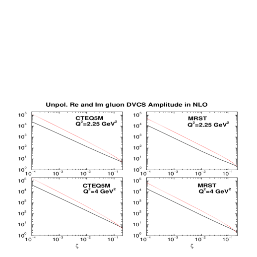
FIG. 6.: The real and imaginary parts of the unpolarized gluon DVCS amplitude as functions of $\zeta$, for fixed $Q^{2}$. The solid curve is the modulus of the real part (which is actually negative) and the dotted curve is the modulus of the imaginary part of the gluon amplitude, which is also negative!

C Specification of $t$-dependence and helicity flip amplitudes

In this subsection we specify the $t$-dependence of the various unpolarized/polarized helicity non-flip/flip DVCS amplitudes, ${\cal H}_{1},\widetilde{{\cal H}_{1}},{\cal E}_{1},\widetilde{{\cal E}}_{1}$, for each parton species $a=S(a=u,d,s),g$. These are required in eqs.(5, 6, 7) to fully specify ${\cal T}_{\mbox{{DVCS}}}$ (our choices follow those of [31] closely) . The various form factors are specified as follows:

$${\cal H}_{1}^{a}(\zeta,Q^{2},t)=F^{a}_{1}(t){\cal T}^{a,V}(\zeta,Q^{2})\,,~{}\qquad~{}{\cal{\tilde{H}}}_{1}^{a}(\zeta,Q^{2},t)=G^{a}_{1}(t){\cal T}^{a,A}(\zeta,Q^{2})\,,$$ (56)

$${\cal E}_{1}^{a}(\zeta,Q^{2},t)=F^{a}_{2}(t){\cal T}_{{\cal E}_{1}}^{a,V}(\zeta,Q^{2})\,,~{}\qquad~{}{\cal{\tilde{E}}}_{1}^{a}(\zeta,Q^{2},t)=G^{a}_{2}(t){\cal T}_{{\tilde{\cal E}}_{1}}^{a,A}(\zeta,Q^{2})\,,$$ (57)

where, in the helicity flip case on the second line, we have introduced additional subscripts, ${\cal E}_{1},{\tilde{\cal E}}_{1}$, on the right hand side to distinguish this case from the helicity non-flip one considered explicitly above. For the up and down quark flavors we exploit the fact that proton and neutron form an iso-spin doublet to arrive at:

$$2F^{u}_{i}(t)=2F^{p}_{i}(t)+F^{n}_{i}(t),~{}\qquad~{}2F^{d}_{i}(t)=F^{p}_{i}(t)+2F^{n}_{i}(t)\,,~{}\qquad~{}\mbox{for}\,~{}i=1,2\,,$$ (58)

corresponding to the Dirac and Pauli form factors, respectively (see eqs.(13, 14)). For the helicity non-flip polarized case we choose [31]:

$$G^{u,d}_{1}(t)=\left(1-\frac{t}{m^{2}_{A}}\right)^{-2}\,,\qquad G^{s,g}_{1}(t)=(1-\frac{t}{m_{A}^{2}})^{-3}\,,$$ (59)

where $m_{A}=0.9~{}\mbox{GeV}$ [33]. The strange quark and the gluon sea-like form factors were chosen in [31] using the counting rules for elastic form factors which give $1/t^{3}$, for large $t$. Hence, for the unpolarized case the electric and magnetic form factors were chosen to be

$$G^{s,g}_{E}(t)=\frac{G^{s,g}_{M}(t)}{1+\kappa^{s,g}}=\left(1-\frac{t}{m^{2}_{V}}\right)^{-3}\,,$$ (60)

where we further assume $\kappa^{s,g}=0$. This gives (cf. eq.(13))

$$F^{s,g}_{1}(t)=G_{E}^{s,g}(t)=\left(1-\frac{t}{m_{V}^{2}}\right)^{-3}\,,~{}\qquad~{}F^{s,g}_{2}(t)=0\,,$$ (61)

with $m_{V}=0.84$ GeV.

For the helicity-flip case, we still have to specify the polarized and unpolarized GPDs. Unfortunately there are no inclusive analogs to guide us. However, we do know that the unpolarized helicity flip GPD contains a D-term with a relative minus sign as compared to the helicity non-flip GPD, such that when added they cancel . In contrast to [31] we set the GPD equal to this D-term, which is non-zero only in the ERBL region. We then evolve this distribution in $Q^{2}$ and use it as an input to calculate ${\cal T}_{{\cal E}_{1}}^{a,V}$ for use in eq.(57), with the $F_{2}^{a}(t)$ for various $a$ specified in eqs.(58, 61).

For the polarized helicity flip amplitude, ${\cal T}_{\cal{\tilde{E}}}$, it was observed that, in a similar fashion to the effective pseudo scalar form factors in $\beta$-decay [33], one can approximate it at small $t$ by the pion pole (see for example [40]). Thus we chose the corresponding GPD to only contain the asymptotic pion distribution amplitude given by

$$\phi_{\pi}(X/\zeta)=\frac{8}{3}\frac{2-\zeta}{\zeta}\frac{X}{\zeta}\left(1-\frac{X}{\zeta}\right)\,,$$ (62)

in the ERBL region (and zero for $X>\zeta$). Since we use the asymptotic form we do not evolve the GPD and use it directly in the computation of the DVCS amplitude, ${\cal T}_{{\tilde{\cal E}}_{1}}^{a,A}(\zeta,Q^{2})$. The $t$-dependence is given by the pion pole and thus we find

$${\cal{\tilde{E}}}_{1}^{a}(\zeta,Q^{2},t)=G_{2}^{a}(t)~{}{\cal T}_{{\tilde{\cal E}}_{1}}^{a,A}(\zeta,Q^{2})=\frac{4g^{(3)}_{A}M^{2}}{m_{\pi}^{2}-t}{\cal T}_{{\tilde{\cal E}}_{1}}^{a,A}(\zeta,Q^{2})\,,~{}\qquad\,\mbox{for}\,~{}a=u,d\,,$$ (63)

where $g_{A}^{(3)}=1.267$, $M$ is the nucleon mass and ${\cal T}_{{\tilde{\cal E}}_{1}}^{a,A}=\phi_{\pi}$, for all $Q^{2}$. For the s-quark and the gluon we set $\tilde{\cal E}$ to zero. This completes the specification of the $t$-dependence of DVCS amplitudes, which are then used to compute the various DVCS observables defined in Sec. II.

We close this section with a few comments. We note that ${\cal E}_{1},{\cal{\tilde{E}}}_{1}$ only have real parts since the GPD is zero for $X>\zeta$. Furthermore, in the asymptotic limit $Q^{2}\to\infty$ for finite $\zeta$, when all the partons have accumulated in the ERBL region, all amplitudes have zero imaginary part and a real part which is given by an asymptotic distribution amplitude in the ERBL region, thus the overall amplitude, and hence the appropriately scaled triple differential cross section, remain non-zero, in contrast to inclusive DIS.

V LO and NLO results for DVCS observables

In this section we present results for the triple differential cross section and for various asymmetries (AAA, SSA, CA, UPLT, CADSFL) defined in subsection II B, in kinematics appropriate for the H1, ZEUS and HERMES experiments. We show the results as functions of $t$ (for fixed $\zeta,Q^{2}$), of $\zeta$ (for fixed $t,Q^{2}$) and of $Q^{2}$ (for fixed $t,\zeta$) using the various input distributions defined in subsection III B. For our predictions in HERA kinematics we assume an $e^{+}P$ scattering with a proton energy of $920$ GeV and a positron energy of $27.5$ GeV (except of course for the charge asymmetries, which also use an electron probe of $27.5$ GeV).

A The triple differential cross section

In Fig. 7 and Fig. 8 we show the triple differential cross section of eq.(19), as a function of $t$ at fixed $\zeta$ and $Q^{2}$, for our four input distributions. We note that at the common point $Q^{2}=4$ GeV², GRV98, MRSA’ and MRST99 are in close agreement, for small $\zeta=x$. In general CTEQ5M and MRST99 experience only moderate changes in going from LO to NLO.

At small $\zeta=x$, for GRV98 and MRSA’ input distributions, the NLO corrections are much larger. As $Q^{2}$ increases, at fixed $\zeta$, the spread of the predictions is seen to decrease. This is partly due to the evolution washing out the differences between the various input distributions, and partly due to an increased significance of the BH process.

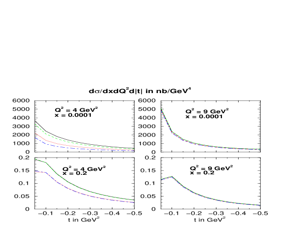
FIG. 7.: The triple differential cross section in $t$ for fixed $x=\zeta$ and $Q^{2}$. The solid (dotted) curve is the MRSA${}^{{}^{\prime}}$ set in LO (NLO) and the dashed (dashed-dotted) curve is the GRV98 set in LO (NLO).

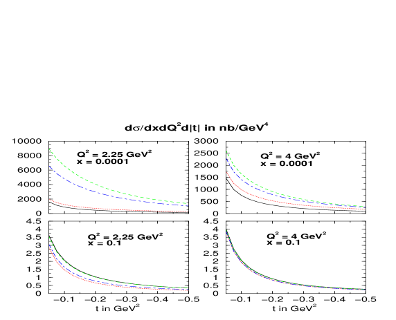
FIG. 8.: The triple differential cross section in $t$ for fixed $x=\zeta$ and $Q^{2}$. The solid (dotted) curve is the CTEQ5M set in LO (NLO) and the dashed (dashed-dotted) curve is the MRST99 set in LO (NLO).

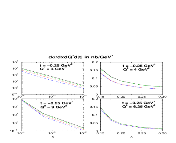
FIG. 9.: The triple differential cross section in $x=\zeta$ for fixed $t$ and $Q^{2}$. The solid (dotted) curve is the MRSA${}^{{}^{\prime}}$ set in LO (NLO) and the dashed (dashed-dotted) curve is the GRV98 set in LO (NLO).

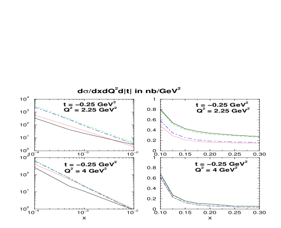
FIG. 10.: The triple differential cross section in $x=\zeta$ for fixed $t$ and $Q^{2}$. The solid (dotted) curve is the CTEQ5M set in LO (NLO) and the dashed (dashed-dotted) curve is the MRST99 set in LO (NLO).

In Figs. 9, 10, we employ logarithmic scales for HERA kinematics ($x<10^{-2}$) to illustrate the $\zeta$-behavior for fixed $Q^{2}$ and $t$. It is interesting to note that we find the same type of power law behavior, $\zeta^{n}$, for the triple differential cross section, which also includes the BH process, as we found previously for the unpolarized DVCS amplitudes (see Figs. 5 -6). Note that the kink for $Q^{2}=9~{}\mbox{GeV}^{2}$ is due to going from a BH dominated region at $x=0.0001$ ($y>0.8$) to a region where DVCS dominates ($x>0.0005$ and $y<0.2$).

The fact that the GRV98 and MRSA’ input scale is $Q_{0}^{2}=4$ GeV², implies that the available $Q^{2}$-range at small $x$ is rather limited for these distributions. Hence, in Fig. 11 we show only the $Q^{2}$-dependence of the MRST99 and CTEQ5M sets, which start at $Q_{0}^{2}=1$ GeV². For smaller $Q^{2}$, where DVCS dominates BH, the cross section falls quickly with $Q^{2}$ and one is sensitive to the details of the choice of input distribution. As $Q^{2}$ increases and BH starts to dominate over DVCS, one observes that the curves begin to converge and one loses sensitivity to the details of the input GPD.

We would like to point out that at large $x$ all of the distributions produce fairly similar results and that the NLO corrections are tame. This is expected because each of the distributions have been strongly constrained by global fits to high statistics data in this region and hence behave similarly. Any observed differences may result in part from the holistic nature of the GPDs, which requires a continuous function for all $X$, both at the input scale and upon evolution. The real part of the amplitude is sensitive to an integral over the ERBL region $X<\zeta$ so one may have some residual sensitivity to the behavior at very small $X\ll\zeta$, particularly if this behavior is extreme. The imaginary part is strongly influenced by the behavior at $X=\zeta$ which in turn is constrained by a symmetry in the ERBL region. This sensitivity is further enhanced at smaller $\zeta$, where the input PDFs are not yet so well constrained by direct (mainly inclusive) measurements. Hence, we optimistically speculate that a detailed measurement of the differential cross section, at HERA, for relatively low $Q^{2}\approx 1-4$ GeV², could help to discriminate between different standard input PDFs.

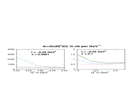
FIG. 11.: The triple differential cross section in $Q^{2}$ for fixed $t$ and $x=\zeta$. The solid (dotted) curve is the CTEQ5M set in LO (NLO) and the dashed (dashed-dotted) curve is the MRST99 set in LO (NLO).

B The single spin asymmetries (SSA,UPLT)

Having found a large spread of predictions for the triple differential cross section for different input GPDs, we now turn to two single spin asymmetries which are directly sensitive to the imaginary part of DVCS amplitudes. Let us first discuss the SSA, defined in eq.(22), which can be measured using a polarized lepton probe on an unpolarized target. At small $x$ the numerator in eq.(22) is directly proportional to $Im~{}{\cal H}_{1}$ (see the second term of eq.(30) of [31]).

In Figs. 12, 13 we illustrate the $t$-dependence at fixed $\zeta$ and $Q^{2}$, and note that the predictions range from as little as $5\%$ to as much as $30\%$. We note that in general the $t$-dependence is rather flat for $t>-0.1~{}\mbox{GeV}^{2}$, indicating that, to a certain extent, the $t$-dependence cancels in the ratio of eq.(22). This means that an experimental measurement of this asymmetry, even with a rather coarse binning in $t$, would be able to distinguish between different input scenarios, especially at larger $Q^{2}$ values. At the common scale of $Q^{2}=4$ GeV², the GRV98 and MRSA’ sets produce very similar numbers within LO and NLO, whereas CTEQ5M and MRST99 are more different within LO and NLO, at least at small $x$. The NLO to LO corrections are generally speaking small to moderate ($5-30\%$).

Figs. 14, 15 show that the SSA drops steeply in $\zeta=x$ for fixed $Q^{2}$ and $t$, suggesting that the HERA experiments will only be able to measure the SSA in the small $\zeta$ regime ($\zeta\in[10^{-3},10^{-4}]$). We would also like to point out that the differences for the different input sets becomes so small on the scale of the actual value of the SSA at larger $\zeta$ in HERA kinematics, that only very high statistics would be able to discriminate between them. Thus, for HERA, only a small $\zeta$ measurement would gives a reasonable discrimination between the various inputs. For HERMES kinematics, where for fixed $\zeta=x,Q^{2}$ one of course probes a different $y=Q^{2}/xS$ value, the SSA again becomes sizeable. Unfortunately, in this high $\zeta=x$ regime, the SSA is proportional to a linear combination of imaginary parts of ${\cal H}_{1},{\tilde{{\cal H}}_{1}},{\cal E}_{1}$ rather than just $Im~{}{\cal H}_{1}$ as at small $\zeta$ (see second term of eq.(30) of [31]).

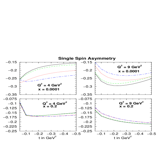
FIG. 12.: The single spin asymmetry as a function of $t$, for fixed $x=\zeta$ and $Q^{2}$. The solid (dotted) curve is the MRSA${}^{{}^{\prime}}$ set in LO (NLO) and the dashed (dashed-dotted) curve is the GRV98 set in LO (NLO).

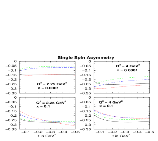
FIG. 13.: The SSA in $t$ for fixed $x$ and $Q^{2}$. The solid (dotted) curve is the CTEQ5M set in LO (NLO) and the dashed (dashed-dotted) curve is the MRST99 set in LO (NLO).

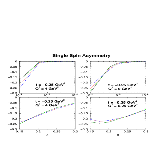
FIG. 14.: The SSA in $x=\zeta$ for fixed $t$ and $Q^{2}$. The solid (dotted) curve is the MRSA${}^{{}^{\prime}}$ set in LO (NLO) and the dashed (dashed-dotted) curve is the GRV98 set in LO (NLO).

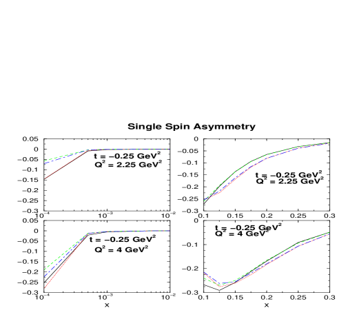
FIG. 15.: The SSA as a function of $x=\zeta$ for fixed $t$ and $Q^{2}$. The solid (dotted) curve is the CTEQ5M set in LO (NLO) and the dashed (dashed-dotted) curve is the MRST99 set in LO (NLO).

Finally, in Fig. 16 we plot the $Q^{2}$-dependence for fixed $\zeta=x$ and $t$. For small $\zeta$ we observe that the magnitude of the SSA increases with $Q^{2}$, for both distributions. At large $\zeta$, both MRST99 and CTEQ5M have very similar $Q^{2}$ behavior and the NLO corrections are small. Note that at small $\zeta$ the NLO corrections appear to grow in $Q^{2}$ which at first sight looks strange. This is due to the fact that the BH process gains prominence relative to the DVCS process, so any differences between calculations of $Im{\cal H}_{1}$ for the interference term in the numerator become enhanced. However, the NLO corrections remain moderate between $15-30\%$.

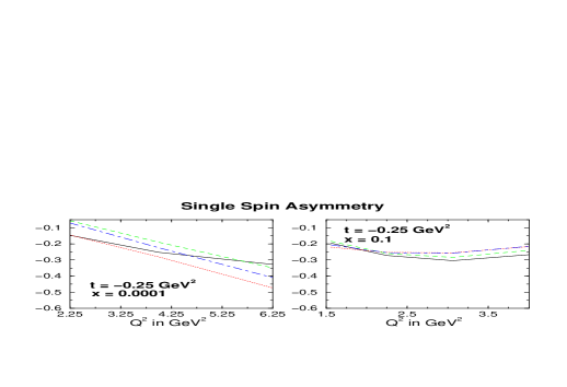
FIG. 16.: The SSA as a function of $Q^{2}$, for fixed $t$ and $x=\zeta$. The solid (dotted) curve is the CTEQ5M set in LO (NLO) and the dashed (dashed-dotted) curve is the MRST99 set in LO (NLO).

If one switches now to a longitudinally polarized proton target as available at HERMES, but not currently planned for HERA, and an unpolarized lepton probe, one can form the unpolarized single spin asymmetry UPLT which is directly sensitive to the imaginary part of a combination of DVCS amplitudes. Furthermore, for the small $\zeta$ regime within HERA kinematics, we find on inspection of the first term (proportional to $\Lambda\sin\phi$) of eq.(31) of [31] that the UPLT at small $\zeta$ is directly proportional to the imaginary part of the polarized amplitude ${\cal{\tilde{H}}}_{1}$ and that the other amplitudes like the numerically large ${\cal H}_{1}$ are suppressed by $x$. Hence, even though $Im~{}{\cal{\tilde{H}}}_{1}$ is about a factor of one thousand smaller than $Im~{}{\cal H}$ at $x=10^{-4}$, the suppression factor of $x$ means that $Im~{}{\cal H}_{1}$ constitutes only a $10\%$ correction. Hence the UPLT is mainly sensitive to $Im~{}{\cal{\tilde{H}}}_{1}$ at small $x$. Since this amplitude is numerically small, we found the UPLT asymmetry itself to be very small, at small $x=\zeta$, and thus virtually impossible to measure. Therefore, we do not show plots for HERA kinematics but rather only for HERMES kinematics.

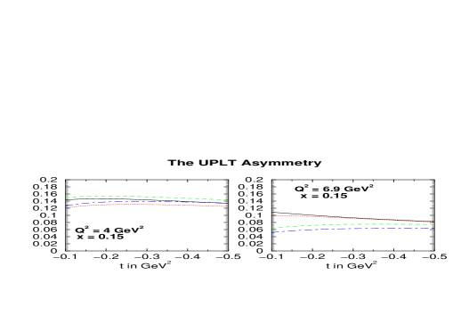
FIG. 17.: The UPLT as a function of $t$, for fixed $x$ and $Q^{2}$. The solid (dotted) curve is the MRSA${}^{{}^{\prime}}$ set in LO (NLO) and the dashed (dashed-dotted) curve is the GRV98 set in LO (NLO).

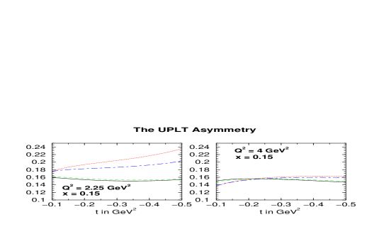
FIG. 18.: The UPLT as a function of $t$, for fixed $x$ and $Q^{2}$. The solid (dotted) curve is the CTEQ5M set in LO (NLO) and the dashed (dashed-dotted) curve is the MRST99 set in LO (NLO).

In Figs. 17 and 18, we show the UPLT as a function of $t$ for fixed $Q^{2}$ and $\zeta=x=0.15$, i.e. in HERMES kinematics, where $Im~{}{\cal H}$ and other amplitudes contribute significantly. Hence, despite the fact that this asymmetry should be measurable at HERMES, the results would only be useful in the context of a program of asymmetry measurements that would enable the individual DVCS amplitudes to be isolated. Again a rather flat behavior is observed in $t$. We observe that all sets agree well with one another and their NLO corrections are small, in terms of percentages. In Figs. 19, 20 we plot the UPLT as a function of $\zeta=x$ at fixed $t,Q^{2}$. Note the good agreement of all sets in the $Q^{2}=4~{}\mbox{GeV}^{2}$ figures. This agreement does not bode well for the usefulness of the UPLT to discriminate between different input models. The NLO effects are found to be generally small. Finally, in Fig. 21 we show that the $Q^{2}$-behavior of the UPLT asymmetry, is rather complicated (for the same reasons as in the case of the SSA in HERMES kinematics). Note the close agreement of all sets for the $Q^{2}>4~{}\mbox{GeV}^{2}$ behavior and the smallness of the NLO corrections.

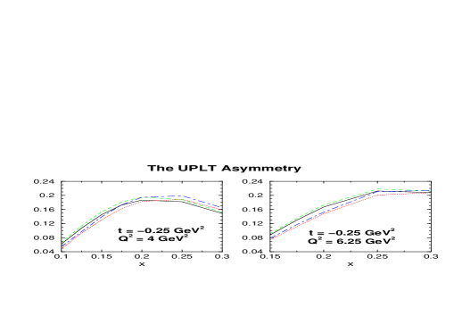
FIG. 19.: The UPLT as a function of $x=\zeta$, for fixed $t$ and $Q^{2}$. The solid (dotted) curve is the MRSA${}^{{}^{\prime}}$ set in LO (NLO) and the dashed (dashed-dotted) curve is the GRV98 set in LO (NLO).

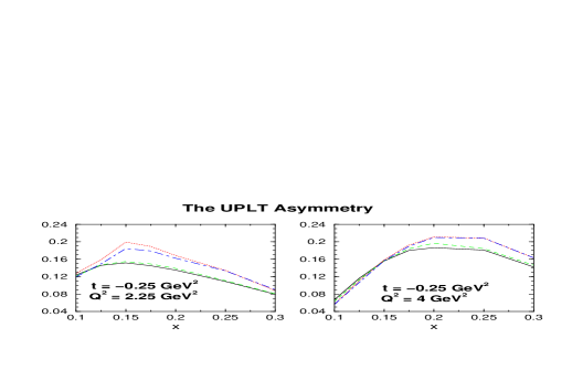
FIG. 20.: The UPLT as a function of $x=\zeta$, for fixed $t$ and $Q^{2}$. The solid (dotted) curve is the CTEQ5M set in LO (NLO) and the dashed (dashed-dotted) curve is the MRST99 set in LO (NLO).

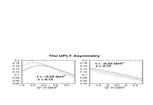
FIG. 21.: The UPLT as a function of $Q^{2}$, for fixed $t$ and $x=\zeta$. In the left figure, the solid (dotted) curve is the CTEQ5M set in LO (NLO) and the dashed (dashed-dotted) curve is the MRST99 set in LO (NLO), and in the right figure, the solid (dotted) curve is the MRSA’ set in LO (NLO) and the dashed (dashed-dotted) curve is the GRV98 set in LO (NLO).

C The azimuthal angle asymmetry (AAA)

We now discuss the (unpolarized) azimuthal angle asymmetry, defined in eq. (21), which directly probes the real part of DVCS amplitudes and only $Re~{}{\cal H}_{1}$ at small $\zeta=x$ where it dominates the other amplitudes (cf. the term proportional to $\cos\phi$ in eq.(30) of [31]). Again we would like to point out that subtracting the BH contribution is necessary since it does not cancel in the asymmetry due to the $\phi$-dependence of the propagators ${\cal P}_{1}$ and ${\cal P}_{2}$.

In general, Figs. 22, 23 reveal a rather flat behavior of the AAA in $t$, for fixed $\zeta,Q^{2}$. We note that the spread of predictions coming from different inputs is rather large, indicating a strong sensitivity of the AAA to the input distributions and to the order in perturbation theory. The NLO corrections are very large, simply because the gluon enters at NLO for the first time, with a relative minus sign compared to the quarks in the real parts of the amplitudes. The wide spread in results indicates that the AAA is a highly sensitive discriminator between different input models, even those which have, up until now, agreed very well with one another. Hence, measuring the AAA both at HERA and HERMES with high precision is imperative for constraining the GPDs via a global fit. Note also that this strong sensitivity to the details of the shape and size of the GPD both in the ERBL and DGLAP region, as anticipated by the results in [23, 24], indicates that an extraction of the GPDs with reasonable precision may be possible.

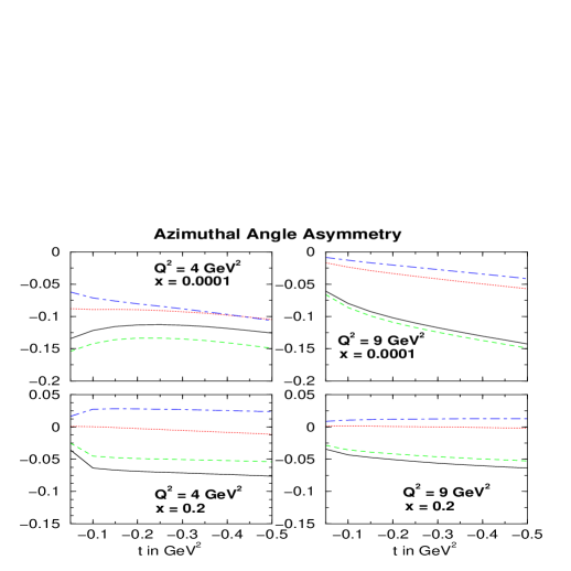
FIG. 22.: The AAA in $t$ for fixed $x=\zeta$ and $Q^{2}$. The solid (dotted) curve is the MRSA${}^{{}^{\prime}}$ set in LO (NLO) and the dashed (dashed-dotted) curve is the GRV98 set in LO (NLO).

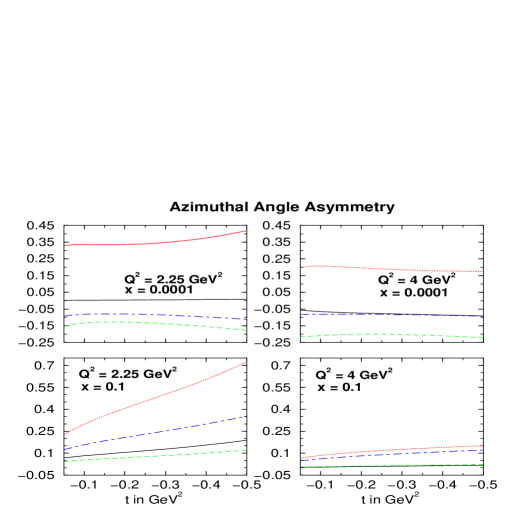
FIG. 23.: The AAA in $t$ for fixed $x=\zeta$ and $Q^{2}$. The solid (dotted) curve is the CTEQ5M set in LO (NLO) and the dashed (dashed-dotted) curve is the MRST99 set in LO (NLO).

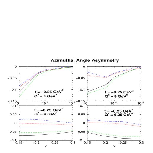
FIG. 24.: The AAA in $x=\zeta$ for fixed $t$ and $Q^{2}$. The solid (dotted) curve is the MRSA${}^{{}^{\prime}}$ set in LO (NLO) and the dashed (dashed-dotted) curve is the GRV98 set in LO (NLO).

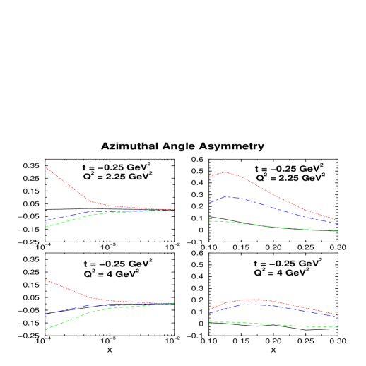
FIG. 25.: The AAA in $x=\zeta$ for fixed $t$ and $Q^{2}$. The solid (dotted) curve is the CTEQ5M set in LO (NLO) and the dashed (dashed-dotted) curve is the MRST99 set in LO (NLO).

Figs. 24 and 25 illustrate the strong decrease of the AAA as $\zeta$ decreases within HERA kinematics (i.e. small $\zeta$), for fixed $Q^{2},t$. However, as expected from dispersion relations, this behavior at small $\zeta$ of AAA, which is sensitive to $Re{\cal H}_{1}$, is naturally not as steep as that of SSA, which is sensitive to $Im{\cal H}_{1}$. Note again the kink at $Q^{2}=9~{}\mbox{GeV}^{2}$ when going from a BH dominated region to a DVCS dominated one, i.e. from high to low $y$.

The $\zeta$-dependence of the AAA in the valence region probed at HERMES (where it has already measured the SSA), shows very large NLO effects, consistent within all sets, which make the AAA large and thus measurable at HERMES. The large overall size and spread of predictions is encouraging for measurements of the AAA at large $x$ since even here the discriminating power between GPD models is very good.

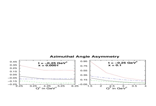
FIG. 26.: The AAA in $Q^{2}$ for fixed $t$ and $x=\zeta$. The solid (dotted) curve is the CTEQ5M set in LO (NLO) and the dashed (dashed-dotted) curve is the MRST99 set in LO (NLO).

Finally we show the $Q^{2}$-dependence of the AAA in Fig. 26 (again only for MRST99 and CTEQ5M, due to their lower input scale). For small $\zeta=x$ we see a fairly flat behavior of the AAA with $Q^{2}$ with the NLO to LO changes staying fairly constant in $Q^{2}$. At large $\zeta=x$, the predictions for the two sets quickly approach one another in both LO and NLO as $Q^{2}$ increases. Also the NLO to LO change decreases as $Q^{2}$ increases in line with the argument that BH starts dominating at large $Q^{2}$ due to the associated increase in $y$.

D The charge asymmetries (CA,CADSFL)

Other asymmetries which measure the real part of DVCS amplitudes are the charge and charge double spin flip asymmetries (see eqs.(25, 26)). These asymmetries require the measurement of DVCS with both the positron and the electron and, in the case of the CADSFL, a longitudinally polarized probe and target at the same time. Thus they are more difficult to measure than the AAA or other observables. The CA isolates the same combination of real parts of DVCS amplitudes as the AAA (i.e. the first term in eq.(30) of [31], which is proportional to $\cos\phi$), and would therefore serve as a useful complementary measurement.

The CADSFL isolates the combination of real parts of DVCS amplitudes given in the second term of eq.(31) of [31]. The UPLT asymmetry isolates the imaginary part of the same linear combination. Thus a combined measurement of both CADSFL and UPLT at small $x$ reveals information about the real and imaginary parts of the polarized helicity non-flip DVCS amplitude ${\cal{\tilde{H}}}_{1}$.

We discuss the CA first. Figs. 27-31 reveal that the CA is very similar to the AAA in the BH dominated region, and is within $20\%$ of it in the DVCS dominated region for both LO and NLO. It can be easily seen that the $t,x$ and $Q^{2}$ behavior is very similar for both asymmetries. This behavior can be understood quite easily: in contrast to the AAA case, for CA the interference term drops out in the normalization in eq. (25) due to the sign change of the interference term in going from a positron to an electron probe. The numerator is the same for both asymmetries. Hence, deviations between the AAA and the CA results show directly the influence of the interference term relative to the BH and DVCS contributions. The larger the deviation the more important the interference term. Hence, a precise measurement of the CA and the AAA will serve as a very good consistency check of the experimental analysis, since strong deviations between the CA and AAA are not expected. One caveat here is the possible importance of higher twist contributions in the interference term.

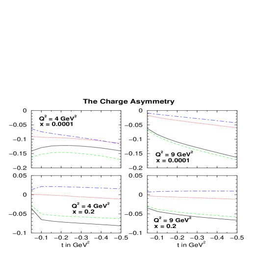
FIG. 27.: The CA in $t$ for fixed $x=\zeta$ and $Q^{2}$. The solid (dotted) curve is the MRSA${}^{{}^{\prime}}$ set in LO (NLO) and the dashed (dashed-dotted) curve is the GRV98 set in LO (NLO).

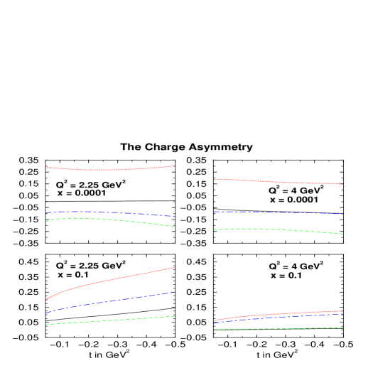
FIG. 28.: The CA in $t$ for fixed $x=\zeta$ and $Q^{2}$. The solid (dotted) curve is the CTEQ5M set in LO (NLO) and the dashed (dashed-dotted) curve is the MRST99 set in LO (NLO).

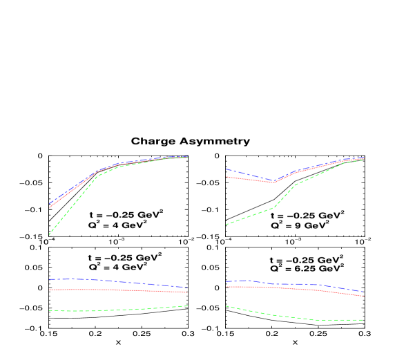
FIG. 29.: The CA in $x=\zeta$ for fixed $t$ and $Q^{2}$. The solid (dotted) curve is the MRSA${}^{{}^{\prime}}$ set in LO (NLO) and the dashed (dashed-dotted) curve is the GRV98 set in LO (NLO).

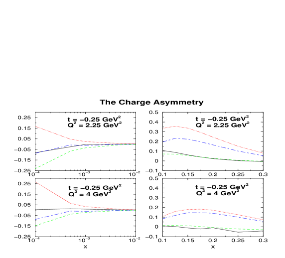
FIG. 30.: The CA in $x=\zeta$ for fixed $t$ and $Q^{2}$. The solid (dotted) curve is the CTEQ5M set in LO (NLO) and the dashed (dashed-dotted) curve is the MRST99 set in LO (NLO).

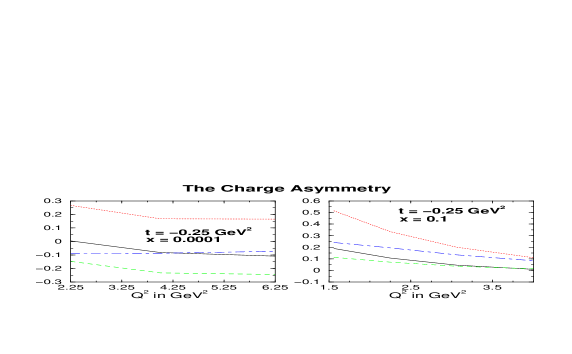
FIG. 31.: The CA in $Q^{2}$ for fixed $t$ and $x=\zeta$. The solid (dotted) curve is the CTEQ5M set in LO (NLO) and the dashed (dashed-dotted) curve is the MRST99 set in LO (NLO).

Moving now to a longitudinally polarized probe and target, we will study the charge asymmetry in a double spin flip experiment, the CADSFL.

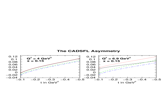
FIG. 32.: The CADSFL in $t$ for fixed $x=\zeta$ and $Q^{2}$. The solid (dotted) curve is the MRSA${}^{{}^{\prime}}$ set in LO (NLO) and the dashed (dashed-dotted) curve is the GRV98 set in LO (NLO).

For HERA kinematics the CADSFL turns out to be too small to be measured, i.e. consistent with zero for any practical purposes, and thus we will not show plots for HERA kinematics. For HERMES kinematics, the asymmetry is of the order of a few percent, so one might hope to be able to measure it. In Figs. 32 and 33 we show the $t$-dependence for fixed $\zeta=x$ and $Q^{2}$, which turns out to be rather steep. In Figs. 34 and 35 we show the $\zeta$-dependence for fixed $t,Q^{2}$. They indicate that although in percentage terms the spread of predictions is large the overall size of the CADSFL (only a few percent) would seem to indicate that exploiting this spread of predictions is impractical.

Finally we show the $Q^{2}$-behavior of CADSFL in Fig. 36, for fixed $t,\zeta$. We see quite a moderate to large difference in going from LO to NLO. Note the sign difference between the GRV98 and MRSA’ sets on the one hand and the CTEQ5M and MRST99 sets on the other hand. This gives some hope to use this asymmetry as a discriminator between different model inputs. Generally speaking, due to its overall smallness, it is not as promising a candidate as the CA asymmetry as a good DVCS observable, even though it is directly sensitive to the real part of a polarized amplitude at small $\zeta$. This concludes our presentation of DVCS observables in LO and NLO.

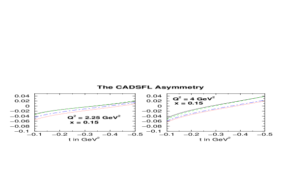
FIG. 33.: The CADSFL in $t$ for fixed $x=\zeta$ and $Q^{2}$. The solid (dotted) curve is the CTEQ5M set in LO (NLO) and the dashed (dashed-dotted) curve is the MRST99 set in LO (NLO).

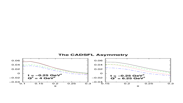
FIG. 34.: The CADSFL in $x=\zeta$ for fixed $t$ and $Q^{2}$. The solid (dotted) curve is the MRSA${}^{{}^{\prime}}$ set in LO (NLO) and the dashed (dashed-dotted) curve is the GRV98 set in LO (NLO).

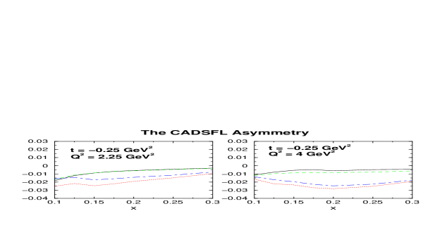
FIG. 35.: The CADSFL in $x=\zeta$ for fixed $t$ and $Q^{2}$. The solid (dotted) curve is the CTEQ5M set in LO (NLO) and the dashed (dashed-dotted) curve is the MRST99 set in LO (NLO).

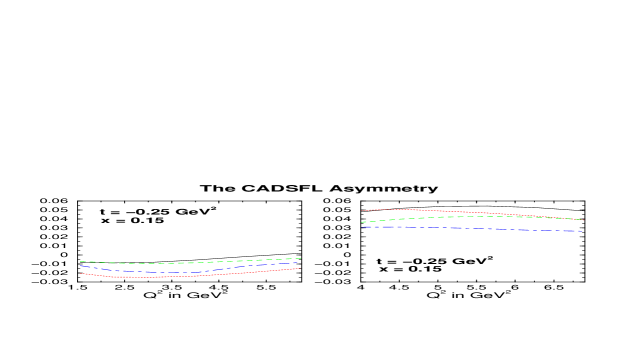
FIG. 36.: The CADSFL in $Q^{2}$ for fixed $t$ and $x=\zeta$. In the left figure, the solid (dotted) curve is the CTEQ5M set in LO (NLO) and the dashed (dashed-dotted) curve is the MRST99 set in LO (NLO), and in the right figure, the solid (dotted) curve is the MRSA’ set in LO (NLO) and the dashed (dashed-dotted) curve is the GRV98 set in LO (NLO).

E Summary of optimal DVCS observables

We summarise the results of the previous subsections as follows:

• The triple differential cross section is quite a good discriminator between different GPD models, particularly at $Q^{2}$ values close to the input scale (at higher $Q^{2}$ the BH process dominates). We predict a steep rise with decreasing $\zeta$ reflecting the underlying powerlike behavior in $\zeta$ of the DVCS amplitudes.

• The SSA is quite sizable and well behaved in NLO for all the input GPDs concerned, which makes it a very good candidate to be measured both at HERA and HERMES. For small $\zeta$ (HERA kinematics) we predict a strong increase in magnitude as $\zeta$ decreases (a feature shared by AAA and CA) and good discriminating power between input models, especially at larger $Q^{2}$.

• The AAA and CA seem to be very good candidates for discriminating between different input GPDs simply because they measure the real part of DVCS amplitudes which are very sensitive to the underlying details of the GPDs, in Radyushkin’s ansatz, especially at NLO where the gluon enters with a relative minus sign for the real part of its amplitude. Practical measurements for both asymmetries appear feasible for both HERMES and HERA kinematics.

• The measurement of UPLT (CADSFL) appears to be practical only at large $\zeta$ in HERMES kinematics, where it tests a linear combination of imaginary (real) parts of several DVCS amplitudes. Therefore these measurements have very limited discriminating power between model GPDs.

In summary it seems that four out of six observables are large enough to make measurements at HERA and HERMES feasible, and which have good discriminating power between input scenarios. Thus the prospects of unraveling the details of the DVCS process experimentally are in principle very good.

VI Comparison with experiment and other calculations

In this section we compare our LO and NLO results for each of our input sets with the available published experimental data from H1 and HERMES. The ZEUS collaboration announced the first measurement of DVCS at HERA [9] (see also [13]), but has yet to publish a cross section.

H1 recently published their data [10] on the measured DVCS cross section on both the lepton level and the photon level. They use the equivalent photon approach, which relates the pure DVCS cross section on the lepton level (with the interference neglected and the pure BH term subtracted) to the virtual-photon proton cross section:

$$\frac{d^{2}\sigma(ep\to ep\gamma)}{dydQ^{2}}=\Gamma~{}\sigma_{DVCS}(\gamma^{*}p\to\gamma p)~{}\qquad~{}\mbox{where}~{}~{}\qquad~{}\Gamma=\frac{\alpha_{e.m.}(1+(1-y)^{2})}{2\pi yQ^{2}}.$$ (64)

By integrating eq. (19) over $t,\phi$, and changing variables from $x_{bj}$ to $y$, we can establish the formula for the photon-level cross section in terms of our amplitudes as

$$\sigma_{DVCS}(\gamma^{*}p\to\gamma p)=\frac{\alpha^{2}x^{2}\pi}{Q^{4}{\cal B}}|{\cal T}_{DVCS}|^{2}|_{t=0},$$ (65)

where ${\cal B}$ stems from the $t$-integration and, within our model for the $t$-dependence, ${\cal B}\approx 6.5$ GeV^-2 (with a surprisingly small spread of about $1$ GeV^-2 !). We observed that for the kinematical region of the H1 data which is limited to small $x$, i.e. to small $\zeta$, we could write

$$\int^{t_{\mbox{{tmin}}}}_{-\infty}~{}dt~{}|{\cal T}_{DVCS}|^{2}\approx\frac{1}{{\cal B}}|{\cal T}_{DVCS}|^{2}|_{t=0}$$ (66)

as if we had assumed a global exponential dependence, $e^{Bt}$, as was used by H1 in their comparison to other [8, 46] calculations (dropping all amplitudes except ${\cal H}$). On numerical inspection we found that indeed ${\cal H}$ clearly dominates all the other amplitudes for HERA kinematics. Therefore, in comparing to the data, we can safely neglect all other amplitudes (i.e. polarised and helicity-flip) in the DVCS square term.

The same assumption was made in previous LO QCD [8] and two-component dipole model [46, 47] calculations, which both reproduce the H1 data quite well. Since ours is a QCD calculation we point out the differences and similarities with [8]. The latter was based on a LO input (CTEQ3L) with the assumption that the GPDs are equal to the PDFs at the input scale. The imaginary part of the unpolarized helicity non-flip amplitude was then computed using the aligned jet model and the imaginary part, rather than the GPD, was then evolved to higher $Q^{2}$. This is equivalent to what we did at LO since the imaginary part of the DVCS amplitude is simply $\pi$ times the GPD at $\zeta=x_{bj}$, legitimising the approach in [8]. The DVCS triple differential cross section, at small $x$, was then computed by comparing the imaginary part of DVCS to DIS and thus introducing the structure function $F_{2}$ through the optical theorem. In order to reconstruct the real part of the DVCS amplitude a dispersion relation approach was used which exploited the slope of $F_{2}$ in $\ln(1/x)$ at small $x$ (which was extracted from data to give $\eta=ReA_{\mbox{{DIS}}}/ImA_{\mbox{{DIS}}}$) together with the comparative factor $R=ImA_{\mbox{{DVCS}}}/ImA_{\mbox{{DIS}}}$. The specification was completed with the additional assumption of a global $t$-dependence, $e^{Bt}$. In contrast to [8], we computed both parts of the DVCS amplitudes directly and used them in the unapproximated expressions for the DVCS triple differential cross section, which also contains the polarized as well as helicity flip amplitudes (however these can be safely neglected in the cross section at small $\zeta$). Furthermore, we assumed a dipole type $t$-dependence which is close to the exponential behavior at small $\zeta$ and $t$, as well as being correct at larger $t$ (and small $\zeta$).

In Fig. 37 we plot $\sigma_{DVCS}(\gamma^{*}p)$ at $Q^{2}=4.5$ GeV² in $W$ (this is of course similar to a plot in $1/x=W^{2}/Q^{2}$) for GRV and MRST input models at LO and NLO. Also shown is the H1 data, for which they quote $<\!Q^{2}\!>=4.5$ GeV², with systematic and statistical error bars added in quadrature. In Fig. 38, we plot $\sigma_{DVCS}(\gamma^{*}p)$ in $Q^{2}$ for fixed $W=75$ GeV. The most obvious observation to make is that all of the the curves lie well above the data. However they do have the correct shapes (rising with $W$ and falling rapidly with $Q^{2}$).

FIG. 37.: The photon level cross section $\sigma(\gamma^{*}P\to\gamma P)$ as a function of  $W$ at fixed $Q^{2}=4.5$ GeV², for GRV98 and MRST99 at LO and NLO. Also shown are the recent H1 data, at $Q^{2}=4.5$ GeV², with systematic and statistical errors added in quadrature.

FIG. 38.: The photon level cross section $\sigma(\gamma^{*}P\to\gamma P)$ as a function of $Q^{2}$ at fixed $W=75$ GeV, for GRV98 and MRST99 at LO and NLO. Also shown are the recent H1 data, at $W=75$ GeV, with systematic and statistical errors added in quadrature.

In order to understand this discrepancy we re-examined Radyushkin’s input model in detail. For the unpolarized gluon GPD in [23] we found a rather moderate enhancement of about $20\%$ of the GPD relative to the forward case at the point $X=\zeta$. However, for the quark singlet, in which $q$ rather than $xq$ is used in the double distributions, we found this enhancement to be as large as a factor four! Such a large enhancement stems from the fact that the quark singlet distributions from the chosen input GPDs are very singular in the small $x$ region ($q(x)\propto x^{-1-\lambda}$ ), and therefore lead to an integrable singularity in the double distribution at $x^{\prime}=0$ (the shape function for the quark singlet is $\propto x$ for $x\rightarrow 0$ and this reduces the degree of the singularity to an integrable one). This leads to a large enhancement close to $X=\zeta$ and a strong and unsatisfactory sensitivity to the extrapolation of the input PDFs to very small $x$, where they have not yet been measured (cf. eqs.(40,41)). This is clearly a very unsatisfactory behaviour from a physical point of view and thus we are led to conclude that Radyushkin’s input model should be used only with non-singular inputs.

To illustrate the strong sensitivity of the results to the particular choice of input GPD we make a very simple change to the input model, namely we shift the argument of the PDFs in eq.(14) of [21] from $x$ to $x+\zeta$. This (admittedly rather ’ad hoc’) modification, which we make purely for the purpose of demonstration, preserves the symmetries in the ERBL region and the forward limit, but can be expected to spoil the polynomiality properties, which are then restored under evolution [45]. In making this modification we ensure that the PDFs are never sampled below $x=\zeta$ (which removes the sensitivity to the very small $x$ region) and can be expected to reduce considerably the enhancement of the GPDs at $X=\zeta$. Figs. 39 and 40 show the very dramatic effect on the cross section. The theory curves for the modified ansatz now undershoot the experimental data by about a factor of two and appear to reproduce the shape in $W$ and $Q^{2}$ rather well. In summary we claim that this illustrates that the H1 data are already able to begin to constrain the input GPDs. It seems clear that if one is to use Radyushkin’s ansatz at very small $\zeta$ the input PDFs should be non-singular. Alternatively, one must invent a new parameterization of the GPDs at the input scale that retains the required features (correct polynomiality and symmetry properties and faithful reproduction of the forward limit) without the problem of a strong sensitivity to the very small $x$ region and associated large enhancement of the GPDs relative to the PDFs at the point $X=\zeta$. This might be achieved by choosing a non-singular double distribution at a very low input scale, with the small $X$ behavior generated by perturbative evolution.

FIG. 39.: The photon level cross section $\sigma(\gamma^{*}P\to\gamma P)$ as a function of $W$ at $Q^{2}=4.5$ GeV², for GRV98 and MRST99 at LO and NLO using the shifted ansatz.

FIG. 40.: The photon level cross section $\sigma(\gamma^{*}P\to\gamma P)$ as a function of $Q^{2}$ at fixed $W=75$ GeV, for GRV98 and MRST99 at LO and NLO, using the shifted ansatz.

We now turn to the SSA as measured by the HERMES collaboration [11]. They define the SSA, weighted with $\sin\phi$, as follows:

$$SSA=\frac{2\int_{0}^{2\pi}d\phi~{}\sin\phi~{}(d\sigma^{\uparrow}-d\sigma^{\downarrow})}{\int_{0}^{2\pi}(d\sigma^{\uparrow}+d\sigma^{\downarrow})}\,.$$ (67)

They quote two values: $SSA=-0.18\pm 0.05\pm 0.05$ and $\langle SSA\rangle=-0.23\pm 0.03\pm 0.04$. The first, which assumes that their missing mass equals the proton mass, is quoted at the following average values: $<\!x\!>=0.11,<\!Q^{2}\!>=2.5$ GeV² and $<\!t\!>=-0.27$ GeV². The second (average) value is the SSA integrated over the missing mass at the same average values of $x,Q^{2}$ and $t$. At this point in $x,Q^{2},t$ for the HERMES definition we find $SSA=-0.365$ for CTEQ5M and $SSA=-0.35$ for MRST99.

Given the fact that the input models used do not describe the data at small $\zeta$, and that we find the same type of enhancement effect when comparing GPDs with forward PDFs at both small and large $\zeta$, the failure to describe the HERMES data is not surprising. In fact one needs higher statistics over a wide kinematic range in several DVCS observables to be able to begin to tune the input GPDs using a fitting method. Only then can one start discriminating between different choices for the PDFs in input models. Furthermore, for HERMES data one needs to know the normalizations of numerator and the denominator producing the measured asymmetry to help to constrain the normalization of the individual amplitudes (in order to be able to make any sensible statements about a comparison between theory and experiment).

In comparing with other calculations we show qualitative agreement with [8, 46, 47] and quantitative agreement with [31, 44] wherever we used the same input distributions (MRSA’ and GS(A) only).

VII Conclusions

We have presented a detailed next-to-leading (NLO) QCD analysis of deeply virtual Compton scattering (DVCS) observables. We quantified the NLO corrections and established which observables have the best prospects to be measured accurately at HERA and HERMES (the triple differential cross section and the azimuthal angle (AAA), single spin (SSA) and charge (CA) asymmetries). We have demonstrated that such measurements would have good discriminating power between different scenarios for the generalized parton distributions (GPDs), by examining four cases. It turns out that AAA and CA, which test the real part of unpolarized DVCS amplitude at small $x$ are the most sensitive to the choice of GPD model.

We performed a comparison with presently available DVCS data and showed that within Radyushkin’s ansatz for the GPDs, all of the models we examined overshoot the H1 data. This is due to their singular nature of the quark singlet at small $x$ which leads to a strong sensitivity to the PDFs in the extremely small $x$ region, where they have not yet been measured. We illustrated this strong sensitivity by artificially shifting the argument of the PDFs by $\zeta$, which led to a large reduction in the theoretical predictions for the photon-level cross section (which then undershoots the data). This illustrates an urgent need for improved input models, which do not rely on a singular double distribution and also for more, high precision data to help constrain them.

REFERENCES

- [1] D. Müller et al., Fortsch. Phys. 42 (1994) 101.
- [2] A. V. Radyushkin, Phys. Rev. D 56 (1997) 5524.
- [3] X. Ji, J. Phys. G 24 (1998) 1181.
- [4] M. Diehl et al., Phys. Lett. B 411 (1997) 193.
- [5] M. Vanderhaeghen, P. A. M. Guichon and M. Guidal, Phys. Rev. D 60 (1999) 094017.
- [6] J. C. Collins and A. Freund, Phys. Rev. D 59 (1999) 074009.
- [7] X. Ji and J. Osborne, Phys. Rev. D58 (1998) 094018
-
[8]
L. Frankfurt, A. Freund and M. Strikman, Phys. Rev. D 58 (1998) 114001;
Erratum-ibid. D59 (1999) 119901; Phys. Lett. B 460 (1999) 417,
A. Freund and M. Strikman, Phys. Rev. D 60 (1999) 071501. - [9] P. R. Saull, for ZEUS Collab., “Prompt photon production and observation of deeply virtual Compton scattering cross section at HERA”, Proc. EPS 1999, Tampere, Finland, hep-ex/0003030.
- [10] C. Adloff et al., H1 collab., Phys. Lett. B517 (2001) 47.
- [11] A. Airapetian et al., HERMES Collab., Phys. Rev. Lett. 87 (2001) 182001.
- [12] S. Stepanyan et al., CLAS Collab., Phys. Rev. Lett. 87 (2001) 182002.
- [13] ZEUS Collab., “Measurement of the deeply virtual Compton scattering cross section at HERA”, Abstract 564, IECHEP 2001, July 2001, Budapest, Hungary.
- [14] J. C.Collins, L. Frankfurt and M. Strikman, Phys. Rev. D 56 (1997) 2982.
-
[15]
A. V. Belitsky et al., Phys. Lett. B 437 (1998) 160;
A. V. Belitsky, A. Freund and D. Müller, Nucl. Phys. B574 (2000) 347. - [16] V. Yu. Petrov et al., Phys. Rev. D 57 (1998) 4325.
-
[17]
L. Frankfurt et al., Phys. Lett. B 418 (1998) 345, Erratum-ibid. B429 (1998) 414;
A. Freund and V. Guzey, Phys. Lett. B 462 (1999) 178. -
[18]
V. N. Gribov and L. N. Lipatov, Sov. J. Phys 15 (1972) 438, 675;
Yu. L. Dokshitzer, Sov. Phys. JETP 46 (1977) 641;
G. Altarelli. and G. Parisi, Nucl Phys B126 (1977) 298. -
[19]
A. V. Efremov and A. V. Radyushskin, Theor. Math. Phys. 42 (1980) 97, Phys Lett. B94 (1980) 245;
S. J. Brodsky and G. P. Lepage, Phys Lett. B87 (1979) 359; Phys. Rev. D22 (1980) 2157. - [20] A. Radyushkin, Phys. Rev. D58 (1998) 114008.
- [21] A. Freund and M. McDermott, hep-ph/0106115.
- [22] M. V. Polyakov and C. Weiss, Phys. Rev. D 60 (1999) 114017.
- [23] A. Freund and M. McDermott, hep-ph/0106124.
- [24] A. Freund and M. McDermott, hep-ph/0106319.
- [25] H.Lai et al., Eur. Phys. J. C 12 (2000) 375.
- [26] A. Martin et al. , Eur. Phys. J. C14 (2000) 133.
-
[27]
M. Glück, E. Reya and A. Vogt, Eur. Phys. J. C 5 (1998) 461;
we evolve from the low input scales up to GeV, using conventional (forward) DGLAP evolution. - [28] A. D. Martin, R. G. Roberts and W. J. Stirling, Phys. Lett. B 354 (1995) 155.
- [29] http://durpdg.dur.ac.uk/hepdata/dvcs.html
-
[30]
J. Blumlein, B. Geyer and D. Robaschik, Phys. Lett. B406 (1997) 161;
I. I. Balitsky and A. V. Radyushkin, Phys. Lett. B413 (1997) 114;
L. Mankiewicz et al., Phys. Lett. B 425 (1998) 186;
A. V. Belitsky and D. Mueller, Phys. Lett. B 417 (1998) 129, Nucl. Phys. B 537 (1999) 397. - [31] A. V. Belitsky et al., Nucl. Phys. B 593 (2001) 289.
- [32] P. Kroll, M. Schürmann, P. A. M. Guichon, Nucl. Phys. A 598 (1996) 435.
- [33] L. B. Okun, Leptons and quarks, North-Holland, (Amsterdam, 1982).
- [34] A. V. Belitsky et al., Phys. Lett. B 510 (2001) 117.
- [35] S. Aid et al., H1 Collab., Nucl. Phys. B 468 (1996) 3.
-
[36]
L. Favart, for H1 Collab., Proposal for a very forward proton spectrometer
in H1 after 2000,
Proc. of DIS2000, Liverpool, April 2000, eds. J. A. Gracey and T. Greenshaw (World Scientific (2001), pp 618). - [37] K. Golec-Biernat and A. D. Martin, Phys. Rev. D 59 (1999) 014029.
- [38] N. Kivel, M. V. Polyakov and M. Vanderhaeghen, Phys. Rev. D 63 (2001) 114014.
- [39] P. Penttinen, M. Polyakov and K. Goeke, Phys. Rev. D 62 (2000) 014024.
- [40] A. V. Radyushkin, Phys. Rev. D59 (1999) 014030.
- [41] M. Glück et al., Phys. Rev. D 63 (2001) 094005.
- [42] T. Gehrmann and W. J. Stirling, Phys. Rev. D 53 (1996) 6100.
- [43] http://www.phys.psu.edu/ cteq/fortran/pdfs/Ctq5Par.f
- [44] A. V. Belitsky et al., Phys. Lett. B 474 (2000) 163.
- [45] A. V. Belitsky et al., Nucl. Phys. B 546 (1999), 279.
- [46] A. Donnachie and H.G. Dosch, Phys. Lett. B 502 (2001) 74.
- [47] M. McDermott, R. Sandapen and G. Shaw, hep-ph/0107224.