Abstract

In the context of the Minimal Supersymmetric extension of the Standard Model, we analyze the production at future high–energy $e^{+}e^{-}$ colliders of second and third generation scalar leptons as well as scalar quarks in association with neutralinos and charginos, $e^{+}e^{-}\to f\tilde{f}\chi$. In the case of third generation squarks, we also discuss the associated production with gluinos. We show that the cross sections for some of these three–body final state processes could be significant enough to allow for the detection of scalar fermions with masses above the kinematical two–body threshold, $\sqrt{s}=2m_{\tilde{f}}$. We then discuss, taking as a reference example the case of scalar muons, the production cross sections in various approximations and make a comparison with the full four–body production process, $e^{+}e^{-}\to f\bar{f}\chi\chi$, in particular around the two–sfermion threshold.

1. Introduction

The search for Supersymmetric (SUSY) particles is one of the major goals of future high–energy colliders. Because of their strong interactions, scalar quarks and gluinos can be best searched for at hadron machines such as the Tevatron [1] and the LHC [2], where they are copiously produced. On the other hand, the weakly interacting particles, the left– and right–handed scalar leptons, $\tilde{\ell}_{L}$ and $\tilde{\ell}_{R}$, as well as the charginos and the neutralinos, $\chi_{1,2}^{\pm}$ and $\chi_{1-4}^{0}$, can be more efficiently probed at high–energy $e^{+}e^{-}$ colliders where the signals are cleaner and the backgrounds are smaller [3, 4]. The cleaner environment also allows for the detailed study of the properties of these particles and provides the possibility to reconstruct parts of the SUSY Lagrangian at the low energy scale, opening a window for the determination of the structure of the theory at the very high energy scale [5].

In the Minimal Supersymmetric extension of the Standard Model (MSSM) [6, 7], the lightest SUSY particle (LSP) is the lightest neutralino $\chi_{1}^{0}$. If R–parity is conserved, this particle is stable and since it is electrically neutral, it is invisible and escapes experimental detection [at least in the simplest pair production processes]. In models where the gaugino masses are unified at the GUT scale, as in the minimal Supergravity model (mSUGRA) [8], the masses of the lightest charginos and neutralinos are such that: $m_{\chi_{2}^{0}}\sim m_{\chi_{1}^{\pm}}\sim 2m_{\chi_{1}^{0}}$ in the case where they are gaugino–like or $m_{\chi_{2}^{0}}\sim m_{\chi_{1}^{\pm}}\sim m_{\chi_{1}^{0}}$ in the case where they are higgsino–like. Thus, the states $\chi_{2}^{0}$ and $\chi_{1}^{+}$ are not much heavier than the LSP and might be the first SUSY particles to be discovered. In models with a common scalar mass at the GUT scale, sleptons (in particular $\tilde{\ell}_{R}$) are in general much lighter than squarks and can have masses comparable to those of the lighter neutralinos and charginos. In the case of the $\tilde{\tau}$ slepton, mixing effects that are proportional to the mass of the partner fermion, generate a possibly large splitting between the mass eigenstates, making that one of them is much lighter than the other sleptons. [The mixing in the case of selectrons and smuons, as well as for first and second generation squarks, is extremely small and can be safely neglected.] The scalar quarks of the third generation, $\tilde{Q}=\tilde{t}$ and $\tilde{b}$, because of the large Yukawa couplings of their partners quarks, can also mix strongly leading to one mass eigenstate which is rather light. These particles can therefore be among the first ones to be accessible at the next generation of $e^{+}e^{-}$ colliders.

In $e^{+}e^{-}$ collisions, left–and right–handed scalar leptons can be produced in pairs [9],

$$e^{+}e^{-}\to\tilde{\ell}_{i}\tilde{\ell}_{i}^{*}\ \ \ (i=L,R)$$ (1)

if the center of mass energy is high enough, $\sqrt{s}>2m_{\tilde{\ell}}$. In the case of second and third generation sleptons, the production mechanisms proceed through $s$–channel gauge boson exchange, $\gamma$ and $Z$–boson for charged sleptons and only $Z$–boson for the sneutrinos. Mixed pairs of left– and right–handed charged sleptons [there is no right–handed sneutrino in the MSSM] cannot be produced in $e^{+}e^{-}$ collisions, since $\gamma$ and $Z$ bosons do not couple to $\tilde{\ell}_{L}\tilde{\ell}_{R}^{*}$ states. For first generation sleptons, additional channels are provided by the $t$–channel exchange of neutralinos in the case of selectrons and charginos in the case of sneutrinos, making the situation slightly more complicated. For third generation squarks, the pair production of the lightest states, $e^{+}e^{-}\to\tilde{t}_{1}\tilde{t}_{1}^{*}$ and $\tilde{b}_{1}\tilde{b}_{1}^{*}$, proceeds only through $s$–channel $\gamma$ and $Z$–boson exchange [10].

Far above the kinematical threshold, the production of charged sfermions [ignoring the $t$–channel exchange diagrams] is dominated by the photon exchange and the cross sections, normalized to the QED point like cross section for muon pair production $\sigma_{0}=4\pi\alpha^{2}/(3s)$, are simply given by $R_{\tilde{f}}\sim N_{\tilde{f}}Q^{2}_{\tilde{f}}/4$, where $Q_{\tilde{f}}$ is the electric charge and $N_{\tilde{f}}$ the color factor ($=3$ for squarks and $1$ for sleptons) of the sfermion $\tilde{f}$, and the factor $1/4$ comes from the absence of spin sum for scalar particles compared to the case of final fermions. The cross sections are therefore rather large: in the case of smuons, one has $\sigma(e^{+}e^{-}\to\tilde{\mu}^{+}_{i}\tilde{\mu}^{-}_{i})\sim 100$ fb at a c.m. energy $\sqrt{s}=500$ GeV, leading to a sample of the order of 50 000 events with the high integrated luminosities, $\int{\cal L}\sim 500$ fb^-1, expected at future linear colliders [as is the case for the TESLA machine [4] for instance]. This large number of events will therefore allow very detailed studies of the properties of these particles.

Due the P–wave nature of the production mechanisms for scalar particles [we again ignore the $t$–channel contributions], the cross sections are strongly suppressed by $\beta_{\tilde{f}}^{3}=(1-4m_{\tilde{f}}^{2}/s)^{3/2}$ factors near the kinematical thresholds. Scanning near these thresholds is very important since it allows us to determine accurately the masses of the produced sfermions [4]. In this case, a very refined analysis of the cross sections [11, 12], including the non–zero decay width of the produced states and some higher order effects [such as Coulomb re–scattering effects and initial or final state radiation], has to be performed.

An interesting question to ask is: what if the center of mass energy is slightly below the kinematical threshold for sfermion pair production, $\sqrt{s}\raisebox{-3.69899pt}{~{}\shortstack{$<$ \\ [-0.07cm] $\sim$}}~{}2m_{\tilde{f}}?$ In this case, one has to consider the production of off–shell sfermions, subsequently decaying into neutralinos or charginos and fermions. In fact, in the general case, one has to consider the associated production of one sfermion, its partner fermion and a light neutralino or a chargino state [and only in the case where they are lighter than the sfermion as is the case of the neutralino LSP]. These are three–body production processes and the cross sections should be suppressed by an extra power of the electroweak coupling $\alpha_{\rm EW}$ and by the virtuality of the exchanged (s)particles. However, since the pair production cross sections are rather large, one might hope that the three–body cross sections are not too small if one is not far above the two–body kinematical production threshold.

These higher order processes are worth studying for at least four good reasons:

• They provide the possibility to discover sfermions even if they are too heavy to be produced in pairs, i.e. they increase the discovery reach of the $e^{+}e^{-}$ colliders.

• In the case where the sfermion is the next–to–lightest sparticle, it will decay 100% of the time into its partner fermion and the LSP and the information on the sfermion–fermion–neutralino coupling is lost; reducing the energy below threshold where one has only the three–body process, allows an access to this coupling.

• To make a threshold scan for the measurement of the masses one has to include the non–zero decay widths of the sfermions, i.e. to consider the four–body production process of two fermions and two gauginos; it is then interesting to compare the cross section in this more complicated case with the one of the three-body production process, i.e. with only one resonant sfermion, which is easier to handle.

• In the strong interaction sector, it provides access to the gluino which, if it is heavier than squarks, cannot be produced otherwise in $e^{+}e^{-}$ collisions [except via loops and the cross sections in this case are too small].

In this paper, we therefore analyze, in the context of the MSSM, the associated production of sfermions with neutralinos and charginos (and in the case of third generation squarks, with gluinos) at future high–energy $e^{+}e^{-}$ colliders. For sleptons, we consider the case of left– and right–handed smuons, stau’s (for which the mixing will be included), as well as their partners sneutrinos; the more complicated case of associated production of $\tilde{e}$ and $\tilde{\nu}_{e}$ with gauginos will be discussed in a forthcoming paper [13]. For squarks, we will discuss the associated production of the lightest states $\tilde{t}_{1}$ and $\tilde{b}_{1}$ with neutralinos, charginos as well as with gluinos. The amplitudes for these processes will be given and the cross sections for masses above the two–body kinematical threshold will be shown. In the case of $\tilde{\mu}_{R},\tilde{\mu}_{L}$ and $\tilde{\nu}_{\mu}$, we will also discuss in details some approximations and the behavior of the cross sections near the kinematical thresholds.

The remainder of the paper is organized as follows. In the next section, we discuss the sfermion–gaugino associated production mechanisms and present the amplitudes for the various channels. In section 3, we give some numerical illustrations for the production of second and third generation neutral and charged sleptons as well as for third generation squarks, including the associated production with gluinos). In section 4, we discuss various approximations and the threshold behavior of the cross sections. A short conclusion is given in section 5. In the Appendix, we present the analytical expression of the differential cross section for the associated production in the very good approximation where only the $s$–channel contributions are taken into account.

2. Production mechanisms and amplitudes

2.1 The Feynman diagrams for the various processes

The Feynman diagrams contributing to the associated production in $e^{+}e^{-}$ collisions of squarks and second/third generation sleptons with the lighter chargino $\chi_{1}^{\pm}$ and neutralinos $\chi_{1,2}^{0}$, that we will call electroweak gauginos for short, are displayed in Fig.1. More explicitly, the various possibilities which will be studied in this paper are, for sleptons

$$e^{+}e^{-} \to \tilde{\mu}_{i}^{\pm}\mu^{\mp}\chi_{1,2}^{0}\ ,\ \tilde{\mu}^{\pm}_{i}\nu_{\mu}\chi_{1}^{\mp}\ \ \ {\rm with}~{}i=L,R$$

$$e^{+}e^{-} \to \tilde{\nu}_{\mu}\mu^{\pm}\chi_{1}^{\mp}\ ,\ \tilde{\nu}_{\mu}\nu_{\mu}\chi_{1,2}^{0}$$

$$e^{+}e^{-} \to \tilde{\tau}_{i}^{\pm}\tau^{\mp}\chi_{1,2}^{0}\ ,\ \tilde{\tau}^{\pm}_{i}\nu_{\tau}\chi_{1}^{\mp}\ \ \ \ {\rm with}~{}i=1$$

$$e^{+}e^{-} \to \tilde{\nu}_{\tau}\tau^{\pm}\chi_{1}^{\mp}\ ,\ \tilde{\nu}_{\tau}\nu_{\tau}\chi_{1,2}^{0}$$ (2)

and for squarks [the diagrams for gluino final states are shown in Fig. 2]

$$e^{+}e^{-} \to \tilde{t}_{1}\bar{t}\chi_{1,2}^{0}\ ,\ \tilde{t}_{1}\bar{b}\chi_{1}^{-}\ ,\ \tilde{t}_{1}\bar{t}\tilde{g}$$

$$e^{+}e^{-} \to \tilde{b}_{1}\bar{b}\chi_{1,2}^{0}\ ,\ \tilde{b}_{1}\bar{t}\chi_{1}^{+}\ ,\ \tilde{b}_{1}\bar{b}\tilde{g}$$ (3)

In the case of smuon final states, the production is mediated by $s$–channel $\gamma$ and $Z$ boson exchanges with either a smuon (1a) or a muon (1b) is virtual and goes into a (charged/neutral) lepton or slepton and a (neutral/charg)ino. Additional contributions come from the production of chargino and neutralino pairs, either through $s$–channel gauge boson exchange ($\gamma,Z$ for $\chi_{i}^{\pm}$ and only $Z$ for $\chi_{i}^{0}$, Fig. 1c) or through $t$–channel first generation slepton exchange: $\tilde{\nu}_{e}$ for $\chi_{i}^{\pm}$, Fig. 1d or 1d’ (depending on the isospin of the final sfermion) and $\tilde{e}_{L,R}$ for $\chi_{i}^{0}$ final states, Fig. 1d and Fig. 1e (note that here, there are both $t$– and $u$–channels because of the Majorana nature of the neutralinos) with the virtual gaugino going into a smuon/neutrino or smuon/muon final states, respectively. Note that in Fig. 1c, there is no additional diagram where the slepton–lepton pair is emitted from the other neutralino since the gauge boson-$\chi_{i}^{0}$-$\chi_{j}^{0}$ vertex is already symmetrized.

In the case of sneutrino final states, the same diagrams in Fig. 1 contribute except for the fact that there is no $\gamma$ exchange in diagrams (1a) and (1b). For $\tilde{\tau}_{1}$ final states, an additional complication comes from the mixing which has to be taken into account in the $\chi_{i}^{+}$–$\tilde{\tau}$–$\nu_{\tau}$ $\chi_{i}^{0}$–$\tilde{\tau}$-$\tau$ and $Z$–$\tilde{\tau}$–$\tilde{\tau}$ vertices and the exchange of the heavier $\tilde{\tau}_{2}$ slepton in Fig. 1a when the $Z$ boson is exchanged.

The case of associated production of third generation squarks with their partners quarks and electroweak gauginos is to be handled similarly as the case of $\tilde{\tau}$ sleptons, i.e. to include the mixing in the various couplings and the exchange of the heavier squark states in diagram (1a) when the $Z$–boson is involved. For the associated production of squarks and gluinos, the situation is relatively simpler since only two diagrams are involved: squark and quark pair production with the virtual squark or quark going into a pair of quark/gluino or squark/gluino; Fig. 2.

Figure 1: Generic Feynman diagrams contributing to the associated production of sfermion–fermion–gaugino final states in $e^{+}e^{-}$ collisions.

Figure 2: Feynman diagrams contributing to the associated production of squark–quark–gluino final states in $e^{+}e^{-}$ collisions.

In the previous processes, all neutralino and chargino final states have to be included, provided their masses are such than $m_{\chi_{i}}\leq\sqrt{s}-m_{\tilde{f}}-m_{f}$, i.e. when the phase space is large enough for the associated production to take place. For the exchanged gauginos in Figs. 1c–1e, all states should in principle be included. However, if at the same time $\sqrt{s}\geq m_{\chi_{i}}+m_{\chi_{j}}$ and $m_{\chi_{i}}\geq m_{\tilde{f}}+m_{f}$, both the two–body production process $e^{+}e^{-}\to\chi_{i}\chi_{j}$ and the two–body decay $\chi_{i}\to\tilde{f}f$ can occur, and the total cross section would be then simply the cross section for the two–body production process times the branching ratio for the decay channel. Since this situation has been already analyzed in several places, we will not discussed it further here.

The channels contributing to the various processes discussed above are summarized in Table 1, following the labels of Fig. 1. In the case of the associated production of sfermions with charginos, there is an overall minus signal difference between the contributions of the the $s$–channel gauge boson exchanges (Fig. 1c) in the case of isospin $+1/2$ and $-1/2$ because of the charge of the chargino. In addition, diagram Fig. 1d^′ contributes only to $\tilde{d}_{L}(\tilde{l}_{L})\bar{u}(\bar{\nu}_{l})\chi_{i}^{+}$ final states, while diagram Fig. 1d contributes to both $\tilde{u}_{L}(\tilde{\nu}_{l})\bar{d}(\bar{l})\chi_{i}^{-}$ and $\bar{f}\tilde{f}\chi^{0}$ final states; with the conventions adopted, the common structure of the matrix elements for the latter two processes differs only by a relative sign.

Final states	$a_{\gamma}$	$b_{\gamma}$	$c_{\gamma}$	$a_{Z}$	$b_{Z}$	$c_{Z}$	$d$	$d^{\prime}$	$e$
$\bar{f}\tilde{f}\chi^{0}$	$\surd$	$\surd$		$\surd$	$\surd$	$\surd$	$\surd$		$\surd$
$\bar{\nu}\tilde{\nu}\chi^{0}$				$\surd$	$\surd$	$\surd$	$\surd$		$\surd$
$\bar{f}_{d}\tilde{f}_{u}\chi^{-}$		$\surd$	$\surd$	$\surd$	$\surd$	$\surd$	$\surd$
$\bar{f}_{u}\tilde{f}_{d}\chi^{+}$	$\surd$		$\surd$	$\surd$	$\surd$	$\surd$		$\surd$
$\bar{q}\tilde{q}\tilde{g}$	$\surd$	$\surd$		$\surd$	$\surd$

Table 1: Contributing diagrams to the various final states.

The relative signs among different diagrams, when contributing to the same final state, arising out of the anticommuting nature of the fermionic fields (Wick’s theorem) are summarized in Table 2 below.

Diagrams	$a_{\gamma}$	$b_{\gamma}$	$c_{\gamma}$	$a_{Z}$	$b_{Z}$	$c_{Z}$	$d$	$d^{\prime}$	$e$
Relative Signs	+	+	+	+	+	+	$-$	+	$-$

Table 2: Relative signs among different contributing diagrams.

Finally, we note that the production of the charged conjugate states has also to be taken into account. Due to CP–invariance, these cross sections are the same as for the corresponding previous ones, which have thus to be multiplied just by a factor of two.

2.2 The amplitudes of the various contributions

The generic process considered here, including the momenta $p_{i}$’s of all particles, is

$$e^{+}(p_{1})\;e^{-}(p_{2})\to\tilde{f}_{j}(p_{3})\;\chi_{i}(p_{4})\;\bar{f}^{\prime}(p_{5})$$ (4)

where $\chi$ stands for an electroweak gaugino $\chi_{1,2}^{0}$ or $\chi_{1}^{\pm}$. The amplitudes of the various channels, following the labels of Fig. 1, are given in a covariant gauge by:

$$M_{a}^{\gamma} = -\frac{e^{3}Q_{f}}{s_{W}}\sum_{n}\frac{[\bar{v}_{e}(p_{1})\,(\not{p}_{3}-\not{p}_{4}-\not{p}_{5})\,u_{e}(p_{2})]\;[\bar{u}_{\chi_{i}}(p_{4})\,G^{Ain}_{a\gamma}\,v_{f}(p_{5})]}{(p_{1}+p_{2})^{2}\,\{(p_{4}+p_{5})^{2}-m_{\tilde{f}_{n}}^{2}\}}$$

$$M_{b}^{\gamma} = -\frac{e^{3}Q_{f}}{s_{W}}\frac{[\bar{v}_{e}(p_{1})\,\gamma^{\alpha}\,u_{e}(p_{2})]\;[\bar{u}_{\chi{{}_{i}}}(p_{4})\;G^{Ain}_{b\gamma}\,(\not{p}_{3}+\not{p}_{4}+m_{f})\,\gamma_{\alpha}\,v_{f}(p_{5})]}{(p_{1}+p_{2})^{2}\,\{(p_{3}+p_{4})^{2}-m_{f}^{2}\}}$$

$$M_{c}^{\gamma} = \frac{e^{3}Q_{\chi}}{s_{W}}\sum_{j}\frac{[\bar{v}_{e}(p_{1})\,\gamma^{\alpha}\,u_{e}(p_{2})]\;[\bar{u}_{\chi^{\pm}_{i}}(p_{4})\,\gamma_{\alpha}\,(\not{p}_{3}+\not{p}_{5}-m_{\chi^{\pm}_{j}})\,G^{Ajn}_{c\gamma}\,v_{f}(p_{5})]}{(p_{1}+p_{2})^{2}\,\{(p_{3}+p_{5})^{2}-m_{\chi^{\pm}_{j}}^{2}\}}$$

$$M_{a}^{Z} = \frac{e^{3}a_{Z\tilde{f}_{i}\tilde{f}_{j}}}{s^{3}_{W}c^{2}_{W}}\sum_{n}\frac{[\bar{v}_{e}(p_{1})\,(\not{p}_{3}-\not{p}_{4}-\not{p}_{5})\,(c_{L}^{e}P_{L}+c_{R}^{e}P_{R})\;u_{e}(p_{2})]\;\;[\bar{u}_{\chi_{i}}(p_{4})\;G^{Ain}_{aZ}\,v_{f}(p_{5})]}{\{(p_{1}+p_{2})^{2}-m_{Z}^{2}\}\,\{(p_{4}+p_{5})^{2}-m_{\tilde{f}_{n}}^{2}\}}$$

$$M_{b}^{Z} = \frac{e^{3}/(s^{3}_{W}c^{2}_{W})}{\{(p_{1}+p_{2})^{2}-m_{Z}^{2}\}\,\{(p_{3}+p_{4})^{2}-m_{f}^{2}\}}\;[\bar{v}_{e}(p_{1})\,\gamma^{\alpha}\,(c_{L}^{e}P_{L}+c_{R}^{e}P_{R})\,u_{e}(p_{2})]$$

$$\times[\bar{u}_{\chi{{}_{i}}}(p_{4})\;G^{Ain}_{bZ}\,(\not{p}_{3}+\not{p}_{4}+m_{f})\,\gamma_{\alpha}\,(c_{L}^{f}P_{L}+c_{R}^{f}P_{R})\,v_{f}(p_{5})]$$

$$M_{c}^{Z} = (-1)^{Q_{\chi}}\frac{e^{3}}{s^{3}_{W}c^{2}_{W}}\sum_{j}\frac{[\bar{v}_{e}(p_{1})\,\gamma^{\alpha}\,(c_{L}^{e}P_{L}+c_{R}^{e}P_{R})\,u_{e}(p_{2})]}{\{(p_{1}+p_{2})^{2}-m_{Z}^{2}\}\,\{(p_{3}+p_{5})^{2}-m_{\chi_{j}}^{2}\}}$$

$$\times[\bar{u}_{\chi{{}_{i}}}(p_{4})\,\gamma_{\alpha}\;g_{Z\chi_{i}\chi_{j}}\;(\not{p}_{3}+\not{p}_{5}-m_{\chi_{j}})\;G^{Ajn}_{cZ}\,v_{f}(p_{5})]$$

$$M_{d} = \frac{e^{3}}{s^{3}_{W}}\sum_{\tilde{e}_{L,R}}\sum_{j}\frac{[\bar{v}_{e}(p_{1})\,G^{Bj}_{dL(R)}\,(\not{p}_{3}+\not{p}_{5}-m_{\chi_{j}})\;G^{A_{2}jn}_{d}\,v_{f}(p_{5})]\;[\bar{u}_{\chi{{}_{i}}}(p_{4})\;G^{A_{1}i}_{dL(R)}\;u_{e}(p_{2})]}{\{(p_{3}+p_{5})^{2}-m_{\chi_{j}}^{2}\}\;\{(p_{2}-p_{4})^{2}-m_{(\tilde{e}_{(L,R)},\tilde{\nu}_{e})}^{2}\}}$$

$$M_{d^{\prime}} = -\frac{e^{3}}{s^{3}_{W}}\sum_{j}\frac{[\bar{v}_{e}(p_{1})\,G^{Bi}_{d^{\prime}\tilde{\nu}}\;v_{\chi_{i}^{\pm}}(p_{4})]\;[\bar{u}_{f}(p_{5})\,G^{A_{2}jn}_{d^{\prime}}\,(\not{p}_{3}+\not{p}_{5}+m_{\chi_{j}^{\pm}})\,G^{A_{1}j}_{d^{\prime}\tilde{\nu}}\,u_{e}(p_{2})]}{\{(p_{3}+p_{5})^{2}-m_{\chi^{\pm}_{j}}^{2}\}\;\{(p_{1}-p_{4})^{2}-m_{\tilde{\nu}_{e}}^{2}\}}$$

$$M_{e} = \frac{e^{3}}{s^{3}_{W}}\sum_{\tilde{e}_{L,R}}\sum_{j}\frac{[\bar{v}_{e}(p_{1})\,G^{Bi}_{eL(R)}\,v_{\chi_{i}^{0}}(p_{4})][\bar{u}_{f}(p_{5})\,G^{A_{2}jn}_{e}(\not{p}_{3}+\not{p}_{5}+m_{\chi_{j}^{0}})G^{A_{1}j}_{eL(R)}\,u_{e}(p_{2})]}{\{(p_{3}+p_{5})^{2}-m_{\chi_{j}^{0}}^{2}\}\{(p_{1}-p_{4})^{2}-m_{\tilde{e}_{(L,R)}}^{2}\}}$$ (5)

The left– and right–handed projectors are $P_{L,R}=\frac{1}{2}(1\mp\gamma_{5})$. The constants and the couplings used in writing down these amplitudes are described and defined below, in terms of the electromagnetic coupling constant $e^{2}=4\pi\alpha$, the sine and the cosine of the Weinberg angle, $s_{W}=\sin\theta_{W}$ and $c_{W}=\cos\theta_{W}$, $T_{3,\tilde{f}_{k}(f)}$ and $Q_{\tilde{f}_{k}(f)}$, which respectively, are the third component of the weak isospin and the charge of the $k$-th chiral sfermion (fermion). Note that in the case of gluino final states, only a subset of diagrams will contribute and the QCD factors have to be included.

Fermion and sfermion couplings with gauge bosons:

$$c_{L}^{f} = T_{3,f}-Q_{f}s^{2}_{W}\qquad\quad,\quad c_{R}^{f}=-Q_{f}s^{2}_{W}$$

$$a_{Z\tilde{f}_{i}\tilde{f}_{j}} = \sum_{k=L,R}a_{k}M_{ik}M_{jk}\qquad{\rm with}\quad a_{k}=T_{3,\tilde{f}_{k}}-Q_{\tilde{f}_{k}}\,s^{2}_{W}$$ (6)

The $2\times 2$ matrix $M$ is the orthogonal rotation matrix connecting the mass ($i,j$) and the chiral ($L,R$) eigenstates of the sfermions and defined as

$$\left(\begin{array}[]{c}\tilde{f}_{1}\\ \tilde{f}_{2}\end{array}\right)=\left(\begin{array}[]{cc}M_{1L}&M_{1R}\\ M_{2L}&M_{2R}\end{array}\right)\;\left(\begin{array}[]{c}\tilde{f}_{L}\\ \tilde{f}_{R}\end{array}\right)=\left(\begin{array}[]{cc}\cos\theta_{\tilde{f}}&\sin\theta_{\tilde{f}}\\ -\sin\theta_{\tilde{f}}&\cos\theta_{\tilde{f}}\end{array}\right)\;\left(\begin{array}[]{c}\tilde{f}_{L}\\ \tilde{f}_{R}\end{array}\right)$$ (17)

where, $\theta_{\tilde{f}}$ is the mixing angle. For the first two generations of sfermions the mixing effect can reasonably be neglected (i.e. $\theta_{\tilde{f}}=0$) so that $M_{ln}=0$ if $l\neq n$. Particularly, for sneutrinos, only $M_{1L}\neq 0$.

Gaugino-gaugino-$Z$ boson couplings:

We followed Figs. 75(b,c,d) and eqs. (C88) of Haber and Kane [7] for the $\gamma\chi^{+}_{i}\chi^{-}_{j}$ (with $Q_{\chi_{i}^{\pm,0}}=\pm 1,0$ being the charge of the on–shell gaugino) and the $Z\chi_{i}\chi_{j}$ couplings, the latter being defined as $g_{Z\chi_{i}\chi_{j}}=O^{L}_{ij}P_{L}+O^{R}_{ij}P_{R}$, with:

$${\rm For~{}charginos} : \begin{array}[]{l}O^{L}_{ij}=-V_{i1}V_{j1}-\frac{1}{2}V_{i2}V_{j2}+\delta_{ij}s_{W}^{2}\\ \\ O^{R}_{ij}=-U_{i1}U_{j1}-\frac{1}{2}U_{i2}U_{j2}+\delta_{ij}s_{W}^{2}\end{array}$$ (21)

$${\rm For~{}neutralinos} : \ \ O^{L}_{ij}=-O^{R}_{ij}=-\frac{1}{2}N_{i3}N_{j3}+\frac{1}{2}N_{i4}N_{j4}$$ (22)

Fermion-sfermion-gaugino couplings:

For the couplings of charginos and neutralinos to fermions and scalar fermions we follow Figs. 22,23 and 24 of Haber and Gunion [14]. In the amplitudes presented in Eq. (5), the couplings $G$ absorb the sign on imaginary $i$’s as shown against the vertices in the figures mentioned above. The subscripts of $G$ indicate the diagram and, if appropriate, the propagator gauge boson. On the other hand the superscripts ($i$ or $j$) indicate whether this coupling is arising at a vertex with an outgoing ($i$) or a propagator ($j$) gaugino. A superscript $n$ in appropriate cases indicates the eigenstate of the scalar propagator. Couplings with superscript $A$ and $B$ are related by hermitian conjugation at the Lagrangian level, while involving the same set of fields in respective cases. There are two $A$–type couplings for the $t$–channel processes in diagrams $(1d)$, $(1d^{\prime})$ and $1e$. $A_{1}$ is associated with the vertex with the incoming $e^{-}$ while $A_{2}$ is associated with the vertex where the outgoing sfermion appears. Note that while $A$–type couplings appear in both $s$– and $t$–channel diagrams involving both final state gaugino and sfermion, $B$–type couplings only appear in $t$–channel and associate with the incoming $e^{\pm}$ coupled either to a final state gaugino or one in the propagators. Also, note that in the most general case all the indices on the couplings $G^{A,B}$ are nontrivial in the sense that couplings of a particular type with a generic structure may assume different values not only from diagram to diagram but also within a diagram and hence need special care while defining them.

The $q\tilde{q}\tilde{g}$ coupling follows from Eq. (C89) of Haber and Kane [7]. Special care should be taken in reading out the $s$-channel $\gamma$ and $Z$-mediated amplitudes of diagrams Figs. 2a and 2b when a single factor of $e/s_{W}$ should be replaced by the strong coupling constant $g_{s}$. In addition one has to include in the amplitudes, the Gell-Mann matrices which appear in the squark–quark–gluino couplings.

In all the couplings defined above we have taken the neutralino-mixing matrix $N$ in the $B-W^{3}$ basis, the neutralino-mixing matrix $N^{\prime}$ in the $\tilde{\gamma}-\tilde{Z}$ basis, the two chargino mixing matrices $U$ and $V$, to be real as is appropriate in an analysis that conserves CP. Following are the couplings in details.

$A$–type couplings in $s$–channel, where $s=a,b,c$ and $V$ stands for $\gamma$ and $Z$ boson:

$$G^{Ai(j)n}_{sV} = C^{A}_{1}(A_{i(j)1}P_{L}+A_{i(j)2}P_{R})M_{nL}+C^{A}_{2}(A_{i(j)3}P_{L}+A_{i(j)4}P_{R})M_{nR}$$ (23)

$A$–type couplings in $t$–channel, where $t=d,d^{\prime},e$:

$$G^{A_{1}i(j)}_{t(L,R,\tilde{\nu})} = C^{A}_{L(R)}(A_{i(j)1(L,R,\tilde{\nu})}P_{L}+A_{i(j)2(L,R,\tilde{\nu})}P_{R})$$

$$G^{A_{2}jn}_{t} = G^{Ajn}_{cZ}$$ (24)

$B$–type couplings which appear only in $t$–channel:

$$G^{Bi(j)}_{L(R)} = C^{B}_{L(R)}(B_{i(j)1L(R)}P_{R}+B_{i(j)2L(R)}P_{L})$$

$$G^{Bi}_{\tilde{\nu}} = C^{B}_{1}(B_{i1}P_{R}+B_{i2}P_{L})$$ (25)

The generic structures of the terms on the right hand side of the above equations are defined below in reference to three final states broadly categorized as final states with neutralino, chargino and that with gluino.

For final states with neutralinos, one has:

$$C^{A}_{1} = C^{A}_{2}=C^{A}_{L(R)}=C^{B}_{L(R)}=-1$$

$$A_{i(j)1L} = B_{i(j)1L}=-\sqrt{2}[s_{W}N^{\prime}_{i(j)1}+(\frac{1}{2}-s^{2}_{W})N^{\prime}_{i(j)2})]$$

$$A_{i(j)2R} = B_{i(j)2R}=\sqrt{2}(s_{W}N^{\prime}_{i(j)1}-s^{2}_{W}N^{\prime}_{i(j)2})$$

$$A_{i(j)2L} = A_{i(j)1R}=B_{i(j)2L}=B_{i(j)1R}=0$$ (26)

For charged sleptons and $d$-type squarks (sneutrinos and $u$-type squarks) in the final state:

$$A_{i(j)1} = \sqrt{2}[s_{W}Q_{f}N^{\prime}_{i(j)1}+(T_{3,f}-Q_{f}s^{2}_{W})N^{\prime}_{i(j)2}]$$

$$A_{i(j)2} = A_{i(j)3}=\frac{m_{f}}{\sqrt{2}m_{W}}r^{f}\qquad{\rm with}\;\;r^{d}(r^{u})=\frac{N_{i(j)3}}{\cos\beta}\left(\frac{N_{i(j)4}}{\sin\beta}\right)$$

$$A_{i(j)4} = -\sqrt{2}(s_{W}Q_{f}N^{\prime}_{i(j)1}-s^{2}_{W}Q_{f}N^{\prime}_{i(j)2})$$ (27)

For final states with charginos, one has:

$$A_{i(j)1L} = V_{i(j)1}\ \ ,\qquad A_{i(j)2L}=A_{i(j)1R}=A_{i(j)2R}=0$$

$$B_{jl(L,R)} = A_{jl(L,R)}\qquad{\rm with}~{}l=1,2$$ (28)

For charged sleptons or $d$-type squarks (sneutrinos or $u$-type squarks) in the final state:

$$C^{A}_{L} = -C^{B}_{L}=+1\qquad C^{A}_{R}=C^{B}_{R}=0\qquad C^{A}_{1}=-C^{A}_{2}=-1(+1)$$

$$C^{B}_{1} = -C^{B}_{2}=-1\qquad({\rm appears\;only\;for\;the\;case\;of\;}\tilde{l}^{+}\;{\rm and}\;\tilde{d})$$

$$A_{i(j)1} = U_{i(j)1}\;(V_{i(j)1})\ \ ,\qquad A_{i(j)4}=0\$$

$$A_{i(j)2} = -\frac{m_{f}}{\sqrt{2}m_{W}}r_{1}^{f}\quad{\rm with}\quad r_{1}^{d}(r_{1}^{u})=\frac{V_{i(j)2}}{\sin\beta}\;\left(\frac{U_{i(j)2}}{\cos\beta}\right)$$

$$A_{i(j)3} = -\frac{m_{f^{\prime}}}{\sqrt{2}m_{W}}r_{2}^{f}\quad{\rm with}\quad r_{2}^{d}(r_{2}^{u})=\frac{U_{i(j)2}}{\cos\beta}\;\left(\frac{V_{i(j)2}}{\sin\beta}\right)$$ (29)

$$B_{jl} = A_{jl}\quad{\rm with}\ l=1\ldots 4$$

$$B_{i1} = V_{i1}\ \ ,\quad B_{i2}=B_{i3}=B_{i4}=0\qquad({\rm appears\;only\;for\;the\;case\;of\;}\tilde{l}^{+}\;{\rm and}\;\tilde{d})$$

Finally, for gluino final states, we have:

$$C^{A}_{1}=-C^{A}_{2}=-1\ ,\quad A^{I}_{i1}=A^{I}_{i4}=\sqrt{2}\ ,\quad A^{I}_{i2}=A^{I}_{i3}=0$$ (30)

In our analysis, we will impose kinematic constraints prohibiting on–shell limits for the (sfermions and/or gauginos) propagators that would have led to resonances when the sparticle widths, i.e. the Breit-Wigner form of the sparticle propagators, are not explicitly used. This is quite justified as long as we are interested in studying situations reasonably away from such thresholds. But including sparticle widths in the propagators is a must when we are rather close to the thresholds; see for instance Ref. [11]. We will demonstrate this effect separately in the study of pair-production of muons along with two neutralinos in a 4–body final state in $e^{+}e^{-}$ collisions with an emphasis on the role of finite widths of sparticles close to such thresholds.

2.3 The differential cross sections

The analytical expressions of the amplitudes squared of the various processes are quite lengthy and not very telling. In the Appendix, we will simply give the amplitude squared of the sum of the three diagrams Fig. 1a–c, the contribution of which is the dominant one as will discussed later and explicitly shown in section 4. In principle, close to the $\sqrt{s}\sim 2m_{\tilde{f}}$ threshold, diagrams (1a) with an (almost) resonant intermediate sfermion should give the dominant contribution. Below this threshold, an important contribution will come from diagram (1b) with a virtual fermion, and in the case of associated production of sfermion–fermion–chargino final states, from diagram (1c). However, these diagrams are not gauge invariant by themselves, and only the sum of the three contributions (1a+1b+1c) is gauge invariant. We will further use the simplification that the off–shell sfermion is of the same species as the real one, which is a very good approximation in the case of first and second generation sfermions where the mixing is very small and the $Z$–boson does not couple to different chiral sfermions. In the case of third generation sfermions, the mass splitting between the sfermion eigenstates is large if the mixing is strong and the contribution of the heavier sfermion is suppressed by its large virtuality. So here also, we carry on with the lighter species in the final state only. [Note that the case of first and second generation squarks is similar to the smuon case].

3. The associated production cross sections

3.1 The weight of the various contributions

Before presenting our numerical results, let us discuss the contributions from diagrams Fig. 1a-e to the production cross sections, focusing on the two extreme cases where the higgsino mass parameter $\mu$ is much smaller or much larger than the gaugino mass parameters $M_{2}$. All through this analysis, we also presume the unification of gaugino masses at the GUT scale, leading to the relations $M_{1}=\frac{5}{3}\tan^{2}\theta_{W}M_{2}\simeq\frac{1}{2}M_{2}$ and $m_{\tilde{g}}\simeq M_{3}\simeq 3.5M_{2}$ at the weak scale.

If $|\mu|\gg M_{1,2}$, the lightest chargino $\chi_{1}^{\pm}$ and the two lighter neutralinos $\chi_{1,2}^{0}$ are gaugino–like states with masses $m_{\chi_{1}^{0}}\simeq M_{1}$, $m_{\chi_{2}^{0}}\simeq m_{\chi_{1}^{\pm}}\simeq M_{2}\simeq 2M_{1}$, while heavier charginos and neutralinos are higgsino–like states with masses $m_{\chi_{3}^{0}}\simeq m_{\chi_{4}^{0}}\simeq m_{\chi_{2}^{\pm}}\simeq|\mu|$. The couplings of the gauginos to electron–selectron or electron–sneutrino states are maximal, while the couplings of the higgsinos to sfermions and massless fermions vanish. [Note that in this case, the couplings of right–handed sfermions to the gauginos $\chi_{1}^{\pm}$ and $\chi_{2}^{0}$ also vanish]. In this case, only the contributions of the diagrams with light gauginos in the final state, and light gauginos exchanged in the diagrams Fig. 1c–1e, have to be considered. [Contributions with heavier higgsino final states, in the case of smuon and sneutrino production, are suppressed, in addition to the smaller phase space, by one, two or even three powers of the small higgsino–lepton–slepton coupling.] In the case of $\tau$ sleptons, the mixing can be very strong for large values of $\tan\beta$ and $\mu$ leading to non–negligible higgsino–$\tilde{\tau}$–$\tau$ or higgsino–$\tilde{\tau}$–$\nu_{\tau}$ couplings. In this case not only the $s$–channel diagrams (1a) and (1b) would contribute but also diagram (1c) for higgsino final states, although it might be suppressed by phase space. The situation for third generation $\tilde{t}$ and $\tilde{b}$ squarks is similar to that of the $\tilde{\tau}$ slepton.

In the opposite situation, $|\mu|\ll M_{1,2}$, the lighter chargino $\chi_{1}^{\pm}$and neutralinos $\chi_{1,2}^{0}$ will be higgsino like and degenerate in mass. Their couplings to selectrons and sneutrinos will be very tiny and therefore the diagrams (1d, 1d’) and (1e) will give very small contributions with light chargino and neutralinos in the final or intermediate states. In this case, processes involving heavier neutralino and chargino final [or intermediate in the case of Fig. 1d–1e] states may significantly contribute to the cross sections, but since these states are rather heavy, the processes will be kinematically disfavored [in the case of intermediate gaugino states, they will be suppressed by the larger virtuality of the particles too]. Again diagram (1c) will give a very small contribution, but this time, because of the tiny final higgsino coupling to sfermion–fermion pair [except in the case of the top squarks because of the large value of $m_{t}$, and $\tilde{\tau},\tilde{b}$ sfermions for very large $\tan\beta$ values].

In the mixed gaugino–higgsino region, i.e. for $|\mu|\sim M_{2}$, and for associated production of third generation $\tilde{\tau}$ leptons and $\tilde{t},\tilde{b}$ squarks with chargino and neutralinos, the situation is more complicated [as is well known] because of the large mixing in both the sfermion and gaugino sectors and all types of diagrams involving all gaugino states have to be taken into account. However, for a given final state, the cross section will be in general smaller than the one in the pure gaugino case, despite a more favorable phase space [since all neutralinos and charginos will have comparable masses in this case]. This is because the couplings of chargino and neutralinos to sfermions [in particular to sleptons] are reduced compared to the gaugino case.

Thus, we will concentrate in our analysis on the more favorable case where the higgsino mass parameter $\mu$ is much larger than $M_{1,2}$, i.e. on the gaugino LSP case, although we will give some illustrations in the other cases.

3.2 Numerical analysis

In this section we will illustrate the magnitude of the total production cross sections for the various processes discussed above. We will set for definiteness $\tan\beta=30$, and in the main part of the analysis, we will choose a large value of the higgsino mass parameter, $\mu=500$ GeV, and a low value of the wino mass parameter, $M_{2}\sim 100$ GeV, leading to gaugino–like lighter chargino and neutralinos with approximate masses $m_{\chi_{1}^{\pm}}\sim m_{\chi_{2}^{0}}\sim 2m_{\chi_{1}^{0}}\sim 100$ GeV, i.e. values close to the experimental LEP2 bounds [15]. The large $\tan\beta$ and $\mu$ values will imply a large mixing in the $\tilde{\tau}$ and $\tilde{b}$ sectors, leading to relatively light states compared to $\tilde{\mu}$ and $\tilde{q}$, respectively. For $\tilde{\tau}$ sleptons, the no–mixing case is realized from the $\tilde{\mu}$ case, where the large value of $\tan\beta$ and $\mu$ do not have a substantial effect since the smuon mass $m_{\mu}$ is too small. The situation for the two sneutrinos $\tilde{\nu}_{\tau}$ and $\tilde{\nu}_{\mu}$ will be of course identical.

For the soft–SUSY breaking scalar fermion masses at low energies, we use a universal value $m_{\tilde{f}_{L}}=m_{\tilde{f}_{R}}$. To obtain the masses $m_{\tilde{f}_{1}}$ and $m_{\tilde{f}_{2}}$ one has to include the “D–terms” but since their contributions are rather small for $m_{\tilde{f}_{L,R}}$ of the order of a few hundred GeV, the mass eigenstates $\tilde{f}_{1}$ and $\tilde{f}_{2}$ will be almost identical to the current eigenstates and mass degenerate. The degeneracy is lifted in the case of third generation charged sfermions by the mixing which is proportional to $m_{f}(A_{f}-\mu\tan\beta)$ for the isospin $-\frac{1}{2}$ $\tilde{b}$ and $\tilde{\tau}$ states and $m_{t}(A_{t}-\mu/\tan\beta)$ for the isospin $+\frac{1}{2}$ top squarks. In the analysis, we will set the trilinear couplings $A_{f}$, which has no major effect in this context, to zero.

Note that we have thoroughly cross checked our results against the corresponding ones from the program CompHEP [16] in the cases of $\tilde{\mu}_{L,R},\tilde{\nu}_{\mu}$ and found very good agreement.

Fig 3 shows the cross sections for the production of smuons and their sneutrino partners in association with the lightest neutralino (3a) and the lightest chargino (3c) as well as the production of the lightest $\tilde{\tau}_{1}$ slepton in association with the lightest chargino and neutralino (3b). The cross sections are shown for a c.m. energy of 500 GeV as a function of slepton mass, for the SUSY parameters discussed in the previous section. Shown are the summed up cross sections for the processes $e^{+}e^{-}\to\bar{\ell}\tilde{\ell}\chi$ and the charge conjugate process $e^{+}e^{-}\to\ell\tilde{\ell}^{*}\chi$, which means that if the production of only one state is to be considered, the cross sections should be divided by a factor of two.

In Fig. 3a, one sees that the cross section for the production of the LSP with the right–handed smuon $\tilde{\mu}_{R}$ is larger than the one for the production with the left–handed smuon $\tilde{\mu}_{L}$ and its partner sneutrino $\tilde{\nu}_{\mu}$, in particular near the kinematical threshold $\sqrt{s}=2m_{\tilde{\ell}}$. For instance, the cross section for the process $e^{+}e^{-}\to\mu\tilde{\mu}_{R}\chi_{1}^{0}$ is close to 0.05 fb for $m_{\tilde{\mu}_{R}}=260$ GeV. This means that with the very high integrated luminosities, $\int{\cal L}\sim 500$ fb^-1, expected at future linear colliders [4], 25 of such events can be collected within one year, opening the possibility of discovering $\tilde{\mu}_{R}$ for masses of 10 GeV above the threshold. The cross sections decrease quickly with larger $m_{\tilde{\ell}}$, dropping to below 0.01 fb for all three processes [i.e. 5 events for the above luminosity] for masses close to 300 GeV.

The production cross sections of the $\tilde{\mu}_{L}$ and its partner sneutrino in association with the lightest chargino are shown in Fig. 3b [$\tilde{\mu}_{R}$ does not couple to the $\chi_{1}^{\pm}$ states in this regime], and as can be seen, they are approximately a factor of two larger than the corresponding production cross sections in association with the LSP, a mere consequence of the stronger charged current couplings compared to the neutral current ones.

The cross sections for the associated production of the lightest $\tilde{\tau}$ lepton with the lightest charginos and neutralinos, Fig. 3c, are similar to those of $\tilde{\mu}_{L}$ in spite of sfermion mixing. As mentioned earlier, the cross sections for the associated production of both types of sneutrinos, $\tilde{\nu}_{\mu}$ and $\tilde{\nu}_{\tau}$, with charginos is the same.

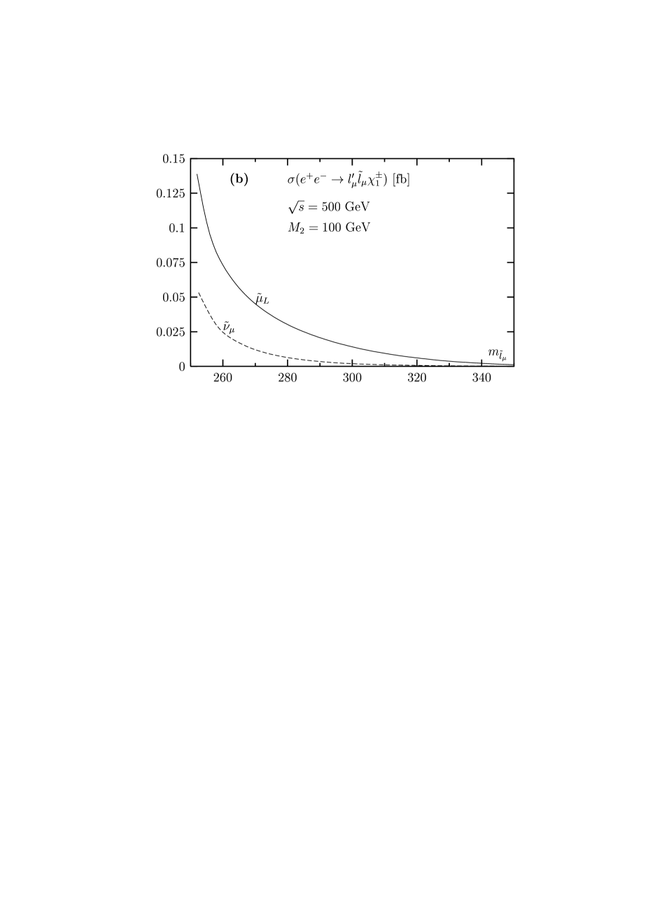
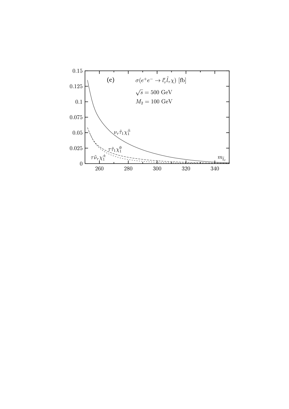
Figure 3: Associated production cross sections for sleptons and gauginos in $e^{+}e^{-}$ collisions for a c.m. energy $\sqrt{s}=500$ GeV as a function of the slepton masses. For the SUSY parameters, we have set $m_{\tilde{\ell}_{L}}=m_{\tilde{\ell}_{R}},M_{2}=100$ GeV, $\mu=500$ GeV and $\tan\beta=30$.

Figure 4: Associated production cross sections for sleptons and gauginos in $e^{+}e^{-}$ collisions for a c.m. energy $\sqrt{s}=1$ TeV as a function of the slepton masses. For the SUSY parameters, we have set $m_{\tilde{\ell}_{L}}=m_{\tilde{\ell}_{R}},M_{2}=100$ GeV, $\mu=500$ GeV and $\tan\beta=30$.

The cross sections for the same associated production processes but for a center of mass energy $\sqrt{s}=1$ TeV are shown in Fig. 4 as a function of the slepton masses for the same set of inputs as in Fig. 3. The production rates are smaller than in the previous case, a consequence of the fact that the dominant contributing channels are the $s$–channel diagrams, which scale like $1/s$ at high–energy. This drop should however be partly compensated by the increase of the luminosity with energy [as expected for the TESLA machine for instance], allowing for a reasonable number of events for slepton masses a few tens of GeV above the kinematical threshold.

Fig. 5 shows the associated production cross sections in the smuon sector in two particular cases for a c.m. energy $\sqrt{s}=500$ GeV. In Fig.5a, the cross sections for $\tilde{\mu}_{L}$ and $\tilde{\nu}_{\mu}$ production in association with the heavier neutral gaugino $\chi_{2}^{0}$ are displayed [again, $\tilde{\mu}_{R}$ does not couple to $\chi_{2}^{0}$ in this case]. Approximately, they are the same and equal to the ones with LSP final states close to the kinematical thresholds, despite the fact that $m_{\chi_{2}^{0}}\simeq 2m_{\chi_{1}^{0}}$. In Fig. 5b, we show the cross section for a fixed slepton mass of $m_{\tilde{\ell}}=275$ GeV and a varying $M_{2}$ parameter. While the variations of $\sigma(e^{+}e^{-}\to\mu\tilde{\mu}_{L}\chi_{1}^{0})$ and $\sigma(e^{+}e^{-}\to\mu\tilde{\mu}_{L}\chi_{2}^{0})$ are mild, the cross section $\sigma(e^{+}e^{-}\to\nu_{\mu}\tilde{\mu}_{L}\chi_{1}^{+})$ drops quickly with increasing $M_{2}$. Therefore, the cross sections for the associated production of smuons with heavier chargino states will be in general smaller than what was shown in Figs. 3 and 4.

Figure 5: Associated production cross sections for sleptons and gauginos in $e^{+}e^{-}$ collisions for a c.m. energy $\sqrt{s}=500$ GeV as a function of the slepton masses with $\chi=\chi_{2}^{0}$ (a) and as a function of the gaugino mass parameter $M_{2}$ with $\chi=\chi^{0}_{1,2}$ (b).

Finally, Fig. 6 shows the production cross sections for the case where the lightest neutralino is higgsino–like in Fig. 6a [with $\mu=100$ GeV and $M_{2}=500$ GeV] or a mixture of higgsino and gaugino states in Fig. 6b [with $M_{2}=\mu=150$ GeV leading to $\chi_{1}^{+}$ masses $m_{\chi_{2}^{\pm}}\sim 2m_{\chi_{1}^{\pm}}\sim 200$ GeV]. As mentioned earlier, the cross sections are extremely small in the higgsino case and the situation should be the same for the production of smuons with $\chi_{2}^{0}$ and $\chi_{1}^{\pm}$, and also for the production of $\tilde{\tau}$’s with higgsinos for not too large values of $\mu$ and $\tan\beta$. However, for the mixed case, the cross sections are only slightly smaller than in the gaugino case. This is due to to the fact that all neutralino and chargino states [which share the gaugino couplings] have to be taken into account, leading to an overall contribution which is not very far from the one for the pure gaugino case.

Figure 6: Associated production cross sections for sleptons and gauginos in $e^{+}e^{-}$ collisions for a c.m. energy $\sqrt{s}=500$ GeV as a function of the slepton masses for the higgsino case (a) and the mixed gaugino–higgsino case (b).

Let us now turn to the case of $\tilde{t}$ and $\tilde{b}$ squarks. The cross sections for the associated production of these squarks with the lightest neutralino and chargino are shown in Fig. 7 for center of mass energies of 500 GeV (a), 1 TeV (b) and 3 TeV (c). In the 500 GeV case where phase space plays an important role due to the heaviness of the top quark, the largest cross section is obtained in the case of $e^{+}e^{-}\to b\tilde{b}_{1}\chi_{1}^{0}$ but it barely reaches the level of 0.03 fb for $m_{\tilde{b}_{1}}\sim 260$ GeV, leading to not much more than 10 events for a luminosity of $\int{\cal L}\sim 500$ fb^-1. It is followed by the cross section for $e^{+}e^{-}\to b\tilde{t}_{1}\chi_{1}^{\pm}$ which is approximately a factor of two smaller. The cross section for $e^{+}e^{-}\to t\tilde{t}_{1}\chi_{1}^{0}$ is one order of magnitude smaller because of the strong suppression by the phase space [since for $m_{\tilde{t}_{1}}\raisebox{-3.69899pt}{~{}\shortstack{$>$ \\ [-0.07cm] $\sim$}}~{}250$ GeV, $m_{t}+m_{\tilde{t}_{1}}+m_{\chi_{1}^{0}}\raisebox{-3.69899pt}{~{}\shortstack{$>$ \\ [-0.07cm] $\sim$}}~{}475$ GeV, i.e. close to $\sqrt{s}=500$ GeV] while the process $e^{+}e^{-}\to t\tilde{b}_{1}\chi_{1}^{\pm}$ is not kinematically accessible at this energy.

At higher energies, Figs. 7b and 7c, the largest cross section is $\sigma(e^{+}e^{-}\to b\tilde{t}_{1}\chi_{1}^{\pm})$, which at $\sqrt{s}=1$ TeV can reach the level of 0.1 fb for a stop mass of a few tens of GeV above the kinematical threshold, followed respectively, by the cross sections $\sigma(e^{+}e^{-}\to t\tilde{t}_{1}\chi_{1}^{0})$, $\sigma(e^{+}e^{-}\to t\tilde{b}_{1}\chi_{1}^{\pm})$ and $\sigma(e^{+}e^{-}\to b\tilde{b}_{1}\chi_{1}^{0})$ which, up to a factor of two, have the same size. This hierarchy of cross sections near the threshold follows from the dominance of final states with stop squarks since the main contribution comes from the $s$–channel production of stops with photon–exchange [because of the larger $Q_{\tilde{t}}$] and by the fact that charged current processes are more favored. At even higher energies, Fig. 7c, the trend is similar to the previous case, but the cross sections are smaller since the contributions of the dominant $s$–channels scale like $1/s$.

Finally, the cross sections for the associated production of third generation squarks with gluinos are shown in Fig. 8. Here, there are two kinematical situations which are relevant for a (genuine) three–body particle final state: $(i)$ if the gluino is heavier than squarks and in this case, it is the only way to produce gluinos in $e^{+}e^{-}$ collisions [except for the loop induced production of gluino pairs [17] for which the cross sections are too small] and $(ii)$ if the gluinos are lighter than squarks, with the latter not being kinematically accessible in pairs in $e^{+}e^{-}$ collisions [otherwise, one can produce squarks which then decay into a quark and a gluino pair, with a branching ratio that is dominant since it is a strong interaction process]. The cross sections for gluino production in association of $\tilde{b}_{1}$ and $\tilde{t}_{1}$ squarks are shown for c.m. energies of 1 TeV (Figs. 8a,8c) and 3 TeV (Figs. 8b,8d) in these two kinematical regimes. In the first situation [gluino heavier than squarks], the production cross sections can reach the level of a fraction of a femtobarn leading to a few tens of events for the expected luminosities, $\int{\cal L}\sim 500$ fb^-1. In the second situation [squarks heavier than gluinos], the cross sections are rather tiny [below 0.01 fb] and higher luminosities are needed to detect these final states.

Figure 7: Associated production cross sections for squarks and electroweak gauginos in $e^{+}e^{-}$ collisions for a c.m. energies of $\sqrt{s}=500$ GeV (a), 1 TeV (b) and 3 TeV (c) as a function of the squark masses. For the SUSY parameters, we have set $m_{\tilde{q}_{L}}=m_{\tilde{q}_{R}},M_{2}=100$ GeV (150 GeV in c), $\mu=500$ GeV and $\tan\beta=30$.

Figure 8: Associated production cross sections for $\tilde{b}_{1}$ and $\tilde{t}_{1}$ squarks and gluinos in $e^{+}e^{-}$ collisions for a c.m. energy $\sqrt{s}=1$ TeV (a,c) and 3 TeV (b,d) as a function of the squark masses. For the SUSY parameters, we have set $M_{2}=350$ GeV (525 GeV) in a-c (b-d), $\mu=500$ GeV and $\tan\beta=30$. The increase of the cross section in (a) for sbottoms for $m_{\tilde{b}_{1}}\sim m_{\tilde{g}}$ is due to the small virtuality of $\tilde{b}_{1}$ in this case. The kink in (b) is due to the heavier $\tilde{b}_{2}$ (exchanged in the $s$–channel digram with a $Z$) becoming close in mass to the gluino. For stops, this is not apparent in the curves because of the large value of $m_{t}$.

4. The cross sections in various approximations

As mentioned in section 2.3 and 3.1, the bulk of the production cross sections for the associated production of sfermions, fermions and electroweak gauginos is due to the contributions of the $s$–channel diagrams, Figs. 1a–1c. In particular, near the kinematical threshold for sfermion pair production, $\sqrt{s}\simeq 2m_{\tilde{f}}$, the contribution of digram (1a) with an almost resonant sfermion is dominant. However, this diagram is not gauge invariant by itself, although in a covariant gauge, the gauge parameter dependence drops out. Furthermore, very close to the kinematical threshold, the zero–width approximation is not valid anymore and one has to include the total decay width of the sfermion in the Breit–Wigner form of the resonant propagator. This is performed by substituting in the sfermion propagator, the squared mass $m_{\tilde{f}}^{2}$ by $m_{\tilde{f}}^{2}-im_{\tilde{f}}\Gamma_{\tilde{f}}$. In fact, near this kinematical threshold, the three–body approximation is not accurate anymore and for a more reliable result one has to consider the four–body process with the production of two off–shell sfermions which then split [or decay if one is above threshold] into fermions and gauginos. Here again, the sole contribution of this double resonant diagram [which, in general, is the only one taken into account in experimental analyses, see Ref. [18] for instance] is not gauge invariant and one should take into account additional diagrams with single resonant states [i.e. with only one intermediate sfermion state or with neutralino or chargino states] [11].

In this section, we will therefore discuss in more details the magnitude of the production cross sections in the various approximations taking as example the associated production of the right–handed smuon, a muon and the LSP, $e^{+}e^{-}\to\mu^{+}\tilde{\mu}_{R}\chi_{1}^{0}$ and the charge conjugate final state $\mu^{-}\tilde{\mu}_{R}^{*}\chi_{1}^{0}$. The total decay width of the right–handed smuon, assuming that the LSP is a pure bino [which implies that $\tilde{\mu}_{R}$ does not couple not only to the heavier charginos and neutralinos which are higgsino–like but also to the gauginos $\chi_{1}^{\pm}$ and $\chi_{2}^{0}$], is identical to the partial decay width into a muon and the LSP which is given by [the couplings given in section 2.2 have been simplified]

$$\Gamma_{\tilde{\mu_{R}}}=\frac{1}{2}\alpha\bigg{(}N^{\prime}_{11}-\frac{s_{W}}{c_{W}}N^{\prime}_{12}\bigg{)}^{2}\,m_{\tilde{\mu}_{R}}\,\bigg{(}1-\frac{m_{\chi_{1}^{0}}^{2}}{m_{\tilde{\mu}_{R}}^{2}}\bigg{)}^{2}$$ (31)

For a 250 GeV $\tilde{\mu}_{R}$, assuming as usual $M_{2}=100$ GeV with $\tan\beta=30$ and $\mu=500$ GeV, the total decay width is $\Gamma_{\tilde{\mu}_{R}}\simeq 1.15$ GeV.

Figure 9: The total cross section for the associated production process $e^{+}e^{-}\to\mu^{-}\tilde{\mu}_{R}^{*}\chi_{1}^{0}$ as a function of the center mass energy in the exact case (solid lines) and in the approximations of the gauge invariant set of diagrams (dashed lines) and the resonant smuon diagram (dotted lines). In panels (a) and (c) the total smuon width is included, while in panel (b) it is set to zero.

In Fig. 9a, we show the cross section for this process as a function of the c.m. energy [varied from 400 to 500 GeV] for $m_{\tilde{\ell}_{L,R}}=250$ GeV and the SUSY parameters given above, retaining $\Gamma_{\tilde{\mu}_{R}}$. While the short–dashed curve shows the contribution of the diagram (1a), the long–dashed curve shows the contribution of the three $s$–channel diagrams (1a), (1b) and (1c), and the full line shows the total contribution including all diagrams.

As one can see, it is a very good approximation [in the present case] to include only the gauge invariant set of contributions (diagrams 1a+1b+1c), since the full line and the long–dashed line are almost overlapping in the entire range of $\sqrt{s}$ values shown in the figure. Far below the kinematical threshold, the contribution of diagram (1a) is rather small, but closer to the threshold where the exchanged smuon is almost on mass–shell, it becomes the dominant one. This is shown in a more explicit way in Fig. 9b, where we zoom on the threshold region. A few GeV near $\sqrt{s}=2m_{\tilde{\mu}_{R}}$, the contribution of the almost–resonant smuon exchange diagram represents 95% of the total cross section. In Fig. 9c, we display the effect including the total width of the smuon in the resonant diagram (1a). As can be seen, the production cross section is slightly lower [by $\sim 5\%$] compared to the zero–width case, Fig. 9b. Therefore, close to the kinematical threshold, one has to include all the $s$–channel diagrams as well as the finite width of the smuon to have a rather accurate estimate of total cross section.

Let us now turn to the discussion of the four–body production process, $e^{+}e^{-}\to\mu^{+}\chi_{1}^{0}\mu^{-}\chi_{1}^{0}$. Taking into account only the gauge invariant set of the double–resonant diagram, $e^{+}e^{-}\to\tilde{\mu}_{R}^{*}\tilde{\mu}_{R}^{*}\to\mu^{+}\chi_{1}^{0}\mu^{-}\chi_{1}^{0}$, plus the single resonant ones with either smuons or gauginos in the intermediate states, 10 Feynman diagrams [the generic form of which can be obtained from the set of diagrams (1a), (1b) and (1c) of Fig. 1, where the smuon splits into a muon and a neutralino] are to be considered. We have calculated the total production cross section, including the finite widths of the smuons, in this approximation using the package CompHEP [16]. This should be a good approximation corresponding to what occurs in the three–body production process. We have compared our results with the ones obtained in Ref. [11] and found perfect agreement.

The four–body cross section, as a function of the c.m. energy, is shown by the solid line of Fig. 10 for the set of inputs chosen previously. It is compared with the cross section for the three–body process below and above threshold [long–dashed lines] and with the cross section of the two–body $e^{+}e^{-}\to\tilde{\mu}_{R}^{+}\tilde{\mu}_{R}^{-}$ production above the threshold with the subsequent decays of the smuons into $\mu\chi_{1}^{0}$ final states [short–dashed lines]. The on–shell smuons are assumed to decay 100% of the time into $\mu\chi_{1}^{0}$ final states. As can be seen, below the kinematical threshold the four–body and the three–body cross section are almost overlapping, which means that it is really a very good approximation to consider in this regime the much simpler three–body production case. Sufficiently above the kinematical threshold, the three–curves also overlap as it should be. A few GeV above the threshold, the three–body and two–body approximations fail badly, and one has to consider the full process with two virtual smuons including their total decay widths in the propagators.

In fact, for a better description of the cross section around the kinematical threshold, which is needed to meet the experimental possibility of measuring the produced smuon mass with a scan near threshold with a precision better than 100 MeV [4], one has not only to use the full four–body production process, $e^{+}e^{-}\to\mu^{+}\mu^{-}\chi_{1}^{0}\chi_{1}^{0}$, including the smuon finite widths, but also to take into account some refinements such as Coulomb re-scattering effects, initial state radiation from the emission of collinear and soft photons and beamstrahlung effects, as discussed in Ref. [11].

Figure 10: Cross section for the two–, three– and four–body processes leading to the final state $\mu^{+}\mu^{-}\chi_{1}^{0}\chi_{1}^{0}$ with intermediate right–handed smuons, around a c.m. energy of 500 GeV. For the SUSY parameters, we have set $M_{2}\simeq 2M_{1}=100$ GeV, $\mu=500$ GeV and $\tan\beta=30$. For the three–body curve, the kink at $\sqrt{s}\simeq 2(m_{\tilde{f}}+\Gamma_{\tilde{f}})$ is due to the “brutal” inclusion of the factor $\frac{1}{2}$ to avoid double counting above threshold; the approximation slightly above threshold is thus rather bad (see text).

5. Conclusion

In this paper, we have analyzed the production at future $e^{+}e^{-}$ colliders of second and third generation sleptons and third generation squarks, in association with their partner leptons and quarks and charginos or neutralinos [and gluinos in the case of squarks], $e^{+}e^{-}\to f\tilde{f}\chi$, in the framework of the MSSM. Analytical expressions for the differential cross sections have been given in the approximation where only the $s$–channel contributing diagrams are taken into account, an approximation which has been shown, a posteriori, to be very good. Taking the example of right–handed smuon production, we have shown that consideration of only the three–body processes is a very good approximation below the kinematical two–sfermion production threshold, but that close to these threshold the full four–body process $e^{+}e^{-}\to f\bar{f}\chi\chi$, including the finite total decay width of the sfermions, have to be considered [11].

We have shown that some of these three–body processes can have sizeable enough production cross sections to allow for the possibility of discovering sfermions with masses a few tens of GeV above the kinematical threshold for sfermion pair production $\sqrt{s}=2m_{\tilde{f}}$ in favorable regions of the SUSY parameter space. This is due to the very high luminosities expected at future linear $e^{+}e^{-}$ colliders, $\int{\cal L}\sim 500$ fb^-1, i.e. three orders of magnitude larger than in the case of LEP2 where the experimental limits on the sfermions masses do not exceed the beam energy. Associated production of squarks and gluinos offers, for some range of sparticle masses, the unique direct access to the gluinos in $e^{+}e^{-}$ collisions, if they are (slightly) heavier than squarks.

The final states discussed in this paper should be clear enough to be easily detected in the clean environment of $e^{+}e^{-}$ colliders. However, for a more precise description, detailed analyses [which are beyond the scope of the present paper] which take into account Standard Model and SUSY backgrounds [as those performed in Ref. [11] in the case of smuon production near threshold] as well as higher order effects and detection efficiencies, have to be performed.

Acknowledgments:

We thank Ayres Freitas and Peter Zerwas for clarifying discussions, Edward Boos and Andrei Semenov for their help in using CompHEP and Yann Mambrini and Margarete Mühlleitner for discussions on Majorana neutralinos. A. Datta is supported by a MNERT fellowship. This work is supported in part by the Euro–GDR Supersymétrie and by the European Union under contract HPRN-CT-2000-00149.

Appendix: the differential cross section

In this appendix, we present the analytical expression of the differential cross section for the associated production of sfermions with charginos or neutralinos

$$e^{+}(p_{1})\;e^{-}(p_{2})\to\tilde{f}_{h}(p_{3})\;\chi_{i}(p_{4})\;\bar{f}^{\prime}(p_{5})$$ (A.1)

where $h=L,R$ is the handedness of the produced sfermion [later on, we will use $h^{\prime}=R,L$ which is the other possible helicity]. To simplify the expressions, we will work in the approximation in which the accompanying fermion in the final state is massless, leading to zero–mixing in the sfermion sector [these expressions are therefore not accurate in the case of associated production with final state top quarks]. Furthermore, we will take into account only the contributions of the gauge invariant set of diagrams Fig 1a, 1b and 1c with $s$–channel exchange of photons and $Z$ bosons which, as shown in the numerical analysis in section 4, is a very good approximation to the full cross section.

The complete spin-averaged matrix element squared for vanishing final state fermion mass and zero–mixing in the scalar sector, is given by

$$|{\cal M}|^{2}=4N_{c}\frac{(4\pi\alpha)^{3}}{s^{2}_{W}}\;\sum_{i\geq j=a,b,c}T_{ij}$$ (A.2)

where $N_{c}$ is the color factor and $\alpha$ is the fine structure constant. The $T_{ij}$ are the amplitudes squared with $i=j=a,b,c$ of the contributions of diagrams $1a,1b$ or $1c$ where the $\gamma$ and $Z$ boson amplitudes have been added, and the interference terms are obtained for $i\neq j=a,b,c$; here the effects of permutations of suffixes are already included in the original terms and hence such permutations are to be left out.

The diagonal terms are given by:

$$T_{aa} = \frac{A_{ih}^{2}}{\{(q-p_{{}_{3}})^{2}-m_{{\tilde{f}_{h}}}^{2}\}^{2}}\left[\frac{Q_{f}^{2}}{s^{2}}+\frac{a_{Z\tilde{f}\tilde{f}}^{2}}{s^{4}_{W}c^{4}_{W}}\frac{(a_{e}^{2}+v_{e}^{2})}{(s-m_{Z}^{2})^{2}}-2\frac{Q_{f}a_{Z\tilde{f}\tilde{f}}v_{e}}{s^{2}_{W}c^{2}_{W}s(s-m_{Z}^{2})}\right]K_{1}$$ (A.3)

$$T_{bb}=\frac{A_{ih}^{2}}{\{(q-p_{{}_{5}})^{2}-m_{f}^{2}\}^{2}} \Biggl{[} \hskip-10.0pt\left\{\frac{Q_{f}^{2}}{s^{2}}+\frac{(a_{e}^{2}+v_{e}^{2})(a_{f}-v_{f})^{2}}{s^{4}_{W}c^{4}_{W}(s-m_{Z}^{2})^{2}}+\frac{2Q_{f}(a_{f}-v_{f})v_{e}}{s^{2}_{W}c^{2}_{W}s(s-m_{Z}^{2})}\right\}K_{2}$$ (A.4)

$$- \frac{2a_{e}(a_{f}-v_{f})}{s^{2}_{W}c^{2}_{W}(s-m_{Z}^{2})}\left\{\frac{v_{e}(a_{f}-v_{f})}{s^{2}_{W}c^{2}_{W}(s-m_{Z}^{2})}+\frac{Q_{f}}{s}\right\}K_{2}^{\prime}\Biggr{]}$$

$$T_{cc} = \frac{Q_{\chi}^{2}}{s^{2}}\sum_{j}\frac{A_{jh}^{2}}{\left\{(q-p_{{}_{4}})^{2}-m_{\chi_{j}}^{2}\right\}^{2}}\left\{(m_{\chi_{j}}^{2}-m_{{\tilde{f}_{h}}}^{2})K_{3}+K_{3}^{\prime}+K_{3}^{\prime\prime}\right\}$$

$$+ \frac{(a_{e}^{2}+v_{e}^{2})}{s^{4}_{W}c^{4}_{W}(s-m_{Z}^{2})^{2}}\sum_{k}\frac{A_{kh}^{2}\left\{(m_{\chi_{k}}^{2}{O_{ik}^{h}}^{2}-m_{{\tilde{f}_{h}}}^{2}{O_{ik}^{h^{\prime}}}^{2})K_{3}+{O_{ik}^{h^{\prime}}}^{2}K_{3}^{\prime}+O_{ik}^{h^{\prime}}O_{ik}^{h}K_{3}^{\prime\prime}\right\}}{\left\{(q-p_{{}_{4}})^{2}-m_{\chi_{k}}^{2}\right\}^{2}}$$

$$+ \frac{2v_{e}Q_{\chi}(-1)^{Q_{\chi}}}{s^{2}_{W}c^{2}_{W}s(s-m_{Z}^{2})}\sum_{j,k}\frac{A_{jh}A_{kh}\left\{(m_{\chi_{k}}^{2}O_{ik}^{h}+m_{{\tilde{f}_{h}}}^{2}O_{ik}^{h^{\prime}})K_{3}+O_{ik}^{h^{\prime}}K_{3}^{\prime}+\frac{1}{2}(O_{ik}^{h^{\prime}}+O_{ik}^{h})K_{3}^{\prime\prime}\right\}}{\left\{(q-p_{{}_{4}})^{2}-m_{\chi_{j}}^{2}\right\}\left\{(q-p_{{}_{4}})^{2}-m_{\chi_{k}}^{2}\right\}}$$

while the non–diagonal terms are given by:

$$T_{ab} = \frac{A_{ih}^{2}}{\left\{(q-p_{{}_{3}})^{2}-m_{{\tilde{f}_{h}}}^{2}\right\}\left\{(q-p_{{}_{5}})^{2}-m_{f}^{2}\right\}}\Biggl{[}-\frac{Q_{f}^{2}}{s^{2}}K_{12}$$ (A.6)

$$+ \frac{1}{s^{2}_{W}c^{2}_{W}(s-m_{Z}^{2})}\Biggl{\{}\left\{\frac{a_{Z\tilde{f}\tilde{f}}(a_{f}-v_{f})(a_{e}^{2}+v_{e}^{2})}{s^{2}_{W}c^{2}_{W}(s-m_{Z}^{2})}-\frac{Q_{f}v_{e}}{s}(a_{f}-v_{f}-a_{Z\tilde{f}\tilde{f}})\right\}K_{12}^{\prime\prime}$$

$$- a_{e}\left\{\frac{2a_{Z\tilde{f}\tilde{f}}(a_{f}-v_{f})v_{e}}{s^{2}_{W}c^{2}_{W}(s-m_{Z}^{2})}-\frac{Q_{f}}{s}(a_{f}-v_{f}-a_{Z\tilde{f}\tilde{f}})\right\}K_{12}^{\prime}\Biggr{\}}\Biggr{]}$$

$$T_{ac} = \frac{1}{(q-p_{{}_{3}})^{2}-m_{{\tilde{f}_{h}}}^{2}}\sum_{j}\frac{A_{jh}^{2}}{(q-p_{{}_{4}})^{2}-m_{\chi_{j}}^{2}}\Biggl{[}\frac{Q_{\chi}}{s}\left\{\frac{Q_{f}}{s}-\frac{a_{Z\tilde{f}\tilde{f}}v_{e}}{s^{2}_{W}c^{2}_{W}(s-m_{Z}^{2})}\right\}(K_{13}$$ (A.7)

$$+\frac{(-1)^{Q_{\chi}}}{s^{2}_{W}c^{2}_{W}(s-m_{Z}^{2})}\left\{\frac{Q_{f}}{s}-\frac{a_{Z\tilde{f}\tilde{f}}(a_{e}^{2}+v_{e}^{2})}{s^{2}_{W}c^{2}_{W}(s-m_{Z}^{2})}\right\}(O_{ij}^{h^{\prime}}K_{13}+O_{ij}^{h}K_{13}^{\prime})\Biggr{]}$$

$$T_{bc} = \frac{1}{(q-p_{{}_{5}})^{2}-m_{f}^{2}}\sum_{j}\frac{A_{jh}^{2}}{(q-p_{{}_{4}})^{2}-m_{\chi_{j}}^{2}}\Biggl{[}\frac{Q_{\chi}}{s}\left\{\frac{Q_{f}}{s}-\frac{(a_{f}-v_{f})v_{e}}{s^{2}_{W}c^{2}_{W}(s-m_{Z}^{2})}\right\}(K_{23}^{a}+K_{23}^{b}$$

$$+ K_{23}^{c^{\prime}})+\frac{(-1)^{Q_{\chi}}}{s^{2}_{W}c^{2}_{W}(s-m_{Z}^{2})}\left\{\frac{(a_{f}-v_{f})(a_{e}^{2}+v_{e}^{2})}{s^{2}_{W}c^{2}_{W}(s-m_{Z}^{2})}+\frac{v_{e}}{s}\right\}\left\{O_{ij}^{h^{\prime}}(K_{23}^{a}+K_{23}^{c^{\prime}})+O_{ij}^{h}K_{23}^{b}\right\}$$

$$+ \frac{a_{e}(a_{f}-v_{f})}{s^{2}_{W}c^{2}_{W}(s-m_{Z}^{2})}\left\{(-1)^{Q_{\chi}}\left\{\frac{2v_{e}}{s^{2}_{W}c^{2}_{W}(s-m_{Z}^{2})}+\frac{1}{s}\right\}(O_{ij}^{h}K_{23}^{d^{\prime}}+O_{ij}^{h^{\prime}}K_{23}^{d^{\prime\prime}})-\frac{Q_{\chi}}{s}K_{23}^{d}\right\}\Biggr{]}$$

The factors $K$, which involve the dependence on the momenta, read:

$$K_{1} = p_{{}_{45}}(4p_{{}_{13}}p_{{}_{23}}-m_{{\tilde{f}_{h}}}^{2}s)$$

$$K_{2} = 4p_{{}_{15}}p_{{}_{25}}p_{{}_{45}}+s\left\{p_{{}_{15}}(p_{{}_{14}}-p_{{}_{45}})+p_{{}_{25}}(p_{{}_{24}}-p_{{}_{45}})\right\}$$

$$K_{2}^{\prime} = p_{{}_{45}}(p_{{}_{15}}-p_{{}_{25}})s$$

$$K_{3} = p_{{}_{14}}p_{{}_{25}}+p_{{}_{15}}p_{{}_{24}}$$

$$K_{3}^{\prime} = (p_{{}_{13}}p_{{}_{24}}+p_{{}_{14}}p_{{}_{23}})p_{{}_{35}}$$

$$K_{3}^{\prime\prime} = m_{\chi_{i}}m_{\chi_{j}}s\;p_{{}_{35}}$$

$$K_{12} = 4(p_{{}_{13}}p_{{}_{25}}+p_{{}_{15}}p_{{}_{23}})p_{{}_{45}}-s\,\left\{(p_{{}_{15}}+p_{{}_{25}})p_{{}_{34}}-(p_{{}_{14}}+p_{{}_{24}})p_{{}_{35}}\right\}$$

$$K_{12}^{\prime} = s\,\left\{(p_{{}_{15}}-p_{{}_{25}})p_{{}_{34}}-(p_{{}_{14}}-p_{{}_{24}})p_{{}_{35}}\right\}$$

$$K_{12}^{\prime\prime} = K_{12}-2p_{{}_{35}}p_{{}_{45}}\,s$$

$$K_{13} = 2\left\{(p_{{}_{13}}p_{{}_{25}}+p_{{}_{15}}p_{{}_{23}})p_{{}_{34}}-(p_{{}_{13}}p_{{}_{24}}+p_{{}_{14}}p_{{}_{23}})p_{{}_{35}}\right\}-(4p_{{}_{13}}p_{{}_{23}}-m_{{\tilde{f}_{h}}}^{2}\,s)p_{{}_{45}}$$

$$K_{13}^{\prime} = m_{\chi_{i}}m_{\chi_{j}}\left\{2(p_{{}_{13}}p_{{}_{25}}+p_{{}_{15}}p_{{}_{23}})-p_{{}_{35}}\,s\right\}$$

$$K_{23}^{a} = 2(p_{{}_{13}}p_{{}_{25}}+p_{{}_{15}}p_{{}_{23}})p_{{}_{45}}$$

$$K_{23}^{b} = m_{\chi_{i}}m_{\chi_{j}}\left\{s(p_{{}_{15}}+p_{{}_{25}})-4p_{{}_{15}}p_{{}_{25}}\right\}$$

$$K_{23}^{c} = \left\{s(p_{{}_{14}}+p_{{}_{24}})+2(p_{{}_{14}}p_{{}_{25}}+p_{{}_{15}}p_{{}_{24}})\right\}p_{{}_{35}}-4p_{{}_{15}}p_{{}_{25}}p_{{}_{34}}$$

$$K_{23}^{c^{\prime}} = K_{23}^{c}-2\,s\,p_{{}_{35}}p_{{}_{45}}$$

$$K_{23}^{d} = 2p_{{}_{25}}(p_{{}_{13}}p_{{}_{45}}-p_{{}_{14}}p_{{}_{35}})+{K_{23}^{d}}^{\prime}+{K_{23}^{d}}^{\prime\prime}$$

$$K_{23}^{d^{\prime}} = s\,m_{\chi_{i}}m_{\chi_{j}}(p_{{}_{15}}-p_{{}_{25}})$$

$$K_{23}^{d^{\prime\prime}} = s(p_{{}_{14}}-p_{{}_{24}})p_{{}_{35}}$$ (A.9)

In the above expressions, $h$ is the suffix for the chirality ($L$ or $R$) of the final state sfermion and $h^{\prime}$ is the other chirality ($R$ or $L$); the latter suffix appears only on the couplings $O_{ij}$. $q=p_{{}_{1}}+p_{{}_{2}}$ is the sum of incoming 4-momenta. We used the notation $2v_{e}=C_{L}^{e}+C_{R}^{e}$ and $2a_{e}=C_{L}^{e}-C_{R}^{e}$ and similarly for $v_{f}$ and $a_{f}$. The $p_{ij}$ correspond to the scalar products $p_{i}\cdot p_{j}$ and $s=q^{2}=(p_{1}+p_{2})^{2}$. All other couplings and parameters are defined in the text.

Note that the antisymmetric part in each of the above terms, proportional to $a_{e}$ are pulled out apart and when, integrated over the full angular domain the corresponding contribution which antisymmetric, vanishes.

The differential cross section is obtained by dividing by the flux and multiplying by the phase space,

$${\rm d}\sigma=\frac{1}{2s}\times\frac{1}{(2\pi)^{5}}\frac{{\rm d}^{3}p_{3}}{2E_{3}}\frac{{\rm d}^{3}p_{4}}{2E_{4}}\frac{{\rm d}^{3}p_{5}}{2E_{5}}\delta^{4}(p_{1}+p_{2}-p_{3}-p_{4}-p_{5})\times|M|^{2}$$ (A.10)

The integral over the phase space, to obtain the total production cross section, is then performed numerically.

References

• [1] S. Abel et al., Report of the “SUGRA” working group for “RUN II at the Tevatron”, hep-ph/0003154; H. Baer, C.H. Chen, M. Drees, F. Paige and X. Tata, Phys. Rev. D58 (1998) 075008 and D59 (1999) 055014.
• [2] CMS Collaboration (S. Abdullin et al.), CMS-NOTE-1998-006, hep–ph/9806366; D. Denegri, W. Majerotto and L. Rurua, CMS-NOTE-1997-094, hep–ph/9711357; I. Hinchliffe et al., Phys. Rev. D55 (1997) 5520.
• [3] E. Accomando, Phys. Rept. 299 (1998) 1; American Linear Collider Working Group (T. Abe et al.), Report SLAC-R-570 and hep-ex/0106057; J. Bagger et al., hep-ex/0007022; H. Murayama and M. Peskin, Ann. Rev. Nucl. Part. Sci. 46 (1996) 533.
• [4] TESLA Technical Design Report, Part I: “Executive Summary”, F. Richard, J.R. Schneider, D. Trines and A. Wagner, TESLA report 2001–23; TESLA TDR, Part III: “Physcis at $e^{+}e^{-}$ Linear Collider” D. Heuer, D. Miller, F. Richard and P.M. Zerwas (eds.) et al., Report DESY–01–011C, hep-ph/0106315.
• [5] For recent analyses, see e.g.: G.A. Blair, W. Porod and P.M. Zerwas, Phys. Rev. D63 (2001) 017703; J.L. Feng and M. Peskin, Phys. Rev. D64 (2001) 115002; S.Y. Choi et al., Eur. Phys. J. C8 (1999) 669 and Eur. Phys. J. C14 (2000) 535; S.Y. Choi et al., hep-ph/0108117; B. Allanach, D. Grellscheid and F. Quevedo hep-ph/0111057.
• [6] For reviews on the MSSM, see: P. Fayet and S. Ferrara, Phys. Rep. 32 (1977) 249; R. Barbieri, Riv. Nuov. Cim. 11 (1988) 1; R. Arnowitt and Pran Nath, Report CTP-TAMU-52-93; M. Drees and S.P. Martin, in “Electroweak Symmetry Breaking and New Physics at the TeV Scale”, eds. T. Barklow et al., World Scientific (1996), hep-ph/9504324; S.P. Martin, hep-ph/9709356; J. Bagger, Lectures at TASI-95, hep-ph/9604232; H.P. Nilles, Phys. Rep. 110 (1984) 1.
• [7] H. E. Haber and G. Kane, Phys. Rep. 117 (1985) 75.
• [8] A.H. Chamseddine, R. Arnowitt and P. Nath, Phys. Rev. Lett. 49 (1982) 970; R. Barbieri, S. Ferrara and C.A Savoy, Phys. Lett. B119 (1982) 343; L. Hall, J. Lykken and S. Weinberg, Phys. Rev. D27 (1983) 2359. For recent reviews see S. Abel et al. in Ref. [1] and A. Djouadi, M. Drees and J.L. Kneur, JHEP 0108 (2001) 055.
• [9] A. Bartl, H. Fraas and W. Majerotto, Z. Phys. C34 (1987) 411; M. Chen, C. Dionisi, M. Martinez and X. Tata, Phys. Rep. 159 (1988) 201; B. de Carlos amd M.A. Diaz, Phys. Lett. B417 (1998) 72.
• [10] K.I. Hikasa and M. Kobayashi, Phys. Rev. D36 (1987) 724; M. Drees and K. Hikasa, Phys. Lett. B252 (1990) 127;
• [11] A. Freitas, D.J. Miller and P.M. Zerwas, Eur. Phys. J. C21 (2001) 361.
• [12] M. Drees and O. Eboli, Eur. Phys. J. C10 (1999) 337.
• [13] A. Datta, A. Djouadi and M. Mühlleitner, in preparation.
• [14] J.F. Gunion and H.E. Haber, Nucl. Phys. B272 (1986) 1 and erratum hep-ph/9301205.
• [15] For a summary on the experimental limits on the mass of the Higgs and SUSY particles, see F. Gianotti, talk given at the EPS–HEP–2001, 12–18 July, Budapest.
• [16] A. Pukhov, E. Boos, M. Dubinin, V. Edneral, V. Ilyin, D. Kovalenko, A. Kryukov, V. Savrin, S. Shichanin, and A. Semenov, “CompHEP - a package for evaluation of Feynman diagrams and integration over multi-particle phase space. User’s manual for version 33”, Preprint INP MSU 98-41/542, hep-ph/9908288.
• [17] P. Nelson and P. Osland, Phys. Lett. B115 (1982) 407; G.L. Kane and W.B. Rolnick, Nucl. Phys. B217 (1983) 117; B.A. Campbell, J.A. Scott and M.K. Sundaresan, Phys. Lett. B126 (1993) 376; B. Kileng and P. Osland, Z. Phys. C66 (1995) 503; A. Djouadi and M. Drees, Phys. Rev. D51 (1995) 4997.
• [18] G. Blair and H.U. Martyn, hep–ph/9910416.