Photon splitting in atomic fields

Abstract

Photon splitting due to vacuum polarization in the electric field of an atom is considered. We survey different theoretical approaches to the description of this nonlinear QED process and several attempts of its experimental observation. We present the results of the lowest-order perturbation theory as well as those obtained within the quasiclassical approximation being exact in the external field strength. The experiment where photon splitting was really observed for the first time is discussed in details. The results of this experiment are compared with recent theoretical estimations.

To the memory of our
friend and colleague
Guram Kezerashvili

1. Introduction

Virtual creation and annihilation of electron-positron pairs is known to induce a self-action of an electromagnetic field, which results in such effects as coherent photon scattering and photon splitting in an external field, and photon-photon scattering. Among these processes the latter was the first one subjected to the exhaustive theoretical investigation [1] (see also [2] and references therein). However, this process was never observed experimentally. At present, coherent photon scattering in the electric field of atoms (Delbrück scattering) is investigated in detail both theoretically and experimentally [3, 4, 5]. The amplitudes and cross sections of this process were calculated in the lowest order in $Z\alpha$ (Born approximation) for arbitrary photon energy $\omega$ and exactly in this parameter for $\omega\gg m$, $Z|e|$ is the nucleus charge, $\alpha=\,e^{2}/4\pi\,=1/137$ is the fine-structure constant, $e$ and $m$ are the electron charge and mass, $\hbar=c=1$. It turned out that higher orders of perturbation theory with respect to $Z\alpha$ (Coulomb corrections) play an important role and drastically modify the cross section of Delbrück scattering on heavy atoms at high photon energy. The experience gained at the investigation of Delbrück scattering was extremely useful for the study of photon splitting. In particular, the importance of the Coulomb corrections in the latter was recognized.

In the process of photon splitting, the initial photon turns in the electric field of an atom into two photons sharing its energy $\omega_{1}$. For a long time, the amplitude of this process was known only in the Born approximation [6, 2]. For $\omega_{1}\ll m$, the asymptotic form of the Born amplitude was derived earlier in [7, 8]. First successful estimate of the total cross section of high-energy ($\omega_{1}\gg m$) photon splitting was made in [9]. More accurate results were obtained in [10] within the same approach for the total as well as for the partly integrated cross sections. The detailed numerical investigation based on the results of [6, 2] was performed in [11, 12].

Recently, an essential progress in understanding of photon splitting phenomenon was achieved due to the use of the quasiclassical approach. In papers [13, 14, 15] various differential cross sections of high-energy photon splitting have been calculated exactly in the parameter $Z\alpha$. Similar to the case of Delbrück scattering, the exact cross section turns out to be noticeably smaller than that obtained in the Born approximation. So, the detailed theoretical and experimental investigation of photon splitting provides a new sensitive test of QED when the effect of higher-order terms of the perturbation theory with respect to the external field is very important.

The observation of photon splitting is extremely hard problem due to severe background conditions. The significance of various competing processes depends on photon energy. For instance, at $\omega_{1}\leq m$ the dominant background process is double Compton scattering on atomic electrons. The search for photon splitting in this energy region was performed in two experiments [16, 17]. As pointed out in [16, 17], the results of both experiments do not agree with the theoretical estimates. Nevertheless, the authors of [16] argue that their results strongly indicate the existence of photon splitting. The energy region $\omega_{1}\gg m$ is more favorable for the observation of the phenomenon, though the background is still rather severe. Using the advantage of the intense source of tagged photons, the first successful observation of photon splitting in the energy region $120$ MeV$\leq\omega_{1}\leq 450$ MeV has been performed recently, and the preliminary results are published in [18], [19]. Here we present the new data analysis for this experiment [20]. The results obtained confirm the existence of photon splitting phenomenon. They also make possible the quantitative comparison with the theoretical predictions. Moreover, the attained experimental accuracy allows one to distinguish between the theoretical predictions obtained with or without accounting for the Coulomb corrections. It turns out that the Coulomb corrections essentially improve the agreement between the theory and the experiment.

2. General discussion

Let a photon with 4-momentum $k_{1}$ ($k_{1}^{0}=\omega_{1}=|\bm{k}_{1}|$) and polarization vector $\bm{e}_{1}$ turns in the electric field of an atom into two photons with 4-momenta $k_{2,3}$ ($k_{2,3}^{0}=\omega_{2,3}=|\bm{k}_{2,3}|$) and polarization vectors $\bm{e}_{2,3}$. We assume that the momentum transferred to a nucleus is small as compared to the mass of the nucleus. This condition allows us to neglect the recoil effects and consider an atom as a source of a time-independent electric field. Then, the final photons share the energy of the initial quantum: $\omega_{1}=\omega_{2}+\omega_{3}$. Later we will see that for arbitrary photon energy the main contribution to the total cross section comes from recoil momenta smaller than several tenth of electron mass. Therefore, the approximation of an external field is valid everywhere except the kinematic region where the differential cross section of the process is negligibly small.

The most convenient way to take into consideration an external electromagnetic field in quantum electrodynamics is to use the Furry representation. In this approach the amplitude of a process is described by a set of Feynman diagrams where the electron lines correspond to the Green functions of the Dirac equation in the field. As a result, we obtain the amplitude in the form of series in the parameter $\alpha$, where the coefficients are exact in the external field strength.

Here we consider the amplitude $M$ of photon splitting only in the lowest order in $\alpha$ which is given by the Feynman diagrams shown in Fig. 1.

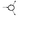
Figure 1: Feynman diagrams for the photon splitting amplitude in the Furry representation. Thick lines denote the electron propagator in an external field

The corresponding analytical expression for $M$ reads

$$M={i}{e^{3}}\int\frac{d\varepsilon}{2\pi}\int d\bm{r}_{1}\,d\bm{r}_{2}\,d\bm{r}_{3}\exp[i(\bm{k}_{1}\cdot\bm{r}_{1}-\bm{k}_{2}\cdot\bm{r}_{2}-\bm{k}_{3}\cdot\bm{r}_{3})]$$ (2..1)

$$\times\mbox{Tr}[\hat{e}_{1}G(\bm{r}_{1},\bm{r}_{2}|\varepsilon-\omega_{2})\hat{e}_{2}^{*}G(\bm{r}_{2},\bm{r}_{3}|\varepsilon)\hat{e}_{3}^{*}G(\bm{r}_{3},\bm{r}_{1}|\varepsilon+\omega_{3})]+(k_{2}^{\mu}\leftrightarrow k_{3}^{\mu},\bm{e}_{2}\leftrightarrow\bm{e}_{3})\,.$$

Here $\hat{e}=e^{\mu}\gamma_{\mu}=-\bm{e}{\bm{\gamma}}$, $\gamma^{\mu}$ being the Dirac matrices, $G(\bm{r}_{1},\bm{r}_{2}|\varepsilon)$ is the Green function of the Dirac equation in the external electric field:

$$G(\bm{r}_{1},\bm{r}_{2}|\varepsilon)=\langle\bm{r}_{1}|[\hat{\mathcal{P}}-m+i0]^{-1}|\bm{r}_{2}\rangle\,,\quad\hat{\mathcal{P}}=\gamma^{0}(\varepsilon-U(\bm{r}))-\bm{\gamma}\cdot\bm{p}\,,$$ (2..2)

$\bm{p}=-i\bm{\nabla}$, $U(\bm{r})$ is the potential energy of an electron. Note that, according to the Furry theorem, the amplitude (2..1) is an odd function of the external field strength (of the parameter $Z\alpha$ for a Coulomb field).

The differential cross section of photon splitting has the form

$$d\sigma=\frac{1}{2^{8}\pi^{5}}|M|^{2}\,\omega_{1}^{2}\,x(1-x)\,dx\,d\Omega_{2}\,d\Omega_{3}\,,$$ (2..3)

where $x=\omega_{2}/\omega_{1}$ (so that $\omega_{3}=\omega_{1}(1-x)$), and $\Omega_{2,3}$ are solid angles of $\bm{k}_{2,3}$. It is convenient to perform the calculations in terms of the helicity amplitudes $M_{\lambda_{1}\lambda_{2}\lambda_{3}}(\bm{k}_{1},\bm{k}_{2},\bm{k}_{3})$, with $\lambda_{i}=\pm 1$. In this case the polarization vectors satisfy the relations $\bm{e}_{\lambda}\cdot\bm{k}=0$ and $\bm{e}_{\lambda}\times\bm{k}=i\lambda\,\omega\bm{e}_{\lambda}$. In fact, it is sufficient to calculate three amplitudes, e.g., $M_{+++}(\bm{k}_{1},\bm{k}_{2},\bm{k}_{3})$, $M_{++-}(\bm{k}_{1},\bm{k}_{2},\bm{k}_{3})$, and $M_{+--}(\bm{k}_{1},\bm{k}_{2},\bm{k}_{3})$. Due to parity conservation and identity of photons, other amplitudes can be obtained by the substitutions (see, e.g. [6]). The cross section $d\sigma_{\lambda_{1}\lambda_{2}\lambda_{3}}$ for circularly polarized photons is given by (2..3) with $M$ being $M_{\lambda_{1}\lambda_{2}\lambda_{3}}$. For unpolarized initial photon the cross section summed up over the polarizations of final photons is given by (2..3) substituting for $|M|^{2}$

$$|M|^{2}\to\frac{1}{2}\sum_{\lambda_{i}}|M_{\lambda_{1}\lambda_{2}\lambda_{3}}|^{2}\,.$$ (2..4)

Below we use the system of coordinates with $z$-axis directed along $\bm{k}_{1}$ so that $a_{z}=\bm{a}\cdot\bm{k}_{1}/\omega_{1}$ and $\bm{a}_{\perp}=\bm{a}-a_{z}\bm{k}_{1}/\omega_{1}$ for an arbitrary vector $\bm{a}$. Then the amplitudes depend on $x=\omega_{2}/\omega_{1}$, polar angles $\theta_{2,3}$ and azimuth angles $\phi_{2,3}$ of the vectors $\bm{k}_{2,3}$. For spherically symmetric potential the quantity $|M_{\lambda_{1}\lambda_{2}\lambda_{3}}|^{2}$ depends on azimuth angles only via $\phi=\phi_{2}-\phi_{3}$. In this case, due to the parity conservation, we have

$$|M_{\lambda_{1}\lambda_{2}\lambda_{3}}(\phi)|^{2}=|M_{\Lambda_{1}\Lambda_{2}\Lambda_{3}}(-\phi)|^{2}\,,$$ (2..5)

where $\Lambda_{i}$ denote the helicity opposite to $\lambda_{i}$. Generally speaking, $|M_{\lambda_{1}\lambda_{2}\lambda_{3}}(\phi)|^{2}$ is not an even function of $\phi$.

Four theoretical approaches, having different ranges of applicability have been used for calculation of the cross section of photon splitting in an atomic field. Three of them use the first-order perturbation theory in the field strength, thereby implying $Z\alpha\ll 1$. They are

• The approach exploiting the Heisenberg-Euler effective Lagrangian, which can be used only for $\omega_{1}\ll m$.

• The Weizsäcker-Williams approximation, valid for $\omega_{1}\gg m$, and providing the logarithmic accuracy for the cross section of the process.

• The calculation of the amplitude exactly with respect to all kinematic parameters of the problem. This approach will be referred below as the Born approximation.

The fourth method is based on the quasiclassical approximation valid for $\omega_{1}\gg m$. In contrast to the approaches itemized, it gives the cross section exact in the parameter $Z\alpha$, and provides a power accuracy in the small parameter $m/\omega_{1}$.

All these approaches will be reviewed below.

3. Low-energy photon splitting

The Heisenber-Euler effective Lagrangian (HEL), derived in [21], describes self-action of an electromagnetic field due to the vacuum polarization when the momenta of quanta are small compared to the electron mass $m$. This Lagrangian depends on two invariants of the electromagnetic field:

$${\mathcal{F}}=\frac{1}{2}(\bm{H}^{2}-\bm{E}^{2})\quad,\quad{\mathcal{G}}=\bm{E}\cdot\bm{H}\,.$$

The lowest order term of the expansion of the HEL with respect to these invariants reads

$${\mathcal{L}}=\frac{e^{4}}{360\pi^{2}m^{4}}\left[(\bm{E}^{2}-\bm{H}^{2})^{2}+7(\bm{E}\cdot\bm{H})^{2}\right]$$ (3..1)

To calculate the photon splitting amplitude, it is necessary to present the electromagnetic field in (3..1) as a sum of a quantized field and the classical electric field of an atom and take the corresponding matrix element. The result obtained accounts for a single Coulomb exchange and holds for $\omega_{1}\ll m$ (and, hence, $\omega_{2,3}\ll m$) because the momentum transfer $\bm{\Delta}=\bm{k}_{2}+\bm{k}_{3}-\bm{k}_{1}$ in this exchange is also small as compared to $m$. We emphasize that it is impossible to calculate the higher order corrections in $Z\alpha$ (Coulomb corrections) to the photon splitting amplitude using the HEL. This is due to the fact that at the multiple Coulomb exchange the typical momenta of individual Coulomb quanta are of the order of $m$ though the sum of these momenta $\bm{\Delta}$ is small.

The calculation of the low-energy photon splitting amplitude with the use of the HEL was performed in [7, 8]. Unfortunately, these papers contain some misprints in the calculations of total cross section as was pointed out in [11], where the photon splitting was investigated numerically using the amplitudes obtained in [6] in the Born approximation.

It follows from (3..1) that the amplitude of the process in an unscreened Coulomb field has the form

$$M_{\lambda_{1}\lambda_{2}\lambda_{3}}=\frac{Ze^{5}\omega_{1}\omega_{2}\omega_{3}}{45\pi^{2}m^{4}\Delta^{2}} \biggl{\{}(\bm{\Delta}\cdot\bm{e}_{1})(\bm{e}_{2}^{*}\cdot\bm{e}_{3}^{*})\left[1+\lambda_{2}\lambda_{3}+\frac{7}{4}\lambda_{1}(\lambda_{2}+\lambda_{3})\right]$$

$$+(\bm{\Delta}\cdot\bm{e}_{2}^{*})(\bm{e}_{1}\cdot\bm{e}_{3}^{*})\left[1-\lambda_{1}\lambda_{3}+\frac{7}{4}\lambda_{2}(\lambda_{1}-\lambda_{3})\right]$$

$$+(\bm{\Delta}\cdot\bm{e}_{3}^{*})(\bm{e}_{1}\cdot\bm{e}_{2}^{*})\left[1-\lambda_{1}\lambda_{2}+\frac{7}{4}\lambda_{3}(\lambda_{1}-\lambda_{2})\right]\biggr{\}}\,.$$

In the case of the electric field of an atom this amplitude should be multiplied by an atomic form factor $[1-F(\Delta^{2})]$ which accounts for screening. This form factor, being the Fourier transform of a charge density (in units of $Z|e|$), vanishes at $\Delta=0$ and tends to unity for $\Delta\to\infty$. As a function of $\Delta$ it has a typical scale of $r_{c}^{-1}=m\alpha z^{1/3}$. These features are illustrated by a simple representation for the form factor suggested in [22]

$$1-F(\Delta^{2})=\Delta^{2}\sum_{i=1}^{3}\,\frac{\alpha_{i}}{\Delta^{2}+\beta_{i}^{2}}\,,$$ (3..3)

where

$$\alpha_{1} = 0.1,\quad\alpha_{2}=0.55,\quad\alpha_{3}=0.35,\quad\beta_{i}=\beta_{0}b_{i},$$ (3..4)

$$b_{1} = 6,\quad b_{2}=1.2,\quad b_{3}=0.3,\quad\beta_{0}=mZ^{1/3}/121.$$

For $\omega r_{c}\ll 1$, the effect of screening leads to the strong suppression of the cross section of photon splitting as compared to the case of unscreened Coulomb field.

The amplitudes (3.) obey the relation $|M_{\lambda_{1}\lambda_{2}\lambda_{3}}|^{2}=|M_{\Lambda_{1}\Lambda_{2}\Lambda_{3}}|^{2}$ ($\Lambda$ denotes the helicity opposite to $\lambda$). Then, as follows from (2..5), the quantity $|M_{\lambda_{1}\lambda_{2}\lambda_{3}}|^{2}$ is an even function of $\phi$.

The angular distribution of the final photons is rather complicated. This is illustrated in Fig. 2, where the cross section $d\sigma/dx\,d\Omega_{2}d\Omega_{3}$ is shown as a function of $\theta_{3}$ at $\theta_{2}=\pi/10$ and $\phi=0,\pi$.

Figure 2: The cross section $d\sigma/dx\,d\Omega_{2}d\Omega_{3}$ in units of $10^{-4}Z^{2}\alpha^{5}{\omega_{1}}^{6}/{m^{8}}=3.09\cdot Z^{2}(\omega_{1}/m)^{6}$ pb as a function of $\theta_{3}$ for $x=0.4$, $\theta_{2}=\pi/10$, and $\phi=0,\pi$ (dashed and solid curves, respectively).

For $\phi=\pi$ there is a double peak with a narrow notch. Such a structure occurs in the range of the momentum transfer $\Delta\ll\omega_{1}$ where $\theta_{2,3}\ll 1$. Then the bottom of the notch is at $\phi=\pi$, $\theta_{3}=\theta_{2}x/(1-x)$, when $\Delta_{\perp}=0$. Note that for $\phi=0$ the differential cross section has a wide deep around $\theta_{3}=\theta_{2}$. In fact, such a suppression of the cross section, when the vectors $\bm{k}_{2}$ and $\bm{k}_{3}$ are almost parallel, persists for any $\bm{k}_{2}$. The cross section $d\sigma/dx\,d\Omega_{2}$ differential with respect to the momentum of one photon is plotted in Fig. 3 for different values of $x$ as a function of $\cos\theta_{2}$. It is seen that the photons with $1-x\ll 1$ ($x\ll 1$) are emitted preferably along $\bm{k}_{1}$ ($-\bm{k}_{1}$). It is also interesting to consider the dependence of the cross section on the azimuth angle $\phi=\phi_{2}-\phi_{3}$, shown in Fig. 4. This cross section is symmetric with respect to the replacement $x\to 1-x$. One can see that for all $x$ the $\phi$-distribution has a minimum at $\phi=0$. The cross section being the function of $|\phi|$ has a maximum that moves from $|\phi|=\pi$ to $|\phi|=2.35$ when $x$ increases from $0$ to $0.5$. The cross sections $d\sigma_{\lambda_{1}\lambda_{2}\lambda_{3}}/dx$ for different helicities as well as $d\sigma/dx$ for unpolarized photons are shown in Fig. 5. Note that $d\sigma_{++-}/dx$ is not symmetric with respect to substitution $x\to 1-x$. Instead, after this substitution $d\sigma_{++-}/dx$ turns into $d\sigma_{+-+}/dx$.

Figure 3: The cross section $d\sigma/dx\,d\Omega_{2}$ in the same units as in Fig. 2 versus $\cos\theta_{2}$ for $x=0.2,0.4,0.6,0.8$ (dotted, dashed, dash-dotted, and solid curves, respectively).

Figure 4: The cross section $d\sigma/dx\,d\phi$ in the same units as in Fig. 2 versus $\phi$ for $x=0.1,0.3,0.5$ (dashed, dotted, and solid curves, respectively).

Figure 5: The cross section $d\sigma/dx$ in the same units as in Fig. 2, for unpolarized photons (solid curve) and for special cases of helicities: $\lambda_{1}\lambda_{2}\lambda_{3}=+--$ (dotted curve),$++-$ (dashed curve), and $+--$ (dash-dotted curve).

Numerical integration gives the following result for the total cross section in the Coulomb field

$$\sigma=\frac{1}{2}\int\limits_{0}^{1}\frac{d\sigma}{dx}dx=7.6\cdot 10^{-5}\frac{Z^{2}\alpha^{5}}{m^{2}}\left(\frac{\omega_{1}}{m}\right)^{6}\,,$$ (3..5)

which coincides with that obtained in [11]. The factor $1/2$ in front of the integral accounts for the identity of photons.

4. Weizsäcker-Williams approximation

The main contribution to the total cross section of photon splitting for $\omega_{1}\gg m$ comes from the region of small angles $\theta_{2,3}\sim m/\omega_{1}$ and can be obtained within the logarithmic accuracy using the Weizsäcker-Williams (WW) approximation. Using this approximation, rather accurate estimate of the total cross section was first made in [9] and later in [7, 8]. The partially integrated cross section as well as the total one were calculated in this approximation in [10]. In the WW approximation the interaction with a Coulomb quantum is replaced by that with a real photon having the 4-momentum $q=(q^{0},-q^{0}\bm{k}_{1}/\omega_{1})$. Then the cross section of photon splitting in WW approximation is expressed via the cross section of photon-photon scattering $d\sigma_{\gamma\gamma}$ as follows

$$d\sigma=\frac{2Z^{2}\alpha}{\pi}\frac{ds}{s}L(s)d\sigma_{\gamma\gamma}\,,\quad L(s)=\int\limits_{\Delta_{min}}^{\Delta_{eff}}\frac{d\Delta}{\Delta}[1-F(\Delta^{2})]^{2}\,,$$ (4..1)

$$s=(k_{1}+q)^{2}=4\omega_{1}q^{0}\,,\quad\Delta_{min}=\frac{s}{\omega_{1}}\,,\quad\Delta_{eff}=\sqrt{s}\,,$$

where $[1-F(\Delta^{2})]$ is the atomic form factor (3..3). The factor in front of $d\sigma_{\gamma\gamma}(s)$ is the spectral distribution of equivalent photons. The photon-photon scattering cross section has the form

$$d\sigma_{\gamma\gamma}=|\tilde{M}|^{2}\delta(k_{1}+q-k_{2}-k_{3})\frac{d\bm{k}_{2}d\bm{k}_{3}}{32\pi^{2}s\,\omega_{2}\omega_{3}}\,,$$ (4..2)

where $\tilde{M}$ is the amplitude of photon-photon scattering [2]. To eliminate the four-dimensional $\delta$-function in the cross section, it is necessary to integrate over the momentum of one of the final photons, and over $q_{0}$ in (4..1). We have $\bm{k}_{2\perp}+\bm{k}_{3\perp}=0$ or $\phi=\pi$ and $\omega_{2}\theta_{2}=\omega_{3}\theta_{3}$ for small polar angles. Then the differential cross section $d\sigma/dxd\bm{k}_{2\perp}$ has the form

$$\frac{d\sigma}{dxd\bm{k}_{2\perp}}=\frac{Z^{2}\alpha{|\tilde{M}|^{2}}L(s)}{8\pi^{3}x(1-x)s^{2}}\,,\quad s=\frac{{k}_{2\perp}^{2}}{x(1-x)}\,.$$ (4..3)

The differential cross section for unpolarized photons is given by (4..3) substituting for $|\tilde{M}|^{2}$

$$|\tilde{M}|^{2} \to \frac{1}{2}[|\tilde{M}_{++++}|^{2}+|\tilde{M}_{++--}|^{2}+|\tilde{M}_{+-+-}|^{2}+|\tilde{M}_{+--+}|^{2}+4|\tilde{M}_{+++-}|^{2}]\,,$$ (4..4)

where $\tilde{M}_{\lambda_{1}\lambda_{q}\lambda_{2}\lambda_{3}}$ are the helicity amplitudes of photon-photon scattering which explicit form is given in Appendix  A.

Integrating (4..3) over all variables we obtain the total cross section of photon splitting which can be represented in the form [10]

$$\sigma = \frac{2Z^{2}\alpha}{\pi}\int\limits_{0}^{\infty}\frac{ds}{s}\sigma_{\gamma\gamma}(s)L(s)\,.$$ (4..5)

Since the cross section $\sigma_{\gamma\gamma}(s)$ falls off for $s\gg m^{2}$, the integral in (4..5) converges at $s\sim m^{2}$. Within the accuracy provided by the WW method we can take the quantity $L(s=m^{2})$ outside the integral. The magnitude of $L(m^{2})$ strongly depends on the ratio of $\Delta_{min}^{-1}=\omega_{1}/m^{2}$ to the radius of screening $r_{c}\sim[m\alpha Z^{1/3}]^{-1}$. In the region $\omega_{1}\geq m^{2}r_{c}$ we have $L(m^{2})=\ln mr_{c}=\ln(Z^{-1/3}/\alpha)$ and $\sigma$ turns out to be independent of $\omega_{1}$. For $m\ll\omega_{1}\leq m^{2}r_{c}$, when the screening may be neglected, we have $L(m^{2})=\ln(\omega_{1}/m)$. As a result, for the total cross section we have

$$\sigma = 0.725\frac{Z^{2}\alpha^{5}}{m^{2}}\times\left\{\begin{array}[]{ll}\ln(\omega_{1}/m)&\quad\mbox{for $m\ll\omega_{1}\leq mZ^{-1/3}/\alpha$}\\ &\\ \ln(Z^{-1/3}/\alpha)&\quad\mbox{for $\omega_{1}\geq mZ^{-1/3}/\alpha$}\end{array}\right.$$ (4..9)

Recall that this result has the logarithmic accuracy. The coefficient $0.725$ in (4..9) is taken from Eq. (4.2) of [11]. Instead of this number, the approximate value $0.753$ was obtained in [10].

The detailed comparison of the results obtained within WW approximation, the Born approximation, and the quasiclassical approximation will be performed below. Here we only note that the accuracy of (4..9) at $\omega_{1}\gg mZ^{-1/3}/\alpha$ is about $12\%$ but for the differential cross section (4..3) this accuracy may be essentially worse.

5. Born approximation

In two previous sections we have considered photon splitting within the first-order perturbation theory in $Z\alpha$ using some additional approximations valid in restricted kinematic regions. The analytical expression for the amplitudes in the Born approximation valid for arbitrary momenta of photons was obtained for the first time in [6] and later confirmed in [2]. The Feynman diagrams corresponding to the amplitude in the Born approximation are shown in Fig. 6.

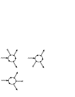
Figure 6: Feynman diagrams for the Born photon splitting amplitude. Wavy lines with crosses denote Coulomb quanta.

For unpolarized photons the result of [6], multiplied by the atomic form factor, reads

$${d\sigma\over dx\,d\Omega_{2}\,d\Omega_{3}}=Z^{2}\alpha^{5}{[1-F(\Delta^{2})]^{2}}\frac{x(1-x)\omega_{1}^{2}}{2\pi^{4}(-\zeta\beta\gamma){\Delta^{4}}}\,\sum_{i=1}^{4}(|x_{i}|^{2}+\eta|y_{i}|^{2})\,,$$ (5..1)

where

$$\zeta = -2k_{2}k_{3}/m^{2}\,,\ \beta=2k_{1}k_{2}/m^{2}\,,\ \gamma=2k_{1}k_{3}/m^{2}\,,\ \eta=4(\bm{k}_{1}\cdot[\bm{k}_{2}\times\bm{k}_{3}])^{2}/m^{6}\,.$$ (5..2)

The quantities $x_{i}$ and $y_{i}$ depend on $\omega_{i}$ and invariants $\zeta$, $\beta$, $\gamma$. Their explicit form being very cumbersome is presented in Appendix  B.

The numerical investigation of various differential cross sections of photon splitting, based on the analytical result of [6], was performed in [11]. The results of [11] are quoted in this section. Shown in Fig. 7 is the dependence of the total Born cross section on $\omega_{1}$ for screened and unscreened Coulomb potentials. The values of this cross section are listed in Table C.2 of Appendix  C for various $Z$ and $\omega_{1}$.

Figure 7: The cross section $\sigma/Z^{2}\mathrm{(nb)}$ plotted as a function of $\omega_{1}$ for a Coulomb potential (solid curve), and the screened potential at $Z=1$ and $Z=92$ (dashed and dotted curves, respectively).

The numerical results for the total cross section at $\omega_{1}\leq 0.1m$, obtained in [11], coincide with (3..5). The analytical fit to the cross section in a Coulomb field, reproducing the cross section in the range $10m\leq\omega_{1}\leq 3000m$ within $0.1\%$, reads

$$\sigma_{unscr}=Z^{2}\left[22.372\ln\frac{\omega_{1}}{m}-47.313+82.536\frac{m}{\omega_{1}}-31.64\left(\frac{m}{\omega}\right)^{2}\right]\,\mathrm{nb}\,.$$ (5..3)

In contrast to the case of a Coulomb field, when the total cross section grows logarithmically with increasing $\omega_{1}$, the photon splitting cross section in the case of a screened Coulomb field is saturated for $\omega_{1}\gg mZ^{-1/3}/\alpha$. This trend is clearly seen in Fig. 7. Note that the difference of the cross sections for screened and Coulomb fields at $\omega_{1}=mZ^{-1/3}/\alpha$ is small (a few percent).

The quasiclassical approach presented in the next Section allows one to obtain the photon splitting cross section for $\omega\gg m$ with a power accuracy in the parameter $m/\omega_{1}$. Therefore, the results obtained within this approximation reproduce for $Z\alpha\ll 1$ two first terms of (5..3). Thus, the accuracy of the quasiclassical approach can be estimated by the relative magnitude of two last terms in (5..3). This accuracy turns out to be better than $1\%$ at $\omega_{1}>70$MeV.

In Fig. 8 the spectrum $\sigma^{-1}d\sigma/dx$ for a Coulomb field is plotted as a function of $x$ for different values of $\omega_{1}$. One can see that the shape of the spectrum changes significantly with increasing photon energy. The detailed data obtained in [11] for spectrum in screened and Coulomb fields are presented in Appendix  C in the Table C.3.

Figure 8: The spectrum $\sigma^{-1}d\sigma/dx$ is plotted for the case of a Coulomb potential as a function of $x$ for $\omega_{1}/m=1,10,100$ (solid, dashed, and dotted curves, respectively).

In order to realize the accuracy of the Born approximation at $Z\alpha\sim 1$ it is necessary to calculate the Coulomb corrections. This issue is elucidated in the next Section.

6. High-energy photon splitting

Small scattering angles of particles provide the applicability of the quasiclassical approach to the description of various high-energy processes in an external field. This approach gives the transparent physical picture of phenomena and essentially simplifies calculations. Recall that the region of small angles $\theta_{2,3}\ll 1$ makes the main contribution to the total cross section of photon splitting for $\omega_{1}\gg m$. That is why we confine ourselves on this kinematic region when considering the process in this Section. Below we quote the results obtained in the quasiclassical approximation in [13, 14, 15]. The technique used in these papers was developed in [23, 24] for the investigation of coherent photon scattering in a Coulomb field.

We choose the origin at the center of a potential and direct the $z$-axis along $\bm{k}_{1}$. Then characteristic values of transverse components of $\bm{r}_{i}$ making the main contribution to the integral in (2..1) at given momentum transfer $\bm{\Delta}=\bm{k}_{2}+\bm{k}_{3}-\bm{k}_{1}$ are of the order of $\rho\sim 1/\Delta$. At small angles the characteristic angular momentum is $l\sim\omega/\Delta\gg 1$, and the quasiclassical approximation can be applied.

It is important that for $\omega\gg m$ the exact in $Z\alpha$ amplitude of photon splitting in the atomic field can be obtained from that calculated for a Coulomb field. For this purpose, we represent the amplitude as a sum of the lowest in $Z\alpha$ term (Born amplitude) and the Coulomb corrections. As explained above, the Born amplitude of the process in the atomic field is a product of that in the Coulomb field and the atomic form factor. In the perturbation theory the Coulomb corrections correspond to the multiple interaction with quanta of an external field. The sum of the momenta of these quanta equals $\bm{\Delta}$. It turns out that even for $\Delta\ll m$ the characteristic magnitude of the momentum of each quantum is not small as compared to $m$. As $m\gg r_{c}^{-1}$ all form factors appearing in the calculation of the Coulomb corrections should be set to unity. Thereby, the Coulomb corrections are the same for the atomic and Coulomb fields.

6.1 Quasiclassical picture of the process

The calculation of the amplitude of photon splitting is essentially simplified by using the Green function $D(\bm{r}_{1},\bm{r}_{2}|\varepsilon)$ of the “squared” Dirac equation:

$$D(\bm{r}_{1},\bm{r}_{2}|\varepsilon)=\langle\bm{r}_{1}|[\hat{\mathcal{P}}^{2}-m^{2}+i0]^{-1}|\bm{r}_{2}\rangle\,.$$ (6..1)

The Green function $G(\bm{r}_{1},\bm{r}_{2}|\varepsilon)$ of the Dirac equation can be obtained from $D(\bm{r}_{1},\bm{r}_{2}|\varepsilon)$ by means of the relation

$$G(\bm{r}_{1},\bm{r}_{2}|\varepsilon)=[\gamma^{0}(\varepsilon-U(\bm{r}_{1}))+i\bm{\gamma}\cdot\bm{\nabla}_{1}+m]D(\bm{r}_{1},\bm{r}_{2}|\varepsilon)\,.$$ (6..2)

As shown in [13, 14], the initial expression for the photon splitting amplitude (2..1) can be presented as a sum of two contributions, containing either three or two Green functions $D(\bm{r}_{1},\bm{r}_{2}|\varepsilon)$: $M=M^{(3)}+M^{(2)}$. The term $M^{(3)}$ is given by

$$M^{(3)} = \frac{i}{2}{e^{3}}\int\frac{d\varepsilon}{2\pi}\int d\bm{r}_{1}d\bm{r}_{2}d\bm{r}_{3}\exp[i(\bm{k}_{1}\cdot\bm{r}_{1}-\bm{k}_{2}\cdot\bm{r}_{2}-\bm{k}_{3}\cdot\bm{r}_{3})]$$ (6..3)

$$\times\mbox{Tr}\{[(-\hat{e}_{1}\hat{k}_{1}-2\bm{e}_{1}\cdot\bm{p})D(\bm{r}_{1},\bm{r}_{2}|\varepsilon-\omega_{2})][(\hat{e}_{2}^{*}\hat{k}_{2}-2\bm{e}_{2}^{*}\cdot\bm{p})D(\bm{r}_{2},\bm{r}_{3}|\varepsilon)]$$

$$\times[(\hat{e}_{3}^{*}\hat{k}_{3}-2\bm{e}_{3}^{*}\cdot\bm{p})D(\bm{r}_{3},\bm{r}_{1}|\varepsilon+\omega_{3})]\}+(k_{2}^{\mu}\leftrightarrow k_{3}^{\mu},\bm{e}_{2}\leftrightarrow\bm{e}_{3}).$$

Here the operator $\bm{p}=-i\mbox{\boldmath${\nabla}$\unboldmath}$ differentiates the Green functions $D$ with respect to their first argument. The term $M^{(2)}$ reads

$$M^{(2)} = i{e^{3}}\int\frac{d\varepsilon}{2\pi}\int d\bm{r}_{1}d\bm{r}_{2}\,\mbox{Tr}\Bigl{\{}\exp[i(\bm{k}_{1}\cdot\bm{r}_{1}-\bm{k}_{2}\cdot\bm{r}_{2}-\bm{k}_{3}\cdot\bm{r}_{2})]$$ (6..4)

$$\times\bm{e}_{2}^{*}\cdot\bm{e}_{3}^{*}[(-\hat{e}_{1}\hat{k}_{1}-2\bm{e}_{1}\cdot\bm{p})D(\bm{r}_{1},\bm{r}_{2}|\varepsilon-\omega_{1})]D(\bm{r}_{2},\bm{r}_{1}|\varepsilon)$$

$$+\Bigl{[}\exp[i(\bm{k}_{1}\cdot\bm{r}_{1}-\bm{k}_{2}\cdot\bm{r}_{2}-\bm{k}_{3}\cdot\bm{r}_{1})]\bm{e}_{1}\cdot\bm{e}_{3}^{*}D(\bm{r}_{1},\bm{r}_{2}|\varepsilon-\omega_{2})$$

$$\times[(\hat{e}_{2}^{*}\hat{k}_{2}-2\bm{e}_{2}^{*}\cdot\bm{p})D(\bm{r}_{2},\bm{r}_{1}|\varepsilon)]+(k_{2}^{\mu}\leftrightarrow k_{3}^{\mu},\bm{e}_{2}\leftrightarrow\bm{e}_{3})\Bigr{]}\Bigr{\}}.$$

Below the Green function $D(\bm{r}_{1},\bm{r}_{2}\,|\varepsilon)$ will be called the “electron Green function” for $\varepsilon>0$ and the “positron Green function” for $\varepsilon<0$. According to [23, 24], for high energies the main contribution to the integrals in (6..3) and (6..4) comes from the region of integration over the variables $z_{i}$ ($z$-coordinates of $\bm{r}_{i}$) in which $z^{\prime}\,<\,z$ for the electron Green function $D(\bm{r},\bm{r}\,^{\prime}|\varepsilon)$ and $z^{\prime}\,>\,z$ for the positron Green function. In terms of non-covariant perturbation theory, this corresponds to the contribution of intermediate states (see Fig. 1) for which the difference between their energy $E_{n}$ and the energy of the initial state $E_{0}=\omega_{1}$ is small as compared to $E_{0}$.

The lifetime of the intermediate state in photon splitting can be estimated with the help of the uncertainty relation as $\tau\sim\omega_{1}/(m^{2}+k_{\perp}^{2})$, where $k_{\perp}=\mbox{max}(|\bm{k}_{2\perp}|,\,|\bm{k}_{3\perp}|)$. The characteristic transverse distance between the virtual particles (transverse size of the loop) can be estimated as $(m^{2}+k_{\perp}^{2})^{-1/2}$, which for $\omega_{1}\gg\mbox{max}(m,k_{\perp})$ is much smaller than the length of the loop $\tau$. The quantity $\rho\sim 1/\Delta$ introduced above can be interpreted as a typical transverse distance between the loop and the origin. In the small-angle approximation ($\theta_{2,3}\ll 1$) we have for $\Delta^{2}$

$${\Delta}^{2}=\bm{\Delta}_{\perp}^{2}+\Delta_{z}^{2}=\,(\bm{k}_{2\perp}+\bm{k}_{3\perp}\,)^{2}+\frac{1}{4}\left(\frac{\bm{k}_{2\perp}\,^{2}}{\omega_{2}}+\frac{\bm{k}_{3\perp}\,^{2}}{\omega_{3}}\right)^{2}\,.$$ (6..5)

It is seen from (6..5) that $\Delta_{\perp}\gg\Delta_{z}$ everywhere except a narrow region where $\Delta_{\perp}\ll k_{\perp}$. As pointed out in [14], the amplitude at $\Delta_{\perp}\sim\Delta_{z}$ can be obtained from that derived for $\Delta_{\perp}\gg\Delta_{z}$ by a simple substitution that will be discussed below. The condition $\Delta_{\perp}\gg\Delta_{z}$ implies that $\rho/\tau\ll 1$ and, therefore, the angles between $\bm{k}_{i}$ and $\bm{r}_{i}$ in (6..3) and (6..4) are either small or close to $\pi$. The additional restrictions on the region, making the main contribution to the amplitude for $\Delta_{\perp}\gg\Delta_{z}$, follow from the explicit form of the quasiclassical Green function. For the term $M^{(3)}$ (6..3) they are

$$z_{1}<\,z_{2},z_{3}\quad,\quad z_{1}<0\quad,\quad\mbox{max}(z_{2},\,z_{3})>\,0\,.$$

Similarly, the main contribution to the term $M^{(2)}$ (6..4) is given by the region $z_{1}<0$ and $z_{2}>0$. All these conditions allow one to depict the main contribution to the amplitude $M^{(3)}$ and $M^{(2)}$ in the form of diagrams, shown in Fig. 9.

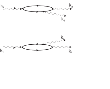
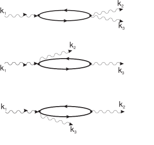
Figure 9: Diagrams corresponding to the terms $M^{(3)}$ (left column) and $M^{(2)}$ (right column).

The explicit form of vertices is obvious from (6..3) and (6..4). The electron Green functions are marked with left-to-right arrows, and positron ones with right-to-left arrows. The arrangement of the diagram vertices is space ordered. With the use of these diagrams one can easily determine the limits of integration over the energy and coordinates. Diagrams in Fig. 9 have a transparent interpretation. For example, the upper left diagram corresponds to the following picture: the photon with momentum $\bm{k}_{1}$ produces, at the point $\bm{r}_{1}$, a pair of virtual particles which is transformed at the point $\bm{r}_{2}$ into a photon with momentum $\bm{k}_{2}$. Between these two events the electron emits a photon with the momentum $\bm{k}_{3}$ at the point $\bm{r}_{3}$.

The quasiclassical Green function $G(\bm{r}_{1},\bm{r}_{2}|\varepsilon)$ of the Dirac equation in a Coulomb potential was first derived in [23] starting from the exact Green function of the Dirac equation [25]. For the case of almost collinear vectors $\bm{r}_{1}$ and $\bm{r}_{2}$ the quasiclassical Green function in arbitrary spherically symmetric decreasing potential was found in [24]. Later in [26] the quasiclassical Green function was obtained in an arbitrary localized potential which generally possesses no spherical symmetry.

As explained above for the calculation of the amplitude of photon splitting in atomic field it is sufficient to know the quasiclassical Green function $D(\bm{r}_{1},\bm{r}_{2}|\varepsilon)$ of the “squared” Dirac equation in a Coulomb field for the case of almost collinear vectors $\bm{r}_{1}$ and $\bm{r}_{2}$. The corresponding expression derived in [13, 14] has the form

$$D(\bm{r}_{1},\bm{r}_{2}|\,\varepsilon) = \,\frac{i\mbox{e}^{i\kappa(r_{1}+r_{2})}}{8\pi^{2}\kappa r_{1}r_{2}}\int d\bm{q}\,\left[1+Z\alpha\frac{\bm{\alpha}\cdot\bm{q}}{q^{2}}\,\right]$$ (6..6)

$$\times\exp{\left[i\frac{q^{2}(r_{1}+r_{2})}{2|\varepsilon|r_{1}r_{2}}+i\bm{q}\cdot(\bm{\vartheta}_{1}+\bm{\vartheta}_{2})\right]}\left(\frac{4\kappa^{2}r_{1}r_{2}}{q^{2}}\right)^{iZ\alpha\eta}$$

for a small angle between vectors $\bm{r}_{1}$ and $-\bm{r}_{2}$. Here $\bm{\alpha}=\gamma^{0}\bm{\gamma}$, $\kappa^{2}=\varepsilon^{2}-m^{2}$, $\eta=\mathrm{sgn}(\varepsilon)$, $\bm{\vartheta}_{1,2}=(\bm{r}_{1,2})_{\perp}/r_{1,2}$, and $\bm{q}$ is a two-dimensional vector lying in $xy$ plane. The direction of $z$ axis is arbitrary provided that $\vartheta_{2,3}\ll 1$. Expression (6..6) contains only elementary functions, and the angles $\bm{\vartheta}_{1}$ and $\bm{\vartheta}_{2}$ appear only in the factor $\exp[i\bm{q}\cdot(\bm{\vartheta}_{1}+\bm{\vartheta}_{2})]$. For a small angle between vectors $\bm{r}_{1}$ and $\bm{r}_{2}$ we have for $D(\bm{r}_{1},\bm{r}_{2}|\,\varepsilon)$

$$D(\bm{r}_{1},\bm{r}_{2}|\,\varepsilon)=-\frac{\e^{i\kappa|\bm{r}_{1}-\bm{r}_{2}|}}{4\pi|\bm{r}_{1}-\bm{r}_{2}|}\,\left(\frac{r_{1}}{r_{2}}\right)^{iZ\alpha\,\eta\,\mathrm{sgn}(r_{1}-r_{2})}\,.$$ (6..7)

One can see that the Green function (6..7) differs from that at vanishing potential only by a phase factor. It is easy to check that after the substitution of the expressions (6..6) and (6..7) for the Green functions to the splitting amplitudes (6..3) and (6..4) all phase factors of the form $r^{\pm iZ\alpha}$ cancel.

6.2 Amplitude of the process

At the calculation of the amplitude it is convenient to eliminate the $z$ component of the polarization vectors $\bm{e}_{i}$ using the relation $\bm{e}_{i}\cdot\bm{k}_{i}=0$ which leads to $e_{iz}=-\bm{e}_{i\perp}\cdot\bm{k}_{i\perp}/k_{iz}$. After that, in the small-angle approximation we can neglect the difference between the polarization vector $\bm{e}_{2\perp}$ ($\bm{e}_{3\perp}$) and that of photon, propagating along the $z$ axis and having the same helicity. As a result, we obtain the amplitudes $M_{\lambda_{1}\lambda_{2}\lambda_{3}}(\bm{k}_{1},\bm{k}_{2},\bm{k}_{3})$ containing only the transverse polarization vectors $\bm{e}$ and $\bm{e}^{*}$ for positive and negative helicities, respectively. Though the Green function $D(\bm{r}_{1},\bm{r}_{2}|\varepsilon)$ (6..6), (6..7) has a simple form, the integration in (6..3) and (6..4) was very sophisticated. The final expressions, obtained in [15], for the helicity amplitudes exact in the parameter $Z\alpha$ have the form

$$M_{+--} = N\!\!\int\!\!d{\bm{x}}\left({\bm{e}\cdot\bm{G}}\right)\!\!\int_{0}^{\omega_{2}}\!\!\frac{d\varepsilon}{A}\kappa_{2}\Biggl{[}-{\bm{e}\cdot\bm{a}}\left(\frac{\varepsilon}{{\bm{e}}^{*}\cdot{\bm{\theta}}_{3}}+\frac{\kappa_{3}}{{\bm{e}}^{*}\cdot{\bm{\theta}}_{23}}\right)$$ (6..10)

$$+m^{2}\omega_{3}\kappa_{2}\left(\frac{\kappa_{3}\,{\bm{e}\cdot\bm{\theta}}_{23}}{\omega_{1}{\mathcal{D}}_{1}{\bm{e}}^{*}\cdot{\bm{\theta}}_{23}}-\frac{\varepsilon\,{\bm{e}\cdot\bm{\theta}}_{3}}{\omega_{2}{\mathcal{D}}_{3}{\bm{e}}^{*}\cdot{\bm{\theta}}_{3}}\right)\Biggr{]}+\left(\begin{array}[]{c}\omega_{2}\leftrightarrow\omega_{3}\\ {\bm{\theta}}_{2}\leftrightarrow{\bm{\theta}}_{3}\end{array}\right),$$

$$M_{+++} = N\!\!\int\!\!d{\bm{x}}\!\!\int_{0}^{\omega_{2}}\frac{d\varepsilon}{2A}\left[\frac{{\bm{e}\cdot\bm{G}}\left(\kappa_{2}^{2}+\kappa_{3}^{2}\right)}{{\bm{e}\cdot\bm{\theta}}_{23}}\left({\bm{e}}^{*}\cdot{\bm{a}}-\frac{m^{2}\omega_{3}\kappa_{2}\,{\bm{e}}^{*}\cdot{\bm{\theta}}_{23}}{\omega_{1}{\mathcal{D}}_{1}}\right)\right.$$ (6..13)

$$+\frac{\omega_{1}\omega_{3}\kappa_{2}G_{1}{\bm{e}}^{*}\cdot\left(\bm{a}+\bm{\theta}_{23}\omega_{2}\kappa_{3}/\omega_{1}\right)}{{\mathcal{D}}_{1}}+\frac{\omega_{3}\kappa_{2}\,{\bm{e}}^{*}\cdot{\bm{G}}}{\omega_{2}{\mathcal{D}}_{3}}\Bigl{[}2\varepsilon\left(\kappa_{2}^{2}+\kappa_{3}^{2}\right)\left({\bm{e}}^{*}\cdot{\bm{\theta}}_{3}\right)\left({\bm{e}\cdot\bm{a}}\right)$$

$$\left.+\varepsilon\omega_{3}A+m^{2}(2\varepsilon\kappa_{2}-\omega_{1}\omega_{2})\Bigr{]}-\frac{\omega_{1}\omega_{3}\kappa_{2}G_{1}\,{\bm{e}}^{*}\cdot{\bm{c}}}{{\mathcal{D}}_{3}}\right]+\left(\begin{array}[]{c}\omega_{2}\leftrightarrow\omega_{3}\\ {\bm{\theta}}_{2}\leftrightarrow{\bm{\theta}}_{3}\end{array}\right),$$

$$M_{++-} = N\int d{\bm{x}\,}\Biggl{\{}\int_{0}^{\omega_{2}}\frac{d\varepsilon}{2A}\left[\frac{\kappa_{2}\omega_{3}\,{\bm{e}}\cdot\bm{G}}{\omega_{1}{\mathcal{D}}_{1}}\Bigl{[}\kappa_{3}\left(\kappa_{2}-\varepsilon\right)A\right.-2\kappa_{3}\left(\kappa_{2}^{2}+\varepsilon^{2}\right)\left({\bm{e}}\cdot\bm{\theta}_{23}\right)\left({\bm{e}}^{*}\cdot{\bm{a}}\right)$$ (6..14)

$$+m^{2}\left(\omega_{1}\omega_{2}-2\kappa_{2}\kappa_{3}\right)\Bigr{]}+\frac{\kappa_{2}\omega_{2}\omega_{3}G_{1}\,{\bm{e}}\cdot\bm{b}}{{\mathcal{D}}_{1}}+\frac{\left(\kappa_{2}^{2}+\varepsilon^{2}\right){\bm{e}}^{*}\cdot{\bm{G}}}{{\bm{e}}^{*}\cdot{\bm{\theta}}_{3}}$$

$$\left.\times\left({\bm{e}}\cdot\bm{a}+\frac{m^{2}\omega_{3}\kappa_{2}\,{\bm{e}}\cdot\bm{\theta}_{3}}{\omega_{2}{\mathcal{D}}_{3}}\right)-\frac{\omega_{2}\omega_{3}\kappa_{2}G_{1}{\bm{e}\cdot}\left({\bm{a}}+\bm{\theta}_{3}\omega_{1}\varepsilon/\omega_{2}\right)}{{\mathcal{D}}_{3}}\right]$$

$$+\int_{-\omega_{3}}^{0}d\varepsilon\frac{\omega_{2}\kappa_{3}}{2B}\left[\frac{{\bm{e}}\cdot\bm{G}}{\omega_{1}{\mathcal{D}}_{1}}\Bigl{[}-\left(\kappa_{2}^{2}+\varepsilon\kappa_{3}\right)B+2\kappa_{3}\left(\kappa_{2}^{2}+\varepsilon^{2}\right)\left({\bm{e}}^{*}\cdot{\bm{\theta}}_{23}\right)\left({\bm{e}}\cdot\bm{b}\right)\right.$$

$$+m^{2}\left(\omega_{1}\omega_{2}-2\kappa_{2}\kappa_{3}\right)\Bigr{]}+\frac{\omega_{2}G_{1}\,{\bm{e}}\cdot\bm{b}}{{\mathcal{D}}_{1}}+\frac{\omega_{2}G_{1}\,{\bm{e}}\cdot\bm{b}}{{\mathcal{D}}_{2}}+\frac{{\bm{e}}\cdot\bm{G}}{\omega_{3}{\mathcal{D}}_{2}}\Bigl{[}-\omega_{2}\kappa_{3}B$$

$$+2\kappa_{3}\left(\kappa_{2}^{2}+\varepsilon^{2}\right)\left({\bm{e}}^{*}\cdot{\bm{\theta}}_{2}\right)\left({\bm{e}}\cdot\bm{b}\right)+m^{2}\left(\omega_{2}\omega_{3}-2\varepsilon\kappa_{3}\right)\Bigr{]}\Biggr{]}\Biggr{\}}\,,$$

where the following notation is used

$$\kappa_{2}=\omega_{2}-\varepsilon\,,\quad\kappa_{3}=\omega_{3}+\varepsilon\,,\quad\bm{\theta}_{23}=\bm{\theta}_{2}-\bm{\theta}_{3}\,,\quad A=m^{2}+{a}^{2}\,,\quad B=m^{2}+{b}^{2}\,,$$

$$\bm{a}=\bm{x}_{-}+\kappa_{2}\bm{\theta}_{2}\,,\quad\bm{b}=\bm{x}_{+}-\kappa_{3}\bm{\theta}_{3}\,,\quad\bm{c}=\bm{x}_{+}-\varepsilon\bm{\theta}_{23}\,,\quad\bm{x}_{\pm}=\bm{x}\pm\bm{\Delta}_{\perp}/2\,,$$

$$N={8e^{3}Z\alpha}[\pi^{2}\Delta^{2}\omega_{1}\omega_{2}\omega_{3}]^{-1}\,,\quad\omega_{1}^{2}{\mathcal{D}}_{1}=\left(\kappa_{2}\bm{x}_{+}+\kappa_{3}\bm{x}_{-}\right)^{2}-\omega_{2}\omega_{3}\kappa_{2}\kappa_{3}{\theta}_{23}^{2}-i0\,,$$

$$\omega_{3}^{2}{\mathcal{D}}_{2}=\left(\varepsilon\bm{x}_{+}-\kappa_{3}\bm{x}_{-}\right)^{2}-\omega_{1}\omega_{2}\kappa_{3}\varepsilon{\theta}_{2}^{2}\,,\quad\omega_{2}^{2}{\mathcal{D}}_{3}=\left(\kappa_{2}\bm{x}_{+}+\varepsilon\bm{x}_{-}\right)^{2}+\omega_{1}\omega_{3}\kappa_{2}\varepsilon{\theta}_{3}^{2}\,.$$

The functions $\bm{G}$ and $G_{1}$ are

$${\bm{G}} = \frac{\pi(1+\xi)}{\sinh(\pi Z\alpha)}\mathrm{Im}\left\{\left[\frac{\bm{x}_{+}}{c_{+}}\left({c_{+}\over c_{-}}\right)^{iZ\alpha}\!\!\!-\frac{\bm{x}_{-}}{c_{-}}\left({c_{-}\over c_{+}}\right)^{iZ\alpha}\right]P_{iZ\alpha}^{\prime}(\xi)\right\}\,,$$

$$G_{1} = \frac{\pi(1+\xi)}{\sinh(\pi Z\alpha)}\mathrm{Im}\left\{\left[\frac{c_{+}-2m^{2}}{2c_{+}}\left({c_{+}\over c_{-}}\right)^{iZ\alpha}\!\!\!-\frac{c_{-}-2m^{2}}{2c_{-}}\left({c_{-}\over c_{+}}\right)^{iZ\alpha}\right]P_{iZ\alpha}^{\prime}(\xi)\right\}\,,$$ (6..15)

where $c_{\pm}=m^{2}+{x}_{\pm}^{2}$, $\,\xi=2m^{2}{\Delta}_{\perp}^{2}/(c_{+}c_{-})-1$, and $P_{iZ\alpha}^{\prime}(\xi)\,=\,dP_{iZ\alpha}(\xi)/d\xi$ is the derivative of the Legendre function. The amplitudes with other helicities can be obtained from (6..10) using the following relations

$$M_{+-+}(\bm{k}_{1},\bm{k}_{2},\bm{k}_{3}) = M_{++-}(\bm{k}_{1},\bm{k}_{3},\bm{k}_{2}),$$

$$M_{-\lambda_{2}\lambda_{3}}(\bm{k}_{1},\bm{k}_{2},\bm{k}_{3}) = M_{+\Lambda_{2}\Lambda_{3}}(\bm{k}_{1},\bm{k}_{2},\bm{k}_{3})\,(\bm{e}\leftrightarrow\bm{e}^{*}),$$ (6..16)

where $\Lambda$ denotes the helicity opposite to $\lambda$.

Since the functions $\bm{G}$ and $G_{1}$ are independent of the energy $\varepsilon$, the integrands in (6..10) are rational functions of $\varepsilon$, in which all the denominators are quadratic forms of this variable. Therefore, the integrals over $\varepsilon$ can be expressed via elementary functions. Resulting formulae being rather cumbersome are not presented here explicitly. Performing the integration over $\varepsilon$ in (6..10), one obtains a twofold integral over $\bm{x}$ for the amplitudes of photon splitting. It has been checked numerically that in the limit $Z\alpha\rightarrow 0$ our results (6..10) agree with those, obtained in [11] in the Born approximation.

Let us comment on the appearance of the total momentum transfer squared $\Delta^{2}$ (see (6..5)) in the coefficient $N$ in (6..10). The amplitudes (6..10) were derived at the assumption $\Delta_{\perp}\gg\Delta_{z}$ when there is no difference between $\Delta^{2}$ and $\Delta_{\perp}^{2}$. Nevertheless, if we retain the term $\Delta_{z}^{2}$ in $\Delta^{2}$ in the coefficient $N$, the formulas (6..10) become valid also for $\Delta_{\perp}\sim\Delta_{z}$. This can be explained as follows. In the region $\Delta_{\perp}\sim\Delta_{z}$ the Born amplitude prevails over the Coulomb corrections (cf. (Appendix  D) and (D.5)). On the other hand, in the small-angle approximation it contains the momentum transfer in the form $\bm{\Delta}_{\perp}/\Delta^{2}$, where $\Delta$ is just the total momentum transfer.

For $\omega_{2}\theta_{2},\,\omega_{3}\theta_{3}\gg m$ we can neglect the electron mass in the expressions (6..10). In this case (zero mass limit) the amplitudes are simplified, which allows us to perform the further analytical investigation of the process (see Appendix  D).

6.3 Cross section

In the small-angle approximation ($\theta_{2,3}\ll 1$) the cross section (2..3) can be represented in the form

$$d\sigma=|M|^{2}\,\frac{dx\,d\bm{k}_{2\perp}\,d\bm{k}_{3\perp}\,}{2^{8}\pi^{5}\omega_{1}^{2}x(1-x)}\,.$$ (6..17)

In this subsection a screened Coulomb potential is used in the numerical calculations. As was explained above, to take screening into account, the Born part of the amplitude should be multiplied by an atomic form factor, e.g. (3..3). To illustrate a magnitude of the Coulomb corrections, the exact and Born differential cross sections for unpolarized photons $d\sigma/dxd\bm{k}_{2\perp}d\bm{k}_{3\perp}$ are plotted in Fig. 10 as a function of $k_{2\perp}/m$ for ${k}_{3\perp}=2m$, $x=0.1$, $\omega_{1}=1$GeV and the azimuth angle (the angle between the vectors $\bm{k}_{2\perp}$ and $\bm{k}_{3\perp}$) $\phi=0$ and $\pi$. The value $Z=83$ (bismuth) was chosen since bismuth atoms determine the cross section of photon splitting in the experiment [18].

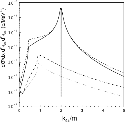
Figure 10: Differential cross section $d\sigma/dxd\bm{k}_{2\perp}d\bm{k}_{3\perp}$ vs ${k}_{2\perp}/m$ in a screened Coulomb potential for different azimuth angle $\phi$ between vectors $\bm{k}_{2\perp}$ and $\bm{k}_{3\perp}$; $Z=83$, $x=0.1$, $\omega_{1}=1$GeV, $k_{3\perp}=2m$. The dashed curve (Born approximation) and the solid curve (exact cross section) correspond to $\phi=\pi$. The dash-dotted curve (Born approximation) and the dotted curve (exact cross section) correspond to $\phi=0$.

A wide peak for azimuth angle $\phi=\pi$ is due to small momentum transfer $\Delta$. There is a narrow notch (c.f. Fig. 2) in the middle of this peak ( at $k_{2\perp}/m=2$ ) where the condition $\bm{\Delta}_{\perp}=\bm{k}_{2\perp}+\bm{k}_{3\perp}=0$ is fulfilled. Such a structure was discussed first in [12]. The width of the notch is about $\mathrm{max}(\Delta_{z}/m,\beta_{0}/m)$. Recall that $\Delta_{z}$ is the longitudinal component of the momentum transfer defined by (6..5), and $\beta_{0}=mZ^{1/3}/121$ (3..3) characterizes the effect of screening. In our example $\beta_{0}$ is larger than $\Delta_{z}$ , so the width of the notch is roughly $\beta_{0}/m=3.6\times 10^{-2}$. Let us note that for $\omega_{1}\gg m$ the differential cross section, expressed in terms of $\bm{k}_{2\perp}$, $\bm{k}_{3\perp}$, $x$, and $\omega_{1}$, depends on $\omega_{1}$ only via $\Delta_{z}$. Due to this fact, the differential cross section is independent of $\omega_{1}$ in the region where we can neglect $\Delta_{z}$, i.e. outside the notch vicinity. For small $\Delta$ as compared to $k_{\perp}$ the Born amplitude, which is proportional to $1/\Delta$, is much larger than the Coulomb corrections. That is why the exact and Born cross sections coincide within the peak region. Outside this region the Coulomb corrections essentially modify the cross section. The points of discontinuous slope of the curves in Fig. 10 are related to the threshold conditions for the production of real electron-positron pair by two photons with the momenta $\bm{k}_{2}$ and $\bm{k}_{3}$:

$$(k_{2}+k_{3})^{2}=\omega_{2}\omega_{3}\theta_{23}^{2}=4m^{2}\ .$$ (6..18)

It is worth noting that the cross section $d\sigma_{\lambda_{1}\lambda_{2}\lambda_{3}}/dx\,d\Omega_{2}d\Omega_{3}$ for definite helicities of photons is not an even function of the azimuth angle $\phi$. Instead, due to the parity conservation the following relation holds

$$\frac{d\sigma_{\lambda_{1}\lambda_{2}\lambda_{3}}}{dx\,d\Omega_{2}d\Omega_{3}}(\phi)=\frac{d\sigma_{\Lambda_{1}\Lambda_{2}\Lambda_{3}}}{dx\,d\Omega_{2}d\Omega_{3}}(-\phi)$$ (6..19)

As an illustration of the azimuth asymmetry of the cross section, the dependence of $S_{+}$ and $\xi=2(S_{+}-S_{-})/(S_{+}+S_{-})$ on the azimuth angle $\phi$ is shown in Fig. 11, where $S_{\pm}=\sum_{\lambda_{2}\lambda_{3}}d\sigma_{\pm\lambda_{2}\lambda_{3}}/dx\,d\Omega_{2}d\Omega_{3}$ are the differential cross sections for positive ($S_{+}$) and negative ($S_{-}$) helicities of the initial photon. Again, the exact in $Z\alpha$ cross section (solid curve in Fig. 11$a$) is much smaller than the cross section obtained in the Born approximation (dashed curve ibid). The magnitude of azimuth asymmetry (Fig. 11$b$) reaches tens of percent. For the parameters used in our example the effect of screening is not essential.

Figure 11: The dependence of $S_{+}$ ($a$) and $\xi=2(S_{+}-S_{-})/(S_{+}+S_{-})$ ($b$) on the azimuth angle $\phi$ at $Z=83$, $\omega_{1}=1$GeV, $x=0.3$, $\theta_{2}=0.014$, and $\theta_{3}=0.02$. Here $S_{\pm}=\sum_{\lambda_{2}\lambda_{3}}d\sigma_{\pm\lambda_{2}\lambda_{3}}/dx\,d\Omega_{2}d\Omega_{3}$ are the differential cross sections for positive ($S_{+}$) and negative ($S_{-}$) helicities of the initial photon. Solid curves represent the exact in $Z\alpha$ results, dashed curves are obtained in the Born approximation.

In Fig. 12 the differential cross section $m^{2}\sigma_{0}^{-1}d\sigma/dx\,d\bm{k}_{2\perp}$ is shown depending on $k_{2\perp}/m$ for a screened Coulomb potential at $\omega_{1}/m=1000$, $Z=83$, and different $x$,

$$\sigma_{0}=\frac{\alpha^{3}(Z\alpha)^{2}}{4\pi^{2}m^{2}}=0.782\cdot 10^{-9}\,Z^{2}\mbox{ b}\ .$$

Figure 12: $m^{2}\sigma_{0}^{-1}d\sigma/dxd\bm{k}_{2\perp}$ vs $k_{2\perp}/m$ for a screened Coulomb potential, $\omega_{1}/m=1000$, $Z=83$, $\sigma_{0}=\alpha^{3}(Z\alpha)^{2}/(4\pi^{2}m^{2})=0.782\cdot 10^{-9}\,Z^{2}\mathrm{b}$, $x=0.2$ ($a$), $0.5$ ($b$), and $0.8$ ($c$). The dashed curves correspond to the Born approximation, the solid curves give the exact result, and the dotted curves show the results of the WW approximation.

Solid curves represent the exact cross sections, the dashed curves give the Born results, and the dotted curves correspond to the WW approximation (4..3). The cross section exhibits a thresholdlike behavior in the vicinity of the point $k_{2\perp}=k_{th}=2\sqrt{x(1-x)}m$, where both conditions $\bm{\Delta}_{\perp}=\bm{k}_{2\perp}+\bm{k}_{3\perp}=0$ and (6..18) hold. Under these conditions the peak in the cross section $d\sigma/dxd\bm{k}_{2\perp}d\bm{k}_{3\perp}$ seats on the boundary of the kinematic region in which the production of a real electron-positron pair by two photons with the momenta $\bm{k}_{2}$ and $\bm{k}_{3}$ is possible. The cross section $d\sigma/dx\,d\bm{k}_{2\perp}$ drops rapidly for $k_{2\perp}\gg m$ ($\propto 1/k_{2\perp}^{4}$). As seen in Fig. 12, the Coulomb corrections to the cross section integrated over $\bm{k}_{3\perp}$ noticeably diminish the magnitude of the cross section. Above the threshold ($k_{2\perp}>k_{th}$) the Coulomb corrections reach tens of percent while below the threshold the exact cross section is several times smaller than the Born one. It can be explained as follows. Above the threshold the main contribution to the cross section $d\sigma/dx\,d\bm{k}_{2\perp}$ is given by the integration region with respect to $\bm{k}_{3\perp}$ where $\mbox{max}(\bm{k}_{2\perp}^{2}/\omega_{1},\beta_{0})\ll\Delta\ll k_{2\perp}$. As a result, the Born cross section is logarithmically amplified as compared to the Coulomb corrections. Far below the threshold where $k_{2\perp}\ll k_{th}$, the region $\Delta\ll k_{2\perp}$ does not contribute to the cross section $d\sigma/dx\,d\bm{k}_{2\perp}$ since in this region $k_{3\perp}\approx k_{2\perp}\ll m$, and the amplitude is suppressed as a power of $k_{2\perp}^{2}/m^{2}$. Therefore, below the threshold the main contribution to the cross section is given by the region $k_{3\perp}\sim m$, where the amplitude, exact in $Z\alpha$, drastically differs from the Born one. Due to the same reason below the threshold the cross section in the WW approximation (dotted curves) differs essentially from the Born result because the former comes from the region $\Delta\ll k_{2\perp}$. As follows from (Appendix  A), for $k_{\perp}\ll m$ the amplitudes entering the cross section (4..3) are suppressed as $k_{\perp}^{4}/m^{4}$. One can see from Fig. 12 that in accordance with the expression for $k_{th}$ the position of the peak is the same for $x=0.2$ and $x=0.8$. Nevertheless, the magnitude of these two cross sections are significantly different, especially below the threshold. However, as expected and verified numerically, the cross section $d\sigma/dx$ at $x=0.2$ coincide with that at $x=0.8$.

Let us consider now the magnitude of the Coulomb corrections to the cross section $d\sigma/dx$ integrated over the transverse momenta of both final photons. The main contribution to this cross section is given by the region where ${k}_{2\perp},\,{k}_{3\perp}\sim m$. The Born contribution to $d\sigma/dx$ contains large logarithm resulting from the integration over small momentum transfer region $\mbox{max}(\beta_{0},m^{2}/\omega_{1})\ll\Delta\ll m$. For $\beta_{0}\gg m^{2}/\omega_{1}$, the cross section $d\sigma/dx$ is independent of $\omega_{1}$, while for $\beta_{0}\ll m^{2}/\omega_{1}$ it grows slowly (as $\ln(\omega_{1}/m)$) when $\omega_{1}$ increases. Since the Coulomb corrections to $d\sigma/dx$ are determined by the region of momentum transfer $\Delta\sim m$, they do not depend on $\omega_{1}$ for $\omega_{1}\gg m$ . They also are insensitive to the effect of screening. In Fig. 13 the exact (solid curve) and the Born (dashed curve) cross sections $\sigma_{0}^{-1}d\sigma/dx$ are plotted as functions of $x$ at $\omega_{1}/m=1000$, and $Z=83$. As should be, the curves are symmetric with respect to the replacement $x\rightarrow 1-x$. The dotted curve shows the Coulomb corrections (the difference between the exact in $Z\alpha$ cross section and the Born one) taken with the opposite sign. Note that their dependence on $x$ is rather weak. The cross section $d\sigma/dx$ in Fig. 13 increases rapidly when $x$ approaches the points $x=0$ and $x=1$. However, this cross section should vanish at $x=0$ and $x=1$ due to the gauge invariance of QED. It turns out that the decrease of the cross section $d\sigma/dx$ occurs in the very narrow interval $\delta x\sim m^{2}/\omega_{1}^{2}$ close to the points $x=0,1$. Therefore, the contribution from these domains to the total cross section $\sigma$ is negligible. In our example ( $Z=83$, $\omega_{1}/m=1000$ ), the exact result for $\sigma$ is $3.9\times 10^{-4}$b while the Born approximation gives $4.8\times 10^{-4}$b, the difference being 23%.

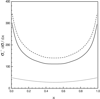
Figure 13: The dependence of $\sigma_{0}^{-1}d\sigma/dx$ on $x$ for a screened Coulomb potential, $\omega_{1}/m=1000$, $Z=83$. The dashed curve corresponds to the Born approximation, the solid one gives the exact result, and the dotted curve shows the difference between the Born cross section and the exact one.

In Fig. 14 the Coulomb corrections to the cross section $d\sigma_{c}/dx$ divided by $\sigma_{0}=0.782\cdot 10^{-9}Z^{2}$b are shown as a function of $Z$ for $x=0.7$ (solid line). Since their dependence on $x$ is rather weak ( see Fig. 13), this curve allows one to estimate the magnitude of the Coulomb corrections for any $x$. To elucidate the role of higher-order Coulomb corrections we plot also the first Coulomb correction to the cross section divided by $\sigma_{0}$ (dashed curve). This ratio is proportional to $Z^{2}$. As seen in Fig. 13, for sufficiently large $Z$ the first Coulomb correction is irrelevant to the complete result for these corrections.

Figure 14: The dependence of the Coulomb corrections $\sigma_{0}^{-1}d\sigma_{C}/dx$ on $Z$ for $x=0.7$; solid curve: complete result, dashed curve: first correction.

To conclude this Section, we emphasize that the proper description of photon splitting in the electric field of a heavy atom requires the exact account of this field. For large $Z$, the contribution of the Coulomb corrections is always noticeable, though the magnitude of the effect depends on the type of a cross section and kinematic conditions.

7. Experimental investigations of photon splitting

The observation of photon splitting is a difficult problem due to a smallness of its cross section as compared to those of other processes initiated by the initial photons in a target. The following background processes are significant: double Compton effect off the atomic electrons ($\gamma e\to\gamma\gamma e$), and the emission of two hard photons from $e^{+}e^{-}$ pair produced by the initial photon. The relative importance of these processes depends on the photon energy. For the energy $\omega_{1}\sim m$, where the search of photon splitting was undertaken in two experiments [16, 17], only double Compton scattering determines the background conditions. In these experiments, the photons from an intense radioactive source ($Zn^{65}$ with $\omega_{1}~{}\simeq~{}1.1$ MeV in [16], and $Co^{60}$ with $\omega_{1}~{}\simeq~{}1.17,\,1.33$ MeV in [17]) were used. The combination of the coincidence and energy-summing detection technique was applied. The number of events considered as candidates for photon splitting exceeded the theoretical expectations by the factor of 300 in [17], and by the factor of 6 in [16]. The role of the background process in [16] was unclear. Nevertheless, the authors of [16] concluded that their ”results for $Z\sim 28$ strongly indicate the existence of photon splitting”.

At high photon energy $\omega\gg m$ the emission of hard photons from $e^{+}e^{-}$ pair becomes most important as a background process. In 1973 the experiment devoted to the study of Delbrück scattering of photons in energy region $1\div 7$ GeV was performed [28]. The bremsstrahlung non-tagged photon beam was used. Some events were assigned by authors of [28] to the photon splitting process. As shown in [10, 29], the theoretical value for the number of photon splitting events under the conditions of the experiment was two orders of magnitude smaller than the experimental result. It was also argued that the events observed could be explained by the production of $e^{+}e^{-}$ pair and one hard photon.

The first successful observation of photon splitting was performed in 1995-96 using the tagged photon beam of the energy $120\div 450$ MeV at the VEPP-4M $e^{+}e^{-}$ collider [30] in the Budker Institute of Nuclear Physics (Novosibirsk). Another goal of this experiment was a study of Delbrück scattering [5]. The total statistics collected was $1.6\cdot 10^{9}$ incoming photons with BGO (bismuth germanate) target and $4\cdot 10^{8}$ photons without target for background measurements. The preliminary results were published in [18], [19]. Here we present the last data analysis for this experiment [20].

The experimental setup is shown in Fig. 15. Some ideas of this setup were suggested in [31]. The main features of the experimental approach are:

• The use of high-quality tagged photon beam produced by backward Compton scattering of laser light off high-energy electron beam. Thereby, the energy of the initial photon is accurately determined.

• Strong suppression of the background processes by means of the detection of charged particles produced in the target and in other elements of the photon-beam line.

• The detection of both final photons to discriminate the photon splitting events from those with one final photon produced in Compton or Delbrück scattering.

• The requirement of the balance between the sum of the energies of the final photons and the energy of the tagged initial photon. This provides the additional suppression of the events with charged particles missed by the detection system.

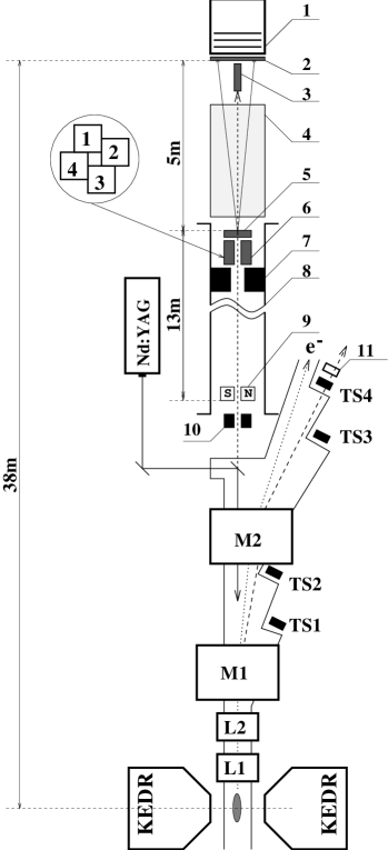
Figure 15: Principal scheme of setup: LKr calorimeter (1); scintillation veto-counter (2); beam dump (BGO) (3); He-filled tube (4m length) (4); target (BGO) (5); active collimator (BGO) (6); lead absorber (7); guiding tube for the gamma-quanta beam (8); cleaning magnet (9); passive lead collimator (10); TS scintillattion counter (11); Nd:YAG is the laser; TS1-TS4 are tagging system hodoscopes; M1 and M2 are bending magnets; L1 and L2 are quadrupole lenses.

At high energy of the initial photon $\omega_{1}\gg m$, the photon splitting cross section is peaked at small angles between momenta of all photons ($\sim m/\omega_{1}$). Therefore, a good collimation of the primary photon beam is required. The ROKK-1M facility [32] is used as the intense source of the tagged $\gamma$-quanta. The electron energy loss in the process of Compton scattering of laser light is measured by the tagging system (TS) [33] of the KEDR detector [34]. The TS consists of the focussing spectrometer formed by accelerator quadrupole lenses and bending magnets, and 4 hodoscopes of the drift tubes. High-energy photons move in a narrow cone around the electron beam direction. The angular spread is of the order $1/\gamma$, where $\gamma=E_{beam}/m$ is the relativistic factor of the electron beam. The photon energy spectrum has a sharp edge at

$$\omega_{th}=\frac{4\gamma^{2}\omega_{laser}}{1+4\gamma\omega_{laser}/m}\,,$$ (7..1)

that allows one to perform the absolute calibration of the tagging system in a wide energy range. In experiment the laser photon energy was $\omega_{laser}=1.165$ eV, the electron beam energy $E_{beam}=5.25$ GeV, and $\omega_{th}=450$ MeV. The photon energy resolution provided by the tagging system depends on the photon energy and on the position of scattered electron in TS hodoscope: it was 0.8 % at $\omega_{1}=450$ MeV (at the center of the hodoscope) and $\sim 5$ % at $\omega_{1}=120$ MeV (at the edge of the hodoscope). The collimation of the photon beam is provided by two collimators spaced at 13.5 m. The last collimator, intended to strip off the beam halo produced on the first one, is made of four BGO (bismuth germanate) crystals as shown in the separate view in Fig. 15. After passing through the collimation system, the photon beam hits $1X_{0}$ thick BGO crystal target.

Since one has to separate incident photons from those scattered in the target, certain angular region around the photon beam direction $\theta\leq\theta_{0}$ is enclosed by the dump made of 13 $X_{0}$ thick BGO crystal installed in front of the photon detector. The incoming photons which passed the target without interaction are absorbed by the dump, and the only photons to be detected are those scattered outside the dump shadow. For too large value of $\theta_{0}$, many photon splitting events would be lost while for too small value of $\theta_{0}$, the non-interacted photons would overwhelm the data acquisition system. As an optimum, the value $\theta_{0}=2.4$ mrad was chosen.

All active elements used in beam line (collimators, target, dump, scintillating veto counter) set a veto signal in the trigger and their signals are used in the analysis for background suppression. The information from the target and beam dump is also used for measurement of the incoming photon flux. The liquid-krypton ionization calorimeter is used for the detection of the final photons. Its three-layer double-sided electrode structure enables one to get both (X and Y) coordinates for detected photons. The energy resolution of the calorimeter is $2\,\%/\sqrt{\omega(\mbox{GeV})}$. The liquid-krypton calorimeter is described in details in [35, 36].

In the experiment, the detected final photons had the polar angles in the region $2.4~{}\mbox{mrad}\leq\theta\leq 20~{}\mbox{mrad}$. The corresponding cross section is called ”visible”. Fig. 16 shows the calculated energy dependence of the total ($a$) and visible ($b$) cross sections for various processes initiated by photons in BGO target: $e^{+}e^{-}$ pair production, Compton scattering on atomic electrons, Delbrück scattering, and photon splitting. The calculation of the photon splitting cross section was performed using the results obtained in [13, 14, 15].

Figure 16: The calculated energy dependence of the total (a) and the visible (b) cross sections of various processes initiated by photons in BGO target (in units of barn per one molecule of $Bi_{4}Ge_{3}O_{12}$).

In the event selection procedure the following constraints were applied:

• The absence of the signal caused by charge particles in all active elements of the photon-beam line.

• The balance of the tagged initial photon energy and the energy measured in the calorimeter within $3\sigma$ of its energy resolution.

• The existence of two separate tracks at least for one (X or Y) coordinate in the calorimeter strip structure. The track is found if there are close clusters in different layers.

The fulfillment of the latter requirement strongly suppresses the contribution of the processes with one photon in the final state which could imitate two photon events in the calorimeter.

The typical event which meets selection criteria is shown in Fig. 17. In this example two tracks are seen in both X and Y directions. The conversion of the first photon occurs in the Layer 1 while the second photon converts in the Layer 2.

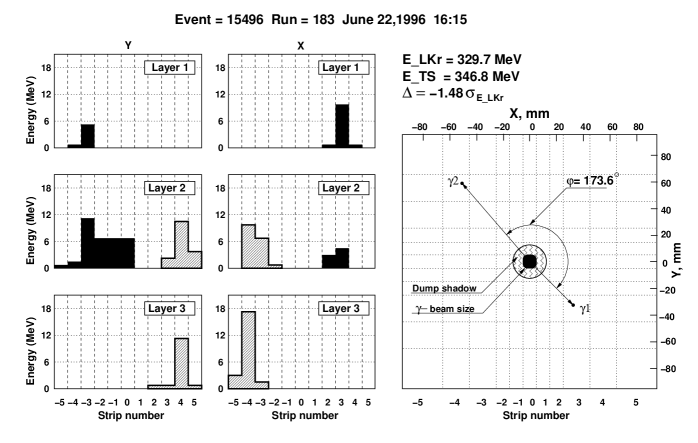
Figure 17: Energy profile in the calorimeter strip structure (left) and reconstructed kinematics (right) for a typical candidate to the photon splitting event.

The experimental results are presented in Tab. 1 and in Figs. 18, 19 together with the results of Monte-Carlo simulation based on the exact photon splitting cross section. The energy spectrum of the initial photons measured in the tagging system is shown in Fig.18(a). Tab. 1 and Fig. 19 present the data summed up over the initial photon spectrum. The errors shown in the Tab. 1 are statistical ones. The systematic error is determined by the accuracy of the measurement of the number of initial photons and by the uncertainty in the reconstruction efficiency of photon splitting events. The estimation of these systematic errors gives 2 % and 5 %, respectively.

Table 1: The number of reconstructed events. Here Q is the number of incoming photons. The quantity $N_{\phi<150^{\circ}}$ is the number of events with the complanarity angle ${\phi<150^{\circ}}$ (see Fig. 19), $N_{\phi>150^{\circ}}$ is the number of events with ${\phi>150^{\circ}}$. The quantities $N_{\phi<150^{\circ}}$ and $N_{\phi>150^{\circ}}$ are normalized to the experimental statistics collected with the target. MC means Monte-Carlo simulation.

DATA	TARGET	${\bf Q,\,{10^{9}}}$	$\bf N_{\phi>150^{\circ}}$	$\bf N_{\phi<150^{\circ}}$
Experiment	$\rm Bi_{4}Ge_{3}O_{12}$	1.63	336$\pm$18	82$\pm$9
Experiment	no target	0.37	10$\pm$3	10$\pm$3
MC photon splitting	$\rm Bi_{4}Ge_{3}O_{12}$	6.52	364$\pm$10	72$\pm$5
MC Delbrück scattering	$\rm Bi_{4}Ge_{3}O_{12}$	1.63	2$\pm$1	16$\pm$4
MC other backgrounds	$\rm Bi_{4}Ge_{3}O_{12}$	1.63	0	16$\pm$4

As seen from the Table 1 and Fig. 19a, the main part of the photon splitting events has, in agreement with the theory, a complanarity angle $\phi$ (the azimuth angle between final photon momenta) close to $180^{\circ}$. The choice of the interval $\phi>150^{\circ}$ allows us to improve the signal-to-background ratio (see, e.g., the last two rows of the Table 1). Just this $\phi$-interval was used to plot the distributions over polar angles in Fig. 19 and the dependence of the number of reconstructed photon splitting events on the initial photon energy $E_{TS}$ in Fig. 18(b). Note that for most of the events in this $\phi$-interval, the variable $\tilde{x}={\theta_{min}}/({\theta_{min}+\theta_{max}})$ is approximately equal to the ratio $\mbox{min}(\omega_{2},\,\omega_{3})/\omega_{1}$ since the main contribution to the cross section comes from the region $|\bm{k}_{2\perp}+\bm{k}_{3\perp}|\ll{k}_{2\perp},\,{k}_{3\perp}$, i.e. $\phi\approx 180^{\circ}$ and $\omega_{2}\theta_{2}\approx\omega_{3}\theta_{3}$.

Figure 18: (a) The photon energy spectrum measured in the tagging system (TS). (b) The number of reconstructed photon splitting events as a function of the tagged photon energy $E_{TS}$. In plot (b) black circles present the experimental results, histogram is the result of Monte-Carlo simulation based on the exact in $Z\alpha$ photon splitting cross section.

The results presented in the Table 1 and in Figs. 18(b), 19 show a good agreement between the theory and the experiment. More precisely, the total number of reconstructed events in the experiment (see Table 1) differs from the result of MC simulation by 1.5 standard deviations.

Figure 19: The number of the selected photon splitting events as a function of
the azimuth angle between momenta of the outgoing photons (a);
the polar angle $\theta_{min}=\mbox{min}\{\theta_{2},\theta_{3}\}$ (b);
the polar angle $\theta_{max}=\mbox{max}\{\theta_{2},\theta_{3}\}$ (c);
the variable $\tilde{x}={\theta_{min}}/({\theta_{min}+\theta_{max}})$ (d).
In figures (b), (c), and (d) only events satisfying the complanarity cut $\phi\geq 150^{\circ}$ (see plot (a)) are included. Black circles present the experimental results, histograms are the results of Monte-Carlo simulation based on the exact in $Z\alpha$ photon splitting cross section.

Figure 20: The visible photon splitting cross section calculated exactly in $Z\alpha$ (1) and in the Born approximation(2) as a function of the initial photon energy.

In order to demonstrate the role of the Coulomb corrections under the experimental conditions, we show in Fig. 20 the visible cross sections calculated exactly in $Z\alpha$ and in the Born approximation as a function of the initial photon energy. For all energies considered, the Born result exceeds the exact one by 20 % approximately. Therefore, the use of the Born cross section for MC simulation would lead to the disagreement between the theory and the experiment of 3.5 standard deviations. In other words, the experimental results are significantly closer to predictions of the exact theory than to those obtained in the Born approximation.

We conclude that the high-energy photon splitting in the atomic fields is reliably observed and well investigated. This nonlinear QED process is also studied in detail theoretically. At present, the experiment and the theory are consistent within the achieved experimental accuracy.

Appendix Appendix  A

In this Appendix we present the result of [1] for the amplitudes of photon-photon scattering entering (4..4)

$$M_{++++} = {8\alpha^{2}}\Biggl{\{}-1-\left(2+\frac{4\beta}{\zeta}\right)Q(\beta)-\left(2+\frac{4\gamma}{\zeta}\right)Q(\gamma)$$

$$-\left[\frac{2(\beta^{2}+\gamma^{2})}{\zeta^{2}}+\frac{8}{\zeta}\right][T(\beta)+T(\gamma)]-\frac{4}{\beta}\left(1+\frac{2}{\zeta}\right)I(\zeta,\beta)$$

$$-\frac{4}{\gamma}\left(1+\frac{2}{\zeta}\right)I(\zeta,\gamma)+\left[\frac{2(\beta^{2}+\gamma^{2})}{\zeta^{2}}+\frac{16}{\zeta}+\frac{4}{\beta}+\frac{4}{\gamma}-\frac{8}{tu}\right]I(\beta,\gamma)\Biggr{\}}\,,$$

$$M_{+++-} = {8\alpha^{2}}\Biggl{\{}1-4\left(\frac{1}{\zeta}+\frac{1}{\beta}+\frac{1}{\gamma}\right)[T(\zeta)+T(\beta)+T(\gamma)]$$

$$+4\left(\frac{1}{\gamma}-\frac{2}{st}\right)I(\zeta,\beta)+4\left(\frac{1}{\beta}-\frac{2}{su}\right)I(\zeta,\gamma)+4\left(\frac{1}{\zeta}-\frac{2}{tu}\right)I(\beta,\gamma)\Biggr{\}}\,,$$

$$M_{++--} = {8\alpha^{2}}\Biggl{\{}1-\frac{8}{st}I(\zeta,\beta)-\frac{8}{su}I(\zeta,\gamma)-\frac{8}{tu}I(\beta,\gamma)\Biggr{\}}\,,$$

$$M_{+-+-} = M_{++++}(\zeta\leftrightarrow\gamma)\,,\quad M_{+--+}=M_{++++}(\zeta\leftrightarrow\beta)\,.$$ (A.1)

Here

$$Q(x)=\sqrt{1+\frac{4}{x-i0}}\,\textrm{arcsinh}\left(\frac{\sqrt{x-i0}}{2}\right)-1\,,\quad T(x)=\textrm{arcsinh}^{2}\left(\frac{\sqrt{x-i0}}{2}\right)\,,$$

$$I(x,y)=\frac{1}{4}\int\limits_{0}^{1}d\tau\frac{\ln[1+x\tau(1-\tau)-i0]+\ln[1+y\tau(1-\tau)-i0]}{\tau(1-\tau)+(x+y)/xy}$$

$$\zeta=-\frac{2k_{2}k_{3}}{m^{2}}=-\frac{k_{2\perp}^{2}}{m^{2}x(1-x)}\,,\ \beta=\frac{2k_{1}k_{2}}{m^{2}}=\frac{k_{2\perp}^{2}}{m^{2}x}\,,\ \gamma=\frac{2k_{1}k_{3}}{m^{2}}=\frac{k_{2\perp}^{2}}{m^{2}(1-x)}\,.$$ (A.2)

In the expressions for $\zeta$, $\beta$, and $\gamma$ we took into account the smallness of $\theta_{2,3}$ and the relation $\bm{k}_{3\perp}=-\bm{k}_{2\perp}$, which is valid in the region of applicability of the WW approximation.

The asymptotics of (Appendix  A) at $|\zeta|,\beta,\gamma\ll 1$ reads

$$M_{++++} \approx \frac{11\alpha^{2}}{45}\zeta^{2}\,,\quad M_{+--+}\approx\frac{11\alpha^{2}}{45}\beta^{2}\,,\quad M_{+-+-}\approx\frac{11\alpha^{2}}{45}\gamma^{2}\,,$$

$$M_{++--} \approx -\frac{\alpha^{2}}{15}(\zeta^{2}+\beta^{2}+\gamma^{2})\,,\quad M_{+++-}\approx 0\,.$$ (A.3)

At $|\zeta|,\beta,\gamma\gg 1$ one has

$$M_{++++} = 8\alpha^{2}\left\{-1+(1-2x)\ln[1/x-1]-(x^{2}-x+1/2)(\ln^{2}[1/x-1]+\pi^{2})\right\}\,,$$

$$M_{+--+} = M_{++++}(x\to 1/(1-x+i0))\,,\quad M_{+-+-}=M_{++++}(x\to 1/(x+i0))\,,$$

$$M_{++--} = M_{+++-}=8\alpha^{2}\,.$$ (A.4)

Appendix Appendix  B

In this Appendix we present the functions $x_{i}$ and $y_{i}$ which appear in the result for the Born cross section (5..1) obtained in [6] and later rederived in [2].

$$x_{1} = \zeta\left[\left({2\zeta\over\beta}+{2\gamma-\zeta\over\beta+\gamma}-{2\zeta\beta\over(\beta+\gamma)^{2}}\right){\omega_{1}\over m}+\gamma\left({2\over\beta}+{1\over\beta+\gamma}\right){\omega_{2}\over m}\right.$$

$$\left.-{\beta\over\beta+\gamma}{\omega_{3}\over m}\right][A(\zeta)-A(\delta)]-\left[\gamma\left({\zeta\gamma\over\beta^{2}}+{\zeta-\gamma-2\over 2\beta}-{1\over\beta+\gamma}\right){\omega_{2}\over m}\right.$$

$$\left.+\zeta\left({\zeta\gamma\over\beta^{2}}-{\zeta-\gamma\over 2\beta}-{1\over\zeta}-{1\over\beta}-{1\over\gamma}+{1\over\beta+\gamma}+{2\beta\over(\beta+\gamma)^{2}}\right){\omega_{1}\over m}\right.$$

$$\left.-\beta\left({\zeta-\gamma\over 2\beta}+{\beta\over\gamma(\beta+\gamma)}\right){\omega_{3}\over m}\right]B(\zeta)+\left[{\zeta(\beta-\gamma)\over\beta\gamma}{\omega_{1}\over m}+{\beta\over\gamma}{\omega_{3}\over m}\right]B(\beta)$$

$$+\zeta\left[\left({\zeta\gamma\over\beta^{2}}-{\zeta-\gamma\over 2\beta}-{1\over\beta}-{1\over\gamma}-{1\over\zeta+\beta}+{1\over\beta+\gamma}+{2\beta\over(\beta+\gamma)^{2}}\right){\omega_{1}\over m}\right.$$

$$\left.-\beta\left({1\over 2\beta}+{\beta\delta\over\zeta\gamma(\zeta+\beta)(\beta+\gamma)}\right){\omega_{3}\over m}\right]B(\delta)+{2\zeta\gamma\over\beta+\gamma}{\omega_{1}\over m}$$

$$-2\left[{\zeta(\zeta+\gamma)\over\beta\gamma}{\omega_{1}\over m}+{(\zeta-\beta)(\zeta+\gamma)\over\zeta\beta}{\omega_{2}\over m}+\left({\beta\over\zeta}+{\zeta\over\gamma}\right){\omega_{3}\over m}\right]S(\zeta,\beta,\gamma)$$

$$-\zeta\left[\left({2\zeta\gamma\over\beta^{2}}+{\gamma-\zeta-6\over\beta}-{4\over\zeta}+{2\over\gamma}\right){\omega_{1}\over m}-\left(1-{2\beta\over\zeta\gamma}\right){\omega_{3}\over m}\right]S(\beta,\zeta,\gamma)$$

$$+(\zeta\leftrightarrow\gamma,\omega_{1}\leftrightarrow\omega_{2},\omega_{3}\rightarrow-\omega_{3})\,,$$

$$x_{4} = \left[{\zeta\over\gamma}{\omega_{1}\over m}-{\gamma(\zeta-\beta)\over\zeta\beta}{\omega_{2}\over m}\right][B(\zeta)+B(\beta)+B(\gamma)-B(\delta)]+{2(\zeta+\gamma)\over\zeta}{\omega_{2}\over m}S(\zeta,\beta,\gamma)$$

$$-{2\over\beta}\left[(\zeta+\beta){\omega_{1}\over m}+(\beta+\gamma){\omega_{2}\over m}\right]S(\beta,\zeta,\gamma)-(\beta\leftrightarrow\gamma,\,\omega_{2}\leftrightarrow\omega_{3})\,,$$

$$x_{2} = x_{1}(\beta\leftrightarrow\gamma,\,\omega_{2}\leftrightarrow\omega_{3})\,,\quad x_{3}=x_{1}(\zeta\leftrightarrow\beta,\,\omega_{3}\leftrightarrow-\omega_{1})\,.$$ (B.1)

$$y_{1} = -2\left({1\over\zeta}+{\zeta+\gamma-4\over\beta\gamma}\right)S(\zeta,\beta,\gamma)+\left({\zeta\gamma\over\beta^{2}}+{\zeta-5\over\beta}+{4-2\zeta\over\zeta\gamma}\right)S(\beta,\zeta,\gamma)$$

$$-\zeta\left({2\over\beta}-{1\over\beta+\gamma}\right)[A(\zeta)-A(\delta)]+\left({\zeta\gamma\over\beta^{2}}+{\zeta+\gamma-6\over 2\beta}-{\beta\over\gamma(\beta+\gamma)}\right)B(\zeta)$$

$$-\left({\zeta\gamma\over 2\beta^{2}}+{\zeta+\gamma-6\over 4\beta}-{\beta\over\gamma(\beta+\gamma)}\right)B(\delta)-\left({1\over\zeta}+{1\over 2\beta}\right)B(\beta)+(\zeta\leftrightarrow\gamma)\,,$$

$$y_{4} = 2-({1\over\zeta}+{1\over\beta}+{1\over\gamma})[B(\zeta)+B(\beta)+B(\gamma)-B(\delta)]$$

$$-{2\over\zeta}\left(1-{4\zeta\over\beta\gamma}\right)S(\zeta,\beta,\gamma)-{2\over\beta}\left(1-{4\beta\over\zeta\gamma}\right)S(\beta,\zeta,\gamma)-{2\over\gamma}\left(1-{4\gamma\over\zeta\beta}\right)S(\gamma,\zeta,\beta)\,,$$

$$y_{2} = y_{1}(\zeta\leftrightarrow\beta)\,,\quad y_{3}=y_{1}(\gamma\leftrightarrow\beta)\,.$$ (B.2)

Here $\delta=\zeta+\beta+\gamma$ and the functions $A$, $B$, and $S$ are defined as

$$A(u)=\int\limits_{0}^{1}dx\,\ln[1-i0+u\,x(1-x)]\,,\quad B(u)=\int\limits_{0}^{1}{dx\over x(1-x)}\ln[1-i0+u\,x(1-x)]\,,$$

$$S(u,v,w)=\frac{1}{2}\int\limits_{0}^{1}\frac{dx\,v\,w}{u-v\,w\,x(1-x)}\ln\left\{\frac{[1-i0+v\,x(1-x)][1-i0+w\,x(1-x)]}{1+(u+v+w)x(1-x)}\right\}\,.$$

In fact, the functions $A(u)$ and $B(u)$ are expressed via elementary functions and $S(u,v,w)$ is expressed in terms of dilogarithmic functions [6].

Appendix Appendix  C

In this Appendix we present some results obtained in [11] for the total ($\sigma$) and differential ($d\sigma/dx$) cross sections of photon splitting in a screened and Coulomb potentials. The form factor used in the calculations was taken from [27].

Table C.2: The total Born cross section $\sigma$ in units of $Z^{2}\mathrm{(nb)}$ for a Coulomb potential (row $Z=0$) and screened potential as a function of $\omega_{1}$ and $Z$. The dependence on $Z$ is due to the atomic form factor.

$\quad\omega_{1}/m$	$1$	$3$	$10$	$30$	$100$	$300$	$1000$	$3000$
$Z$
$0$	$1.436\times 10^{-3}$	$0.795$	$12.10$	$31.47$	$56.5$	$80.6$	$107.3$	$131.8$
$1$	$1.436\times 10^{-3}$	$0.795$	$12.10$	$31.47$	$56.4$	$79.0$	$97.9$	$107.6$
$10$	$1.431\times 10^{-3}$	$0.795$	$12.08$	$31.13$	$54.1$	$72.0$	$84.5$	$90.9$
$20$	$1.423\times 10^{-3}$	$0.794$	$12.03$	$30.83$	$52.98$	$69.58$	$81.18$	$87.2$
$50$	$1.40\times 10^{-3}$	$0.790$	$11.92$	$30.32$	$51.32$	$66.32$	$75.72$	$81.0$
$68$	$1.39\times 10^{-3}$	$0.787$	$11.85$	$30.04$	$50.54$	$64.92$	$74.22$	$78.09$
$92$	$1.378\times 10^{-3}$	$0.782$	$11.78$	$29.71$	$49.74$	$63.33$	$72.07$	$75.50$

Table C.3: The Born cross section $d\sigma/dx$ in units of $Z^{2}\mathrm{(b)}$ as a function of $x=\omega_{2}/\omega_{1}$ for different $\omega_{1}$. The column $Z=0$ corresponds to the a Coulomb potential.

$Z$	$0$	$20$	$50$	$82$	$92$
$x$
$\omega_{1}=m$
$0.00993$	$1.78\times 10^{-15}$	$1.59\times 10^{-15}$	$1.50\times 10^{-15}$	$1.44\times 10^{-15}$	$1.42\times 10^{-15}$
$0.0508$	$1.36\times 10^{-13}$	$1.27\times 10^{-13}$	$1.22\times 10^{-13}$	$1.19\times 10^{-13}$	$1.17\times 10^{-13}$
$0.119$	$9.09\times 10^{-13}$	$8.84\times 10^{-13}$	$8.63\times 10^{-13}$	$8.47\times 10^{-13}$	$8.41\times 10^{-13}$
$0.204$	$2.42\times 10^{-12}$	$2.39\times 10^{-12}$	$2.34\times 10^{-12}$	$2.31\times 10^{-12}$	$2.30\times 10^{-12}$
$0.296$	$3.88\times 10^{-12}$	$3.85\times 10^{-12}$	$3.79\times 10^{-12}$	$3.74\times 10^{-12}$	$3.73\times 10^{-12}$
$0.381$	$4.78\times 10^{-12}$	$4.74\times 10^{-12}$	$4.68\times 10^{-12}$	$4.63\times 10^{-12}$	$4.61\times 10^{-12}$
$0.449$	$5.09\times 10^{-12}$	$5.06\times 10^{-12}$	$4.99\times 10^{-12}$	$4.93\times 10^{-12}$	$4.92\times 10^{-12}$
$0.49$	$5.08\times 10^{-12}$	$5.05\times 10^{-12}$	$4.98\times 10^{-12}$	$4.93\times 10^{-12}$	$4.91\times 10^{-12}$
$\omega_{1}=10m$
$0.00993$	$1.84\times 10^{-9}$	$1.79\times 10^{-9}$	$1.76\times 10^{-9}$	$1.73\times 10^{-9}$	$1.72\times 10^{-9}$
$0.0508$	$2.51\times 10^{-8}$	$2.49\times 10^{-8}$	$2.46\times 10^{-8}$	$2.44\times 10^{-8}$	$2.43\times 10^{-8}$
$0.119$	$2.76\times 10^{-8}$	$2.75\times 10^{-8}$	$2.72\times 10^{-8}$	$2.70\times 10^{-8}$	$2.69\times 10^{-8}$
$0.204$	$2.64\times 10^{-8}$	$2.63\times 10^{-8}$	$2.60\times 10^{-8}$	$2.58\times 10^{-8}$	$2.57\times 10^{-8}$
$0.296$	$2.51\times 10^{-8}$	$2.49\times 10^{-8}$	$2.47\times 10^{-8}$	$2.45\times 10^{-8}$	$2.44\times 10^{-8}$
$0.381$	$2.42\times 10^{-8}$	$2.41\times 10^{-8}$	$2.39\times 10^{-8}$	$2.37\times 10^{-8}$	$2.36\times 10^{-8}$
$0.449$	$2.39\times 10^{-8}$	$2.37\times 10^{-8}$	$2.35\times 10^{-8}$	$2.33\times 10^{-8}$	$2.32\times 10^{-8}$
$0.49$	$2.38\times 10^{-8}$	$2.37\times 10^{-8}$	$2.34\times 10^{-8}$	$2.32\times 10^{-8}$	$2.32\times 10^{-8}$
$\omega_{1}=100m$
$0.00993$	$1.65\times 10^{-7}$	$1.56\times 10^{-7}$	$1.52\times 10^{-7}$	$1.48\times 10^{-7}$	$1.47\times 10^{-7}$
$0.0508$	$1.49\times 10^{-7}$	$1.40\times 10^{-7}$	$1.36\times 10^{-7}$	$1.33\times 10^{-7}$	$1.32\times 10^{-7}$
$0.119$	$1.28\times 10^{-7}$	$1.20\times 10^{-7}$	$1.16\times 10^{-7}$	$1.13\times 10^{-7}$	$1.13\times 10^{-7}$
$0.204$	$1.11\times 10^{-7}$	$1.04\times 10^{-7}$	$1.01\times 10^{-7}$	$9.83\times 10^{-8}$	$9.76\times 10^{-8}$
$0.296$	$1.01\times 10^{-7}$	$9.39\times 10^{-8}$	$9.09\times 10^{-8}$	$8.86\times 10^{-8}$	$8.80\times 10^{-8}$
$0.381$	$9.48\times 10^{-8}$	$8.85\times 10^{-8}$	$8.56\times 10^{-8}$	$8.35\times 10^{-8}$	$8.29\times 10^{-8}$
$0.449$	$9.26\times 10^{-8}$	$8.64\times 10^{-8}$	$8.36\times 10^{-8}$	$8.15\times 10^{-8}$	$8.09\times 10^{-8}$
$0.49$	$9.21\times 10^{-8}$	$8.59\times 10^{-8}$	$8.31\times 10^{-8}$	$8.10\times 10^{-8}$	$8.05\times 10^{-8}$
$\omega_{1}=1000m$
$0.00993$	$3.73\times 10^{-7}$	$2.96\times 10^{-7}$	$2.77\times 10^{-7}$	$2.69\times 10^{-7}$	$2.65\times 10^{-7}$
$0.0508$	$3.01\times 10^{-7}$	$2.33\times 10^{-7}$	$2.18\times 10^{-7}$	$2.11\times 10^{-7}$	$2.08\times 10^{-7}$
$0.119$	$2.44\times 10^{-7}$	$1.85\times 10^{-7}$	$1.73\times 10^{-7}$	$1.67\times 10^{-7}$	$1.65\times 10^{-7}$
$0.204$	$2.06\times 10^{-7}$	$1.54\times 10^{-7}$	$1.44\times 10^{-7}$	$1.39\times 10^{-7}$	$1.37\times 10^{-7}$
$0.296$	$1.83\times 10^{-7}$	$1.36\times 10^{-7}$	$1.27\times 10^{-7}$	$1.22\times 10^{-7}$	$1.21\times 10^{-7}$
$0.381$	$1.71\times 10^{-7}$	$1.27\times 10^{-7}$	$1.18\times 10^{-7}$	$1.14\times 10^{-7}$	$1.12\times 10^{-7}$
$0.449$	$1.67\times 10^{-7}$	$1.23\times 10^{-7}$	$1.15\times 10^{-7}$	$1.11\times 10^{-7}$	$1.09\times 10^{-7}$
$0.49$	$1.66\times 10^{-7}$	$1.23\times 10^{-7}$	$1.14\times 10^{-7}$	$1.10\times 10^{-7}$	$1.08\times 10^{-7}$

Appendix Appendix  D

Here we present the photon splitting amplitudes exact in the parameter $Z\alpha$ and valid in the high-energy zero-mass limit ($\omega_{2}\theta_{2},\,\omega_{3}\theta_{3}\gg m$ and $\theta_{2,3}\ll 1$) [14]. They read

$$M=\frac{4e^{3}Z\alpha}{\pi\omega_{1}\omega_{2}\omega_{3}{\Delta}^{2}}\int\limits_{-1}^{1}\frac{dy\,\,\mbox{sign}\,y}{1-y^{2}}\,\left[\mbox{Re}\left(\frac{1+y}{1-y}\right)^{iZ\alpha}\right]\,R\,;$$

$$R_{+--}=\frac{q^{2}}{(\bm{e}^{*}\cdot\bm{\theta}_{3})(\bm{e}^{*}\cdot\bm{\theta}_{23})}\int\limits_{0}^{\omega_{2}}\!d\varepsilon\,\kappa_{2}\,\bm{e}^{*}\cdot(\kappa_{2}\bm{\theta}_{2}-\bm{\Delta})\,\frac{\vartheta(\bm{r}^{2}-q^{2})}{(\bm{e}^{*}\cdot\bm{r})^{2}}\,+\,{{\omega_{2}\leftrightarrow\omega_{3}}\choose{\bm{\theta}_{2}\leftrightarrow\bm{\theta}_{3}}}\,,$$

$$R_{+++}=\int\limits_{0}^{\omega_{2}}\!d\varepsilon\,\Biggl{[}\frac{\omega_{3}\varepsilon\kappa_{2}}{\omega_{2}}\left(\frac{s}{t}-1\right)\left(\frac{\omega_{3}}{(\bm{e}\cdot\bm{u})}-\frac{8(\bm{e}^{*}\cdot\bm{\theta}_{3})(\kappa_{2}^{2}+\kappa_{3}^{2})}{s-t-4(\bm{e}^{*}\cdot\bm{r})(\bm{e}\cdot\bm{u})}\right)$$

$$+\vartheta(q^{2}-{r}^{2})\frac{(\kappa_{2}^{2}+\kappa_{3}^{2})\kappa_{2}(1+1/y)(\bm{e}^{*}\cdot\bm{\theta}_{2})(\bm{e}\cdot\bm{\Delta})}{(\bm{e}\cdot\bm{\theta}_{23})[\varepsilon(\bm{e}^{*}\cdot\bm{r})(\bm{e}\cdot\bm{\theta}_{23})-\kappa_{2}(1+1/y)(\bm{e}\cdot\bm{\Delta})(\bm{e}^{*}\cdot\bm{\theta}_{2})]}\Biggr{]}\,+\,{{\omega_{2}\leftrightarrow\omega_{3}}\choose{\bm{\theta}_{2}\leftrightarrow\bm{\theta}_{3}}}\,,$$

$$R_{++-}=\int\limits_{0}^{\omega_{2}}\!d\varepsilon\,\Biggl{[}\frac{\omega_{3}\kappa_{2}\kappa_{3}}{\omega_{1}}\left(\frac{is_{1}}{t_{1}}-1\right)\left(\frac{\kappa_{2}-\varepsilon}{(\bm{e}^{*}\cdot\bm{u}_{1})}+\frac{8(\bm{e}\cdot\bm{\theta}_{23})(\kappa_{2}^{2}+\varepsilon^{2})}{s_{1}+it_{1}-4(\bm{e}\cdot\bm{r})(\bm{e}^{*}\cdot\bm{u}_{1})}\right)$$

$$+\vartheta(q^{2}-{r}^{2})\frac{(\kappa_{2}^{2}+\varepsilon^{2})\kappa_{2}(1+1/y)(\bm{e}\cdot\bm{\theta}_{2})(\bm{e}^{*}\cdot\bm{\Delta})}{(\bm{e}^{*}\cdot\bm{\theta}_{3})[\kappa_{3}(\bm{e}\cdot\bm{r})(\bm{e}^{*}\cdot\bm{\theta}_{3})-\kappa_{2}(1+1/y)(\bm{e}^{*}\cdot\bm{\Delta})(\bm{e}\cdot\bm{\theta}_{2})]}\Biggr{]}$$

$$-\omega_{2}\int\limits_{-\omega_{3}}^{0}\!d\varepsilon\,\kappa_{3}\Biggl{[}\frac{(\bm{e}\cdot\bm{\Delta})}{\omega_{1}(\bm{e}^{*}\cdot\bm{\Delta})}\left(\frac{is_{1}}{t_{1}}-1\right)\left(\frac{\varepsilon\kappa_{3}+\kappa_{2}^{2}}{(\bm{e}\cdot\bm{u}_{1})}+\frac{8(\bm{e}^{*}\cdot\bm{\theta}_{23})\kappa_{3}(\kappa_{2}^{2}+\varepsilon^{2})}{s_{1}-it_{1}-4(\bm{e}^{*}\cdot\bm{r}_{1})(\bm{e}\cdot\bm{u}_{1})}\right)$$

$$+\frac{(\bm{e}\cdot\bm{\Delta})}{\omega_{3}(\bm{e}^{*}\cdot\bm{\Delta})}\left(\frac{s_{2}}{t_{2}}-1\right)\left(\frac{\kappa_{2}\kappa_{3}-\varepsilon^{2}}{(\bm{e}\cdot\bm{u}_{2})}+\frac{8(\bm{e}^{*}\cdot\bm{\theta}_{2})\kappa_{3}(\kappa_{2}^{2}+\varepsilon^{2})}{s_{2}+t_{2}-4(\bm{e}^{*}\cdot\bm{r}_{1})(\bm{e}\cdot\bm{u}_{2})}\right)$$

$$+\vartheta({r}^{2}_{1}-q^{2})\frac{q^{2}(\kappa_{2}^{2}+\varepsilon^{2})}{2\omega_{2}(\bm{e}^{*}\cdot\bm{r}_{1})}\Biggl{(}\frac{1}{\kappa_{2}(\bm{e}^{*}\cdot\bm{r}_{1})(\bm{e}\cdot\bm{\theta}_{2})-\kappa_{3}(1/y-1)(\bm{e}\cdot\bm{\Delta})(\bm{e}^{*}\cdot\bm{\theta}_{3})}$$

$$+\frac{1}{\varepsilon(\bm{e}^{*}\cdot\bm{r}_{1})(\bm{e}\cdot\bm{\theta}_{23})-\kappa_{3}(1/y-1)(\bm{e}\cdot\bm{\Delta})(\bm{e}^{*}\cdot\bm{\theta}_{3})}\Biggr{)}\Biggr{]}\,,$$ (D.1)

$$\bm{u}=\bm{\Delta_{\perp}}\left(\frac{1}{y}-1+\frac{2\kappa_{2}}{\omega_{2}}\right)\,,\quad\bm{u}_{1}=\bm{\Delta_{\perp}}\left(\frac{1}{y}-1+\frac{2\kappa_{2}}{\omega_{1}}\right)\,,\quad\bm{u}_{2}=\bm{\Delta_{\perp}}\left(\frac{1}{y}-1-\frac{2\varepsilon}{\omega_{3}}\right)\,,\,$$

$$q^{2}={\Delta_{\perp}}^{2}(1/y^{2}-1)\,,\quad\bm{r}=\bm{\Delta_{\perp}}(1/y-1)+2\kappa_{2}\bm{\theta}_{2}\,,\quad\bm{r}_{1}=\bm{\Delta_{\perp}}(1/y+1)-2\kappa_{3}\bm{\theta}_{3}\,,$$

$$\bm{\theta}_{23}=\bm{\theta}_{2}-\bm{\theta}_{3}\,,\quad\kappa_{2}=\omega_{2}-\varepsilon\,,\quad\kappa_{3}=\omega_{3}+\varepsilon\,,\quad s={u}^{2}+q^{2}+\frac{4\omega_{1}\omega_{3}\kappa_{2}\varepsilon}{\omega_{2}^{2}}{\theta}_{3}^{2}\,,$$

$$s_{1}={u}_{1}^{2}+q^{2}-\frac{4\omega_{2}\omega_{3}\kappa_{2}\kappa_{3}}{\omega_{1}^{2}}{\theta}_{23}^{2}\,-i0\,,\quad s_{2}={u}_{2}^{2}+q^{2}-\frac{4\omega_{1}\omega_{2}\kappa_{3}\varepsilon}{\omega_{3}^{2}}{\theta}_{2}^{2}\,$$

$$t=\sqrt{s^{2}-4q^{2}{u}^{2}}\,,\quad t_{1}=\sqrt{4q^{2}{u}_{1}^{2}-s_{1}^{2}}\,,\quad t_{2}=\sqrt{s_{2}^{2}-4q^{2}{u}_{2}^{2}}\,.$$ (D.2)

In the Born approximation (linear in $Z\alpha$ term of (Appendix  D)) all integrals can be taken with the result

$$M_{+--}=\frac{2Z\alpha e^{3}[(\bm{e}^{*}\cdot\bm{\theta}_{2})(\bm{e}\cdot\bm{\theta}_{3})-(\bm{e}\cdot\bm{\theta}_{2})(\bm{e}^{*}\cdot\bm{\theta}_{3})]}{\pi{\Delta}^{2}(\bm{e}^{*}\cdot\bm{\theta}_{2})(\bm{e}^{*}\cdot\bm{\theta}_{3})(\bm{e}^{*}\cdot\bm{\theta}_{23})}\,,$$

$$M_{+++}=\frac{2(Z\alpha)e^{3}\omega_{1}}{\pi{\Delta}^{2}(\bm{e}\cdot\bm{\theta}_{23})^{2}\omega_{2}\omega_{3}}\Biggl{\{}(\bm{e}\cdot\bm{\Delta})\Biggl{[}1+\frac{(\bm{e}\cdot\bm{\theta}_{2})+(\bm{e}\cdot\bm{\theta}_{3})}{(\bm{e}\cdot\bm{\theta}_{23})}\ln({a_{2}\over a_{3}})$$

$$+\frac{(\bm{e}\cdot\bm{\theta}_{2})^{2}+(\bm{e}\cdot\bm{\theta}_{3})^{2}}{(\bm{e}\cdot\bm{\theta}_{23})^{2}}\left({\pi^{2}\over 6}+{1\over 2}\ln^{2}({a_{2}\over a_{3}})+\mbox{Li}_{2}(1-a_{2})+\mbox{Li}_{2}(1-a_{3})\right)\Biggr{]}$$

$$+{1\over(\bm{e}\cdot\bm{\Delta})}\left[\omega_{3}^{2}(\bm{e}\cdot\bm{\theta}_{3})^{2}\frac{a_{2}}{1-a_{2}}\left(1+{a_{2}\,\ln(a_{2})\over 1-a_{2}}\right)+\omega_{2}^{2}(\bm{e}\cdot\bm{\theta}_{2})^{2}\frac{a_{3}}{1-a_{3}}\right.$$

$$\left.\times\left(1+{a_{3}\,\ln(a_{3})\over 1-a_{3}}\right)\right]+\frac{2(\bm{e}\cdot\bm{\theta}_{2})(\bm{e}\cdot\bm{\theta}_{3})}{(\bm{e}\cdot\bm{\theta}_{23})}\left[\omega_{3}{a_{2}\,\ln(a_{2})\over 1-a_{2}}-\omega_{2}{a_{3}\,\ln(a_{3})\over 1-a_{3}}\right]\Biggr{\}}\,,$$

$$M_{++-}=\frac{2(Z\alpha)e^{3}\omega_{2}}{\pi{\Delta}^{2}(\bm{e}^{*}\cdot\bm{\theta}_{3})^{2}\omega_{1}\omega_{3}}\Biggl{\{}(\bm{e}^{*}\cdot\bm{\Delta})\Biggl{[}1-\frac{(\bm{e}^{*}\cdot\bm{\theta}_{2})+(\bm{e}^{*}\cdot\bm{\theta}_{23})}{(\bm{e}^{*}\cdot\bm{\theta}_{3})}\ln({-a_{1}\over a_{2}})$$

$$+\frac{(\bm{e}^{*}\cdot\bm{\theta}_{2})^{2}+(\bm{e}^{*}\cdot\bm{\theta}_{23})^{2}}{(\bm{e}^{*}\cdot\bm{\theta}_{3})^{2}}\left({\pi^{2}\over 6}+{1\over 2}\ln^{2}({-a_{1}\over a_{2}})+\mbox{Li}_{2}(1-a_{2})+\mbox{Li}_{2}(1+a_{1})\right)\Biggr{]}$$

$$+{1\over(\bm{e}^{*}\cdot\bm{\Delta})}\left[\omega_{3}^{2}(\bm{e}^{*}\cdot\bm{\theta}_{23})^{2}\frac{a_{2}}{1-a_{2}}\left(1+{a_{2}\,\ln(a_{2})\over 1-a_{2}}\right)-\omega_{1}^{2}(\bm{e}^{*}\cdot\bm{\theta}_{2})^{2}\frac{a_{1}}{1+a_{1}}\right.$$

$$\left.\times\left(1-{a_{1}\,\ln(-a_{1})\over 1+a_{1}}\right)\right]+\frac{2(\bm{e}^{*}\cdot\bm{\theta}_{2})(\bm{e}^{*}\cdot\bm{\theta}_{23})}{(\bm{e}^{*}\cdot\bm{\theta}_{3})}\left[\omega_{1}{a_{1}\,\ln(-a_{1})\over 1+a_{1}}-\omega_{3}{a_{2}\,\ln(a_{2})\over 1-a_{2}}\right]\Biggr{\}}\,,$$ (D.3)

where

$$a_{1}=\frac{{\Delta_{\perp}}^{2}}{\omega_{2}\omega_{3}\theta_{23}^{2}}-i0\,,\quad a_{2}=\frac{{\Delta_{\perp}}^{2}}{\omega_{1}\omega_{2}\theta_{2}^{2}}\,,\quad a_{3}=\frac{{\Delta_{\perp}}^{2}}{\omega_{1}\omega_{3}\theta_{3}^{2}}\,,\quad\mathrm{Li}_{2}(x)=-\int\limits_{0}^{x}\frac{dt}{t}\ln(1-t)\,.$$

Let us introduce the variable $\bm{\varrho}=(\omega_{2}\bm{\theta}_{2}-\omega_{3}\bm{\theta}_{3})/2$. If $\Delta\ll\varrho$ then the asymptotics of (Appendix  D) has the form

$$M_{+--} = \frac{4N(\bm{e}\cdot\bm{\varrho})^{3}}{{\varrho}^{4}}[(\bm{e}^{*}\cdot\bm{\Delta})(\bm{e}\cdot\bm{\varrho})-(\bm{e}\cdot\bm{\Delta})(\bm{e}^{*}\cdot\bm{\varrho})]\quad,\quad N=\frac{4Z\alpha{e^{3}}\omega_{2}\omega_{3}}{\pi\omega_{1}{\Delta}^{2}{\varrho}^{2}}\,;$$

$$M_{+++} = N\Biggl{[}\bm{e}^{*}\cdot\bm{\Delta}+2(\bm{e}\cdot\bm{\Delta})\frac{(\bm{e}^{*}\cdot\bm{\varrho})^{2}}{{\varrho}^{2}}\left(1+\frac{\omega_{2}-\omega_{3}}{\omega_{1}}\ln\frac{\omega_{3}}{\omega_{2}}+\frac{\omega_{2}^{2}+\omega_{3}^{2}}{2\omega_{1}^{2}}(\ln^{2}\frac{\omega_{3}}{\omega_{2}}+\pi^{2})\right)\Biggr{]}$$

$$M_{++-} = N\Biggl{[}\bm{e}\cdot\bm{\Delta}+2(\bm{e}^{*}\cdot\bm{\Delta})\frac{(\bm{e}\cdot\bm{\varrho})^{2}}{{\varrho}^{2}}\left(1+\frac{\omega_{1}+\omega_{3}}{\omega_{2}}(\ln\frac{\omega_{3}}{\omega_{1}}+i\pi)\right.$$ (D.4)

$$+\left.\frac{\omega_{1}^{2}+\omega_{3}^{2}}{2\omega_{2}^{2}}(\ln^{2}\frac{\omega_{3}}{\omega_{1}}+2i\pi\ln\frac{\omega_{3}}{\omega_{1}})\right)\Biggr{]}\,.$$

The contribution of the region $\Delta\ll\varrho$ to the total cross section is logarithmically amplified and can be obtained also within the WW approximation. The Coulomb corrections to the amplitudes in this region are small compared to (Appendix  D) and have the form

$$M_{+--}^{(c)} = -\frac{2e^{3}(Z\alpha)^{3}\omega_{2}\omega_{3}\,(\bm{e}^{*}\cdot\bm{\Delta})}{\pi\omega_{1}(\bm{e}^{*}\cdot\bm{\varrho})^{4}}\ln^{2}\frac{\varrho}{\Delta}\quad;$$ (D.5)

$$M_{+++}^{(c)} = -\frac{ie^{3}Z\alpha\omega_{2}\omega_{3}}{2\pi\omega_{1}\varrho^{2}(\bm{e}\cdot\bm{\varrho})(\bm{e}^{*}\cdot\bm{\Delta})}\int\frac{d\bm{q}}{\bm{e}\cdot(\bm{q}-\bm{\Delta})}$$

$$\times\left[\mathrm{Re}\,\left(\frac{|\bm{q}+\bm{\Delta}|}{|\bm{q}-\bm{\Delta}|}\right)^{2iZ\alpha}-1\right]\,\mathrm{sign}[(\bm{q}-\bm{\Delta})\times\bm{\varrho}]_{z}\quad;$$

$$M_{++-}^{(c)} = -\frac{e^{3}Z\alpha\omega_{2}^{2}\omega_{3}}{2\pi^{2}\omega_{1}^{2}\varrho^{2}(\bm{e}^{*}\cdot\bm{\varrho})(\bm{e}\cdot\bm{\Delta})}\int\frac{d\bm{q}}{\bm{e}^{*}\cdot(\bm{q}-\bm{\Delta})}$$

$$\times\left[\mathrm{Re}\,\left(\frac{|\bm{q}+\bm{\Delta}|}{|\bm{q}-\bm{\Delta}|}\right)^{2iZ\alpha}-1\right]\,\left[\ln\frac{|\bm{q}-\bm{\Delta}|}{\Delta}+i\,\mathrm{arg}\frac{\bm{e}\cdot(\bm{q}-\bm{\Delta})}{\bm{e}\cdot\bm{\varrho}}\right]\,.$$

It follows from (D.5) that in this limiting case the Coulomb correction $M_{+--}^{(c)}$ is small, while $M_{+++}^{(c)}$ and $M_{++-}^{(c)}$ depend only on the direction of vector $\bm{\Delta}$, but not on its module (it becomes obvious after the substitution $\bm{q}\rightarrow\bm{q}\,\Delta$).

References

- [1] B.De Tollis, Nuovo Cimento 32 (1964) 757; 35 (1965) 1182.
- [2] V.Costantini, B.De Tollis and G.Pistoni, Nuovo Cimento 2A (1971) 733.
- [3] P.Papatzacos and K.Mork, Phys. Rep. 21 (1975) 81.
- [4] A.I.Milstein and M.Schumacher, Phys. Rep. 243 (1994)183.
- [5] Sh.Zh.Akhmadaliev et al., Phys. Rev. C 58 (1998) 2844.
- [6] Y.Shima, Phys.Rev. 142 (1966) 944.
- [7] M.Bolsterli, Phys. Rev. 94 (1954) 367.
- [8] A.P.Bukhvostov, V.J.Frenkel, and V.M.Schechter, Zh. Éksp. Teor. Fiz. 43 (1962) 655 [Sov. Phys. JETP 16 (1963) 467].
- [9] E.J.Williams, Kgl. Danske Videnskab. Selscab. Mat.-Fys. Med., XIII, No. 4 (1935).
- [10] V.N.Baier, V.M.Katkov, E.A.Kuraev and V.S.Fadin, Phys.Lett. B 49 (1974) 385.
- [11] A.M.Johannessen, K.J.Mork and I.Øverbø, Phys.Rev. D 22 (1980) 1051.
- [12] H.-D.Steinhofer, Z.Phys. C 18 (1983) 139.
- [13] R.N.Lee, A.I.Milstein, and V.M.Strakhovenko, Zh. Éksp. Teor. Fiz. 112 (1997) 1921 [JETP 85 (1997) 1049].
- [14] R.N.Lee, A.I.Milstein, and V.M.Strakhovenko, Phys.Rev. A 57 (1998) 2325.
- [15] R.N.Lee, A.I.Milstein, and V.M.Strakhovenko, Phys.Rev. A 58 (1998) 1757.
- [16] A.W.Adler and S.G.Cohen, Phys. Rev. 146 (1966) 1001.
- [17] W.K.Roberts and D.C.Liu, Bull. Amer. Phys. Soc., 11 (1966) 368.
- [18] Sh. Zh. Akhmadaliev et al., PHOTON’97, Incorporating the XIth International Workshop on Gamma-Gamma Collisions, Egmond-aan-Zee, Netherlands, 246 (10-15/05/97).
- [19] A.L. Maslennikov , ”Photon physics in Novosibirsk” , Workshop on photon interactions and the photon structure, Lund, 1998, 347-365.
- [20] Sh. Zh. Akhmadaliev et al. ”Experimental investigation of high-energy photon splitting in atomic fields”, Budker INP 2001-80, 2001; hep-ex/0111084 .
- [21] W.Heisenberg and H.Euler, Zeits. Phys., 98 (1935) 714.
- [22] G.Z.Molière, Naturforsch. 2a (1947) 133.
- [23] A.I.Milstein and V.M.Strakhovenko, Phys. Lett A 95 (1983) 135; Zh. Éksp. Teor. Fiz. 85 (1983) 14 [Sov. Phys. JETP 58 (1983) 8].
- [24] R.N.Lee and A.I.Milstein, Phys. Lett. A 198 (1995) 217; Zh. Éksp. Teor. Fiz. 107 (1995) 1393 [Sov. Phys. JETP 80 (1995) 777].
- [25] A.I.Milstein and V.M.Strakhovenko, Phys. Lett. A 90 (1982) 447.
- [26] R.N.Lee, A.I.Milstein, and V.M.Strakhovenko, Zh. Éksp. Teor. Fiz. 117 (2000) 75 [JETP 90 (2000) 66].
- [27] D.T.Cromer and J.T.Waber, in International Tables for -Ray Crystallography, edited by J.A.Ibers and W.C.Hamilton, Vol. IV, Publisher, Birmingham, 1974, p.71; I.Øverbø, Nuovo Cimento 40B (1977) 330; Phys. Scr. 17 (1978) 547; J.H.Hubbell and Øverbø, J. Phys. Chem. Ref. Data 8 (1979) 69.
- [28] G. Jarlskog et al., Phys. Rev. D 8 (1973) 3813.
- [29] R.M. Dzhilkibaev et al., JETP Lett. 19 (1974) 47.
- [30] V.V. Anashin et al., ”Proceedings of the VII Russian Workshop on Charged Particle Accelerators”, Dubna, 1980, 246.
- [31] A.I.Milstein, B.B.Wojtsekhovski, ”It is possible to observe photon splitting in a strong Coulomb field”, Budker INP 91-14, Novosibirsk, 1991.
- [32] G.Ya. Kezerashvili et al., Nucl. Inst. Meth. B 145 (1998) 40.
- [33] V.M. Aulchenko et al., Nucl. Inst. Meth. A 355 (1995) 261
- [34] V.V. Anashin et al., ”Proceedings of the International Symposium on Position Detectors in High Energy Physics”, Dubna, 1988, 58
- [35] V.M. Aulchenko et al., Nucl. Inst. Meth. A 394 (1997) 35
- [36] V.M. Aulchenko et al., Nucl. Inst. Meth. A 419 (1998) 602-608