Interferometry in astrophysics as a roadmap for interferometry in multiparticle dynamics

Abstract

Interferometry is one of the most powerful experimental tools of modern astrophysics. Some of its methods are considered in view of potential applicability to studies of correlations in multiparticle dynamics.

1 Introduction

The reason for presenting interferometry as a tool of modern astrophysics at a symposium on multiparticle dynamics arises from the similarity of terms and methods used in both disciplines. It is impossible to cover the whole subject of astrophysical interferometry in one brief presentation. By necessity, it will be only a glimpse of the subject; readers interested in a deep and comprehensive view on the astrophysical interferometry are referred to the monograph by Thompson et al.[16]. A historical overview of the development of interferometry in radio astronomy has been given recently by Kellermann & Moran[10].

The method descends from the seminal work by Michelson[12]. Using a two-slit optical interferometer he succeeded in measuring the diameter of stars. Over the following century, the method broadened its application in the wavelength domain from the ultraviolet ($\lambda\sim 10^{-7}$ m) to decametric radio waves ($\lambda\sim 10$ m) and in baseline length from several meters to $\sim 10^{4}$ km.

The main motivation for exploiting interferometry in a variety of astronomical applications is illustrated in Fig. 1. To achieve the desired angular resolution at a particular wavelength $\lambda$ one has to place detectors of the emission at a particular distance dictated by the diffraction. This distance could be either a “diameter” of a conventional (“single-dish” in radio astronomical slang) telescope, $D$, or a baseline of a two-element interferometer, $B$. In many cases, technological complexity and cost of the former option are prohibitively high; the only remaining possibility is to create an interferometer. Of course, it comes at a price: the sensitivity of the system is roughly proportional to its collecting area, which is much smaller for the interferometer comparing to a “full aperture” telescope of the same angular resolution.

An important generalization of the interferometric technique is the method of aperture synthesis. Its essence is in combining as many interferometric pairs as possible, each of different length and/or orientation. A certain calculation involving the responses of each pair makes it possible to reconstruct (or, rather, to approximate) a response of a telescope with a filled aperture. The method of aperture synthesis was pioneered for radio astronomical applications in 1950’s in Cambridge by Ryle & Hewish[13] and their students and in Australia by Christansen & Warburton[3].

At present, the interferometry and aperture synthesis are amalgamated in one of the most productive astronomical techniques. Arguably, its highest achievements so far are in the radio domain where modern technology enables to operate Very Long Baseline Interferometers (VLBI) with baselines comparable to an Earth diameter (see review by Kellermann & Moran[10]) and even exceeding the size of our planet by placing one radio telescope in space (Hirabayashi et al.[9]). VLBI routinely achieves milli-arcsecond ($1\,{\rm mas}\approx 4.8\times 10^{-9}$ radian) and sub-milliarcsecond angular resolution and is moving toward the micro-arcsecond angular scale by observing at frequencies of tens and hundreds GHz (mm radio waves). Optical interferometry is heading toward a milliarcsecond-scale imaging with baselines of hundreds of meters (Lena & Quirrenbach[11]).

2 How it works: a simplistic view

The output signal of a simple single-baseline (two-element) broad-band interferometer observing a point-like source could be presented as[16]

$$r(\tau)=\lim_{T\rightarrow\infty}\frac{1}{2T}\int_{-T}^{T}V(t)V(t-\tau)\,dt,$$ (1)

where $V$ is the voltage delivered by each element in response to the source radiation, $2T$ is the integration interval, $t$ is the time, and $\tau$ is the time delay between the signal detections by the two elements. Obviously, $r(\tau)$ is an unnormalized autocorrelation function. The power spectrum of a signal is the Fourier transform (shown below by the “bi-directional harpoon”) of the autocorrelation function of that signal, thus

$$V_{1T}\star V_{2T}\rightleftharpoons\hat{V}_{1T}\hat{V}_{2T},$$ (2)

where the left side represents the cross-correlation of the two voltages at the telescopes, “1” and “2”, while the right side is the cross power spectrum of the signals $V_{1T}(t)$ and $V_{2T}(t)$, represented by their Fourier images $\hat{V}_{1T}$ and $\hat{V}_{2T}$, respectively. The usefulness of the relation (2) is in the possibility to estimate the cross power spectrum by measuring the output signal of the correlator. The equation (2) is a generalization of the Wiener–Khinchin relation.

In most astrophysical experiments the goal is to obtain a source brightness distribution, $I(x,y)$, – a function which formally represents an image of the source in any arbitrary coordinate frame $(x,y)$ (e.g. Cartesian coordinates in the plane tangent to the celestial sphere at the position of the source). An ideal aperture synthesis system measures the mutual coherence function $\Gamma(u,v)$ which is related to the brightness distribution of the source as follows:

$$\Gamma(u,v)=\int_{-\infty}^{\infty}\int_{-\infty}^{\infty}I(x,y)e^{-i2\pi(ux+vy)}dx\,dy,$$ (3)

where $u$ and $v$ are the Fourier conjugates (spatial frequencies) of the coordinates $x$ and $y$, respectively. The equation (3) represents the van Cittert–Zernike theorem (Born & Wolfe[2]). The mutual coherence function $\Gamma(u,v)$ properly normalized (the process called “calibration” in practical interferometry) is nothing but the cross-correlation function of the signals detected by the two elements of the interferometer.

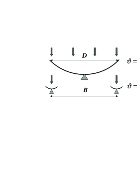
Figure 1: A telescope with aperture diameter $D$ observing at wavelength $\lambda$ has diffraction-limited angular resolution $\theta\simeq\lambda/D$ (upper panel). At the same frequency, a two-element interferometer has an angular resolution along the direction of its baseline $B$, of $\theta\simeq\lambda/B$ (lower panel), equal to the angular resolution of the “single-dish” telescope if $B=D$. Incoming radiation is shown by arrows.

Equations (2) and (3) form the foundation of interferometry and aperture synthesis. Note, that the mutual coherence is a complex function. For convenience, it is usually represented as $\Gamma(u,v)\equiv A(u,v)e^{i2\pi\phi(u,v)}$, where $A(u,v)$ and $\phi(u,v)$ are the amplitude and phase, respectively. In principle, the problem of reconstructing $I(x,y)$ requires a simple inverse Fourier transformation of $\Gamma(u,v)$. However in practice, due to a variety of reasons (telescope-specific instrumental and propagation effects, to mention just a few), the measurement of $\Gamma(u,v)$ is neither complete nor unbiased. The most serious problems surround measurements of the phases of the interferometric response.

3 Closure relations in interferometry

In the early days of radio interferometry, an ingenious method of intensity interferometry had been introduced by Hanbury Brown & Twiss[8] (see also Hanbury Brown[7] and references therein). In this method, the signals from two telescopes were first square-law detected and filtered and then correlated. Problems with measuring phases (as well as accurate synchronization of the receivers at different telescopes) were thus eliminated. As a result, no proper image could be produced, but the output of the correlator was proportional to $<V_{1}V_{2}>^{2}\propto\Gamma(u,v)^{2}$. It was certainly better than nothing as far as the structural properties of the source were concerned. However, the method had a serious disadvantage – a lack of sensitivity. Signal handling by the intensity interferometers requires amplification of the signals before correlation, making the signal-to-noise detection threshold in the incoming data considerably inferior to that of “conventional” interferometers. Nevertheless, this problem did not prevent successful application of intensity interferometry in optical domain (also known as speckle interferometry, see review by Bates[1]).

The intensity interferometry is perhaps worth mentioning here since it resembles some techniques used in detection of particle production and particle interferometry (see Csörgő[5] and references therein).

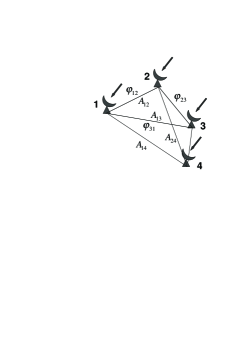
Figure 2: Radio telescopes 1,2,3 and 4 observe a distant celestial source (which is located in the far zone; this allows us to consider the electromagnetic waves shown by arrows as planar waves). Each of the six two-telescope interferometers available in this scheme detect the response represented by its amplitude $A_{ij}$ and phase $\phi_{ij}$ where $i,j=1,2,3,4$. Not all combinations of $A_{ij}$ and $\phi_{ij}$ are shown.

The next breakthrough in interferometry came with the introduction of the so called “closure” relations. First, Jennison[6] conceived the idea of phase closure. It is based on the fact, that in any interferometric triangle, the sum of the three interferometer phases for a point-like source must be zero (see the interferometric triangle “1–2–3” in Fig. 2; the closure phase is $\Phi_{123}\equiv\phi_{12}+\phi_{23}+\phi_{31}$). If any disturbance is imposed on the signal phase generated at an antenna in such the triangle, it will be impressed on the interferometer phase on two baselines linked to that antenna with opposite signs, thus leaving the closure phase unchanged. For a non-point-like source, $\Phi_{123}\neq 0$, but it remains invariant to any telescope-dependent instrumental phase disturbances:

$$\Phi_{123}\equiv\phi_{12}+\phi_{23}+\phi_{31}=\psi_{12}+\psi_{23}+\psi_{31},$$ (4)

where $\psi_{ij}$ are measured (i.e. biased) interferometer phases. The equation (4) is a powerful constraint in recovering true “structural” phases which represent the source structure via equation (3). Note, that baseline-dependent errors cannot be cured by the closure phase relation (4).

Smith[15] and Twiss et al.[17] applied the idea of closure relations to amplitudes. They showed that the value $\mathcal{G}\equiv A_{12}A_{34}/(A_{13}A_{24})$ (dubbed “closure amplitude”; Fig. 2) is independent of the gain (i.e. amplitude) uncertainties.

4 In place of conclusion

This short presentation in no way is a complete description of the broad and versatile technique of interferometry able to study electromagnetic emission of celestial sources with unrivaled angular resolution. Instead, I hope, it can trigger further investigation of possibly deep and potentially fruitful analogies between “classical” interferometry and multiparticle dynamics. It has to be noted that not all possible parallels between the two disciplines have been mentioned here. For example, the idea of correlation of photons produced in W pair production has been suggested earlier by Chapovsky et al.[4].

The following questions seem to be of interest:
1). What is the correspondence (if any) between measurable parameters in astrophysical interferometry and particle dynamics experiments?
2). If the parallel between intensity interferometry and some “correlation” detections in particle collisions is indeed meaningful, what is needed for the particle experiments to be treated as a “conventional” interferometer? The answer on this question could bring about applications of, e.g., closure relations, proven to be extremely valuable in astrophysical interferometry.

In this publication I have chosen not to describe some recent highlights of astrophysical interferometry reviewed in the verbal version of this presentation. Those interested in the state-of-the-art achievements of interferometers in various fields of astrophysics are referred to the recent reviews in the Proceedings of the Symposium “Galaxies and Their Constituents at the Highest Angular Resolution”[14] and references therein.

References

- [1] R.H.T. Bates, Phys. Rep. 90, 203 (1982).
- [2] M. Born & E. Wolf, Principles of Optics, (Pergamon Press, Oxford, 1975).
- [3] W.N. Christiansen & J.A. Warburton, Aust. J. Phys 8, 474 (1955).
- [4] A.P. Chapovsky, V.A. Khoze & W.J. Stirling, Eur. Phys. Jour. C 18, 73 (2000).
- [5] T. Csörgő in Particle Production Spanning MeV to TeV energies, eds. W. Kittel et al., p. 203 (Kluwer, Dordrecht, 2000).
- [6] R.C. Jennison, Mon. Not. Royal Astron. Soc. 118, 276 (1958).
- [7] R. Hanbury Brown, The Intensity Interferometer, (Taylor and Françis, London, 1974).
- [8] R. Hanbury Brown & R.Q. Twiss, Philos. Mag., ser. 7 45, 663 (1954).
- [9] H. Hirabayashi et al., Science 281, 1825 (1998).
- [10] K.I. Kellermann & J.M. Moran, Ann. Rev. Astron. Astroph. (2001).
- [11] P.J. Lena & A. Quirrenbach, Interferometry in Optical Astronomy, Proc. SPIE 4006, (2000).
- [12] A.A. Michelson, Philos. Mag. Ser. 5, 1 (1890).
- [13] M. Ryle & A.Hewish, Mon. Not. Royal Astron. Soc. 120, 220 (1960).
- [14] R.T. Schilizzi, S.N. Vogel, F. Paresce & M.S. Elvis, eds. Galaxies and Their Constituents at the Highest Angular Resolution, Proceedings of the IAU Symposium No. 205, (Astronomical Soc. of the Pacific, 2001).
- [15] F.G. Smith, Proc. Phys. Soc. B 65, 971 (1952).
- [16] A.R. Thompson, J.M. Moran & G.W. Swenson, Interferometry and Synthesis in Radio Astronomy, (Krieger Publ. Co., Malabar, 1998).
- [17] R.Q. Twiss, A.W.L. Carter & A.G. Little, Observatory 80, 153 (1960).