Abstract

An updated analysis of all available neutrino oscillation evidence in Solar experiments including the latest $SNO$ data is presented. Predictions for total rates and day-night asymmetry in Borexino are calculated. Our analysis features the use of exhaustive computation of the neutrino oscillation probabilities and of an improved statistical $\chi^{2}$ treatment.

In the framework of two neutrino oscillations we conclude that the best fit to the data is obtained in the LMA region with parameters $(\Delta m^{2},\tan^{2}\theta)=(5.4\times 10^{-5}\ \mbox{eV}^{2},0.38)$, ($\chi^{2}_{min}/n=0.81$, $n=38$ degrees of freedom). Although less favored, solutions in the LOW and VAC regions are still possible with a reasonable statistical significance. The best possible solution in the SMA region gets a maximum statistical significance as low as $\sim 3\%$.

We study the implications of these results for the prospects of Borexino and the possibility of discriminating between the different solutions. The expected normalized Borexino signal is $0.63$ at the best fit LMA solution, where the DN asymmetry is negligible (approximately $10^{-2}$). In the LOW region the signal is in the range $\sim 0.6-0.7$ at $90\%$ confidence level while the asymmetry is $\simeq 1-20\%$. As a consequence, the combined Borexino measurements of the total event rate with an error below $\pm 5-10\%$ and day-night total rate asymmetry with a precision comparable to the one of SuperKamiokande will have a strong chance of selecting or at least strongly favoring one of the Solar neutrino solutions provided by present data.

$\star$ email: paul@lcm.mi.infn.it, vito.antonelli@mi.infn.it, marco.picariello@mi.infn.it, torrente@cern.ch

1 Introduction

The Solar neutrino problem [1, 2, 3, 4, 5, 6, 7, 8, 9, 10] has been defined, for example, as the difference between the neutrino flux measured by a variety of Solar neutrino experiments and the predictions of the Standard Solar Model (SSM). The explanation of this difference by the neutrino oscillation hypothesis has been boosted by the $SNO$ demonstration at the $3\sigma$ level of the appearance at the Earth of Sun-directed muon and tau neutrino beams [11] and the first determination of the total ⁸B neutrino flux generated by the Sun [12]. The agreement of this flux with the expectations implies as a by-product the confirmation of the validity of the SSM [13, 14, 15].

At present the $SNO$ experiment measures the ⁸B Solar neutrinos via the reactions [16, 17, 18, 19, 19]: 1) Charged Current ($CC$): $\nu_{e}+d\rightarrow 2p+e^{-}$, 2) Elastic Scattering ($ES$): $\nu_{x}+e^{-}\rightarrow\nu_{x}+e^{-}$. The first reaction is sensitive exclusively to electron neutrinos. The second, the same as the one used in SuperKamiokande ($SK$), is instead sensitive, with different efficiencies, to all flavors. The first results by $SNO$ on Solar neutrinos (1169 neutrino events collected during the first 240 days of data, Ref.[12]) confirm previous evidence from $SK$ and other experiments [1, 3, 20, 20, 4]. The Solar neutrino flux measured via the observed CC reaction rate, $\phi_{CC}^{SNO}=1.75\pm 0.07\pm 0.12\times 10^{6}$ cm^-2 $s^{-1}$, is lower than the two existing ES reaction rate measurements: the more precise at $SK$ $\phi_{ES}^{SK}=2.32\pm 0.03\pm 0.08\times 10^{6}$ cm^-2 $s^{-1}$ and the one measured by $SNO$ itself $\phi_{ES}^{SNO}=2.39\pm 0.34\pm 0.15\times 10^{6}$ cm^-2 $s^{-1}$. Comparison of the $\phi_{CC}^{SNO}$ and $\phi_{ES}^{SNO}$ and especially $\phi_{CC}^{SNO}$ and $\phi_{ES}^{SK}$ can be considered as the first direct evidence for Solar neutrino oscillations which cause the appearance of sun-directed muon and tau neutrinos at the Earth. When considering only $SNO$ results, it is advantageous to use the experimental ratio of CC to ES measurements because of the cancellation of systematic errors. The experimental value is

$$R^{\rm exp}=\phi_{CC}^{SNO}/\phi_{ES}^{SNO}=0.748\pm 0.13$$

which is 2$\sigma$ away from the no-oscillation expectation $R^{\rm exp}=1$. Recall that the statistical significance of the difference $\phi_{CC}^{SNO}-\phi_{ES}^{SNO}$ is clearly lower ($\sim 1.4\sigma$) [12]. If we use the $ES$-$SK$ result, the no-oscillation hypothesis is excluded at $\sim 3.3\sigma$ [54, 21, 22]. Moreover the allowed oscillations to only sterile neutrinos is excluded at the same level ($\sim 3\sigma$). Although less favored, the oscillations to both active and sterile neutrinos are still allowed [23, 24, 25, 26, 27, 28, 29].

Although of qualitative importance, the $SNO$ results by themselves, due to their large error bars, are still far from constraining the neutrino oscillation parameters in a significant way. For this purpose we continue to need the data of all other Solar neutrino experiments [1, 2, 4, 30, 31]. The aim of this work is to present an up-to-date analysis of all available Solar neutrino evidence including the latest CC-SNO data in a two-neutrino framework. The predictions for day and night signal rates in the near future real-time ⁷Be sensitive Borexino experiment [32, 33, 34, 35] are also calculated. Two important characteristics of this paper are the use a thorough numerical computation of the neutrino oscillation probabilities and the use of an improved statistical $\chi^{2}$ analysis. The latter is explained in detail in the next section. In summary we have followed the $SK$ standard procedure as close as possible allowing for a better treatment of correlated uncertainties.

As we show below, the best fit to the full data set including global rates and $SK$ energy spectrum is obtained in the Large Mixing Angle (LMA) region. Although less favored, solutions in the Low mass (LOW) and Vacuum (VAC) regions are possible with a reasonable statistical significance. A best fit solution in the Small Mixing Angle (SMA) region is strongly disfavored.

This work is organized as follows. In Section 2 we present a summary of the methods that are used: details of the computation of neutrino oscillation probabilities in the Sun and in the Earth, scattering cross sections and calculation of the signal at the detectors. We continue with a detailed account of the $\chi^{2}$ statistical methods. In Section 3 we present the results of different analyses: first considering total event rates only and then including the $SK$ energy spectrum information. In Section 4 we present our Borexino predictions for the best fit solutions obtained in the previous sections. Finally in Section 5 we summarize and draw conclusions.

2 Methods

2.1 Neutrino oscillations and expected signals

In general, our determination of neutrino oscillations in Solar and Earth matter and of the expected signal in each experiment follows the standard methods found in the literature [36]. Nonetheless, this work differs from previous ones in the treatment of the computation of the neutrino transition probabilities. We completely solve numerically the neutrino equations of evolution for all the oscillation parameter space. Although other alternatives, as the use of semi-analytical expressions in portions of the $(\Delta m^{2},\theta)$ plane, could be previously justified in terms of economy of resources, at this stage a full simulation is an affordable and better option. This is specially true in the calculation of the smearing of the neutrino probability as a function of the neutrino production point when introducing non radial propagation. However no suprises are found: our numerical results are in overall good agreement with the semi-analytical approach.

The survival probabilities for an electron neutrino, produced in the Sun, to arrive at the Earth are calculated in three steps. The propagation from the production point to Sun’s surface is computed numerically in all the parameter range using the electron number density $n_{e}$ given by the BPB2001 model [14] averaging over the production point. The propagation in vacuum from the Sun surface to the Earth is computed analytically. The averaging over the annual variation of the orbit is also exactly performed using simple Bessel functions. To take the Earth matter effects into account, we adopt a spherical model of the Earth density and chemical composition. In this model, the Earth is divided in eleven radial density zones [37], in each of which a polynomial interpolation is used to obtain the electron density. The glueing of the neutrino propagation in the three different regions is performed exactly using an evolution operator formalism [36]. The final survival probabilities are obtained from the corresponding (non-pure) density matrices built from the evolution operators in each of these three regions. The night quantities are obtained using appropriate weights which depend on the neutrino impact parameter and the sagitta distance from neutrino trajectory to the Earth center, for each detector’s geographical location.

The expected signal in each detector is obtained by convoluting neutrino fluxes, oscillation probabilities, neutrino cross sections and detector energy response functions. We have used neutrino-electron elastic cross sections which include radiative corrections [38, 39]. Neutrino cross sections on deuterium needed for the computation of the CC-SNO measurements are taken from [40].

Detector effects are summarized by the respective response functions, obtained by taking into account both the energy resolution and the detector efficiency. The resolution function for CC-SNO is that given in [12]. We obtained the energy resolution function for $SK$ using the data presented in [42, 41, 43]. The effective threshold efficiencies, which take into account the live time for each experimental period, are incorporated into our simulation program. They are obtained from [47].

2.2 The $\chi^{2}$ calculations: definitions and procedures

The statistical significance of the neutrino oscillation hypothesis is tested with a standard $\chi^{2}$ method which we explain in some detail here.

In the most simple case, the analysis of global rates presented in Section 3.1, the definition of the $\chi^{2}$ function is the following:

$$\chi^{2}_{\rm glob} = ({\mbox{\boldmath$R$}^{\rm th}-\mbox{\boldmath$R$}^{\rm exp}})^{T}\left(\sigma^{2}\right)^{-1}({\mbox{\boldmath$R$}^{\rm th}-\mbox{\boldmath$R$}^{\rm exp}})$$ (1)

where $\sigma^{2}$ is the full covariance matrix made up of two terms, $\sigma^{2}=\sigma^{2}_{\rm unc}+\sigma^{2}_{\rm cor}$.

The diagonal matrix $\sigma^{2}_{\rm unc}$ contains the theoretical, statistical and uncorrelated errors while $\sigma^{2}_{\rm cor}$ contains the correlated systematic uncertainties. The ${\mbox{\boldmath$R$}}^{\rm th,exp}$ are vectors containing the theoretical and experimental data normalized to the SSM expectations. The length of these vectors is 3 or 4 depending on whether the CC-SNO experiment is included or not:

$$R^{th,exp}_{i}=S_{i}^{th,exp}/S_{i}^{SSM},\quad i=Cl,\ Ga,\ SK,\ (\mbox{\mbox{ CC-SNO} })\,.$$

The index $i$ denotes the different Solar experiments: Chlorine ($Cl$), Gallium ($Ga$), SuperKamiokande ($SK$) and Charged Current $SNO$ ( CC-SNO ).

The correlation matrices, whether including the $SNO$ experiment or not, have been computed using standard techniques [44, 45].

To test a particular oscillation hypothesis $(\Delta m^{2},\tan^{2}\theta)$ against the parameters of the best fit, we perform a minimization of the $\chi^{2}_{\rm glob}$ as a function of the oscillation parameters. A point in parameter space $(\Delta m^{2},\tan^{2}\theta)$ is allowed if the globally subtracted $\chi_{\rm glob}^{2}$ fulfills the condition $\chi_{\rm glob}^{2}(\Delta m^{2},\theta)-\chi_{\rm min}^{2}<\chi^{2}_{n}(CL)$. Where $\chi^{2}_{n=2}(90\%,95\%,...)=4.60,5.99,...$ are the $n=2$ degrees of freedom quantiles.

A more elaborated statistical analysis is necessary once one introduces the $SK$ energy spectrum into the analysis (Section 3.2).

The procedure assumed by the $SK$ collaboration, in order to present its own analysis and obtain the tables of bin correlated errors, is that of using the summation $\chi^{2}=\sum\chi^{2}_{i}$ where each term is of the form [46, 47]

$$\chi_{i} \sim \alpha\ f_{i}(\delta_{\rm cor})\ R_{i}^{\rm th}-R_{i}^{\rm exp},$$ (2)

and where the expression

$$f_{i}(\delta_{\rm cor}) \sim \frac{1}{1+\sigma_{i,{\rm cor}}\delta_{\rm cor}}$$ (3)

is the response function for the correlated error in the $i^{th}$-energy bin. The $\sigma_{i,{\rm cor}}$ are bin-correlated uncertainties and $\alpha$ is an overall flux normalization factor. The correlation parameter $\delta_{\rm cor}$ is arbitrary and determined in the minimization process together with the rest of oscillation parameters.

SuperKamiokande calculation of tables for correlated errors (as Table III in Ref. [47] and previous publications) and the $\chi^{2}$ prescription given respectively by Eqs. (2) and (3) are closely related. In this work we follow this definition of the $\chi^{2}$, however for clarity we write the expressions in a notation which renders the comparison with other published works simple. It can be easily shown that the expression to be presented below leads to the $SK$ expressions .

Therefore, for the analysis of the full set of data including $SK$ energy spectrum, we consider a $\chi^{2}$ function which is sum of two quantities $\chi^{2}=\chi^{2}_{\rm glob}+\chi^{2}_{\rm spec}$. The first one is given by Eq. (1) considering only $Cl$, $Ga$ and CC-SNO total rates, while for the second term we adopt the definition

$$\chi^{2}_{\rm spec} = \sum_{d,n}({\alpha\mbox{\boldmath$R$}^{\rm th}-\mbox{\boldmath$R$}^{\rm exp}})^{t}\left(\sigma^{2}_{\rm unc}+\delta_{\rm cor}\sigma^{2}_{\rm cor}\right)^{-1}({\alpha\mbox{\boldmath$R$}^{\rm th}-\mbox{\boldmath$R$}^{\rm exp}})+\chi_{\alpha}^{2}+\chi^{2}_{\delta}\,.$$ (4)

A subindex $i=d,n$ corresponding to separated day and night quantities is understood for any $R$ vector and $\sigma$ matrix. We have introduced the flux normalization factor $\alpha$ and the correlation parameter $\delta_{\rm cor}$. The complete variance matrix is not a constant quantity. It is obtained by combining the statistical variances with systematic uncertainties and dependent on this correlation parameter.

The corresponding $\chi^{2}$ terms in Eq. (4) are

$$\chi^{2}_{\alpha}=\frac{\left(\alpha-\alpha^{\rm th}\right)^{2}}{\sigma_{\alpha}^{2}},\quad\chi^{2}_{\delta}=\frac{\left(\delta_{\rm cor}-\delta_{\rm cor}^{\rm th}\right)^{2}}{\sigma_{\delta}^{2}}\,.$$

The central value $\alpha^{\rm th}=1$ corresponds to the BPB 2001 ⁸B flux. The uncertainty on $\alpha$ comes from the ${}^{+19}_{-14}\%$ uncertainty in the ⁸B flux and we make an average of the two-side errors taking $\alpha^{\rm th}\pm\sigma_{\alpha}=1.00\pm 0.17$ [14]. The correlation parameter is assumed to be constrained to vary in a gaussian way with an error corresponding to $\sigma_{\delta}$ and we take $\delta_{\rm cor}^{\rm th}=1$.

In this work we consider two cases. In the first case the flux normalization is taken to be free (we allow for a very large $\sigma_{\alpha}\to\infty$ in the $\chi_{\alpha}^{2}$ term). As a second possibility we consider that both quantities $\alpha$ and $\delta_{\rm cor}$ are constrained. Note that the unwanted consequence of eliminating the last term $\chi^{2}_{\delta}$ would be to obtain running-away solutions for the optimal value of this parameter.

The $\chi^{2}$ summation now contains 41 bins in total: 3 from the global rates (all the experiments except $SK$) and 2$\times$19 bins for the $SK$ day and night spectrums. The full correlation matrix is defined by blocks. The 3$\times$3 block corresponding to the global rates is defined as above. For each day and night spectrum the corresponding 19$\times$19 block correlation matrices are conservatively constructed assuming full correlation among energy bins . The components of the variance matrix are

$$\left(\sigma_{\rm cor}^{2}\right)_{ij} = \sigma_{i,\rm exp}\sigma_{j,\rm exp}+\sigma_{i,\rm cal}\sigma_{j,\rm cal},$$

$$\left(\sigma_{\rm unc}^{2}\right)_{ii} = \sigma_{i,\rm stat}^{2}+\sigma_{i,\rm unc}^{2},$$

where $\sigma_{\rm stat}$ are the statistic errors and the quantities $\sigma_{\rm exp},\sigma_{\rm cal},\sigma_{\rm unc}$ are respectively the bin-correlated experimental, the spectrum calculation uncertainties and the bin-uncorrelated ones.

Notice that in the above sum we do not simultaneously include the global ratio for $SK$ and the partial spectrum bins. We ignore any correlation between the spectrum information and the global rates of all experiments except $SK$ itself. Finally, a remark is in order. In this case the defined covariance matrix is dependent on one of the fitting parameters. One does not, however have to add any correction (i.e. $\log\det\sigma$ terms) to the $\Delta\chi^{2}$ expression as long as we sit at $\delta_{\rm cor}^{\rm min}$. To test a particular oscillation hypothesis and obtain allowed regions in parameter space we perform a minimization of the four dimensional function $\chi^{2}(\Delta m^{2},\tan^{2}\theta,\alpha,\delta_{\rm cor})$. The minimization of the expression with respect to $\alpha$ and $\delta_{\rm cor}$ is done analytically. The subsequent minimization in the $\left(\Delta m^{2},\tan^{2}\theta\right)$ plane is numerical. For $\delta_{\rm cor}=\delta_{\rm cor}^{\rm min},\alpha=\alpha_{\rm min}$, a given point in the oscillation parameter space is allowed if the globally subtracted quantity fulfills the condition $\Delta\chi^{2}=\chi^{2}(\Delta m^{2},\theta)-\chi_{\rm min}^{2}<\chi^{2}_{n}(CL)$. Where $\chi^{2}_{n=4}(90\%,95\%,...)=7.78,9.4,...$ are the quantiles for four degrees of freedom.

3 Results

We have used data on the total event rates measured at chlorine Homestake experiment, at the gallium experiments $SAGE$ [48, 4], $GNO$ [30] and $GALLEX$ [31] and at the water and heavy-water $SK$ (live time 1258 days) [46] and $SNO$ ($ES$,$CC$ 240 days [12]) experiments (see Table (1) for an explicit list of results and references).

For the purposes of this work it is enough to summarize all the gallium experiments in one single quantity by taking the weighted average of their rates.

In addition, for $SK$ we use the available information for the day and night energy spectrums. For each of the day and night cases, this spectrum information contains 18 total recoil-electron energy bins of width 0.5 MeV in the range 5 to 14 MeV and an additional bin spanning the remaining 14-20 MeV range. The data and errors for individual energy bins for $SK$ spectrum has been obtained from Ref. [47]. The information from other $SK$ results as the global day night asymmetry is already contained to a large extent in the previous quantities and does not change the results to be presented on continuation [46, 3].

3.1 Global rate analysis

The analysis of the global rates of the four experiments $SK$, Chlorine, Gallium and CC-SNO is the simplest possibility but nonetheless it reveals important trends of the solutions to the Solar neutrino problem. It illustrates how the CC-SNO data impose additional constraints on the parameter space and in particular how the SMA solution loses its statistical significance in favor of the LMA and LOW regions, becoming allowed only at marginal $\approx 3\sigma$ confidence levels.

We present results both with and without the inclusion of the CC-SNO global rate. In the analysis of the global rates of the $SK$, $Cl$, $Ga$ ( CC-SNO ) experiments one has two free parameters $\Delta m^{2}$ and $\tan^{2}\theta$ and 3 (4) experimental quantities, therefore the effective number of degrees of freedom (d.o.f.) is 1 (2).

On the left-hand-side of Tables (2-3) we present the best fit parameters or local minima obtained from the minimization of the $\chi^{2}$ function given in Eq. (1). Also shown are the values of $\chi^{2}_{\rm min}$ per degree of freedom ($\chi^{2}/n$) and the goodness of fit (g.o.f.) or significance level of each point (definition of SL as in Ref. [49]). On the right-hand-side of the same tables we show the deviations (minimization residuals) from the expected values for all the total event rates. We also include, for further reference, the deviations corresponding to the $SK$ day and night energy spectrums and global day-night asymmetry, although these quantities are not incorporated in the $\chi^{2}$ minimization. We first consider the case in which the CC-SNO global rate is ignored. The absolute minimum is located at the SMA region $(\Delta m^{2},\tan^{2}\theta)^{SMA}=(7.8\times 10^{-6}\ \mbox{eV}^{2},1.10\times 10^{-3})$, with $\chi^{2}_{\rm min}/n=1.06$ (d.o.f. $n=3-2$), the significance level for this point g.o.f. is $29\%$. Closely we find the twin minima situated in the VAC region with parameters $(\Delta m^{2},\tan^{2}\theta)^{VAC}=(8.4\times 10^{-11}\ \mbox{eV}^{2},3.37(0.27))$, which receive a significance level only slightly smaller than the SMA mininimum. The next local minima are situated in the LMA region $(\Delta m^{2},\tan^{2}\theta)^{LMA}=(1.23\times 10^{-5}\ \mbox{eV}^{2},0.34)$, with $\chi^{2}_{\rm min}/n=1.89$ which corresponds to a still reasonable good fit g.o.f. is $17\%$ and in the LOW region $(\Delta m^{2},\tan^{2}\theta)^{LMA}=(1.11\times 10^{-7}\ \mbox{eV}^{2},0.75)$, with $\chi^{2}_{\rm min}/n=3.62$. For comparison, much-less significant results are obtained when sterile neutrino oscillations are considered.

When one introduces the CC-SNO total event rate in the analysis the relative order of the local minima changes. The absolute minimum is now located at the LMA region: $(\Delta m^{2},\tan^{2}\theta)^{LMA}=(3.12\times 10^{-5}\ \mbox{eV}^{2},0.40)$. The significance level of the absolute minimum is clearly worse than in the previous case $\chi^{2}_{min}/n=1.61$ (d.o.f. n=4-2) which corresponds to g.o.f. $=21\%$.

The significance level of the SMA region which follows is no better than $\chi^{2}_{\rm min}/n=2.40$, g.o.f. is $8.8\%$, value which is obtained at $(\Delta m^{2},\tan^{2}\theta)^{SMA}=(7.3\times 10^{-6}\ \mbox{eV}^{2},1.40\times 10^{-3})$. After that, we have the pair of minima at the VAC region $(\Delta m^{2},\tan^{2}\theta)^{VAC}=(9.7\times 10^{-11}\ \mbox{eV}^{2},4.00(0.26))$, with $\chi^{2}_{\rm min}/n=3.2-3.1$. Finally, we find in the table a minimum in the LOW closely situated to the one of the previous case.

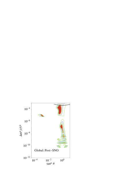
Figure 1: Best fit solutions for the global rate analysis. Global rates from $SK$, $Cl$ and $Ga$ experiments are included. The right figure contains also the CC-SNO one. The black dots are the best fit points (the absolute minimum is located at the SMA (left) or LMA (right) regions). The colored areas are the allowed regions at 90, 95, 99 and 99.7% CL relative to the absolute minimum. The region above the solid line is excluded by $CHOOZ$ results at 99% CL [50].

In Figs. (1) we present graphically our results respectively before and after including the global CC-SNO rate. In the plots one can see the regions which are allowed at 90, 95, 99 and $99.743\%$ confidence levels. The main difference between the plots is an overall reduction of the extent of the allowed area at any CL. The large contiguous areas at 3 and $4\sigma$ which are present along $\tan^{2}\theta\sim 1$ in the first case are converted into well separated patches after the inclusion of $SNO$ results. The most serious consequence is however the considerable reduction on the significance of the SMA region. From the analysis of the four global rates a good part of this region becomes acceptable only at some marginal level. In these and next plots, the region above the line at high $\Delta m^{2}$ is excluded at $99\%$ CL from the negative results of $CHOOZ$ and Palo Verde [50]. Note that regions for very large $\Delta m^{2}\sim 10^{-3}$ eV ² are excluded at the $2-3\,\sigma$ level without need of the $CHOOZ$ result once we included the $SNO$ data.

The reduction of the SMA region can be explained from the tables of deviation (right part in Tables (2-3)). Before the introduction of the CC-SNO global rate in the computation and $\chi^{2}$ minimization the residuals for the CC-SNO data corresponding to the best fit are very high (Table (2)): $2.5\sigma$ for the SMA and also for the LOW solution. The CC-SNO residual values for remaining regions are however smaller. When the CC-SNO data is incorporated into the fit the SMA and LOW regions become less favored. The effect is much more important for the relatively small SMA region. For the LOW region the initial area is large and nearby minima can be found to adjust for the CC-SNO data and still provide reasonable quality fits.

3.2 Day-night $SK$ spectra and global rates

In this section we present the results obtained when including the $SK$ day and night energy spectrum rates in addition to the total event rates of $Cl$, $Ga$ experiments and CC-SNO .

The definition of the $\chi^{2}$ functions and minimization procedures used in the statistical analysis are explained in detail in Section 2.2. The number of experimental data inputs is $2\times 19+3=41$. One now has four free parameters, the oscillation parameters $\Delta m^{2}$ and $\tan^{2}\theta$, the ⁸B neutrino flux normalization factor $\alpha$ and the correlation parameter $\delta_{\rm cor}$. Two cases will be studied. In case A the flux normalization $\alpha$ is considered a free parameter, the number of effective d.o.f. is then $41-4=37$. In case B, the parameter $\alpha$ is constrained to vary around the BPB2001 central value with a standard deviation $\sigma$ given by SSM. We now have $38$ d.o.f.

In Tables (4-5) we present the best fit parameters or local minima obtained from the minimization of the $\chi^{2}$ function given in Eq. (4). As in the previous section, the values of $\chi^{2}_{\rm min}$ per degree of freedom ($\chi^{2}/n$) and the goodness of fit (g.o.f.) or significance level of all minima are shown. In the right part of the tables, the deviations from the expected values or minimization residuals for a number of experimental quantities are listed.

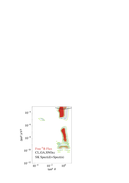
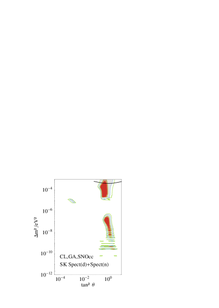
Figure 2: Global solutions for the analysis of $Cl$, $Ga$ and CC-SNO experiments plus the day-night $SK$ spectrum rates. The black dots correspond to best fit points. The colored areas are the allowed regions at 90, 95, 99 and 99.7% CL relative to the absolute minimum. Left (case A of the text): the minimization with respect $\delta_{cor}$ is performed as before. The absolute normalization factor $\alpha$ is allowed to vary freely. Right (case B of the Text): the absolute normalization factor $\alpha$ and correlation parameter $\delta_{\rm cor}$ are varied subject to constraints.

The results for the free flux minimization or case A are presented first. As a summary of numerical results, which appear in detail in Table (4) and Fig. (2, left), the position of the absolute minimum is located at the LMA region $(\Delta m^{2},\tan^{2}\theta)^{LMA}=$ $(5.4\times 10^{-5}\ \mbox{eV}^{2},0.36)$, with $\chi^{2}_{\rm min}/n=0.82$ (d.o.f. n=37). The significance level for this point is noticeably larger (g.o.f. $=82\%$) than the levels obtained in global rates only analysis. This is only in part an artifact of the statistical machinery. It is a satisfactory result because it basically reflects the internal consistency of the data: although the number of degrees of freedom have considerably increased, the $\chi^{2}$ per d.o.f is still much the same. The minimization value of the flux normalization is $\alpha=1.02$ while the correlation parameter is $\delta_{\rm cor}=1.43$. The next local minima are situated at the following positions: the LOW region $(\Delta m^{2},\tan^{2}\theta)^{LOW}=(1.2\times 10^{-7}\ \mbox{eV}^{2},0.75)$, with $\chi^{2}_{min}/n=0.85$ and the two solutions at the VAC region $(\Delta m^{2},\tan^{2}\theta)^{VAC}=(2.7\times 10^{-10}\ \mbox{eV}^{2},2.70(0.32))$, with $\chi^{2}_{\rm min}/n=0.85$. In this last region the best-fit flux normalization is down to $\alpha=0.56$ while $\delta_{\rm cor}=1.65$. In case B, where the flux normalization is constrained to its SSM value, the results are very similar and are shown in Table (5) and Fig. (2, right). The position of the first minimum remains practically unchanged, and is located at the LMA region $(\Delta m^{2},\tan^{2}\theta)^{LMA}=(5.4\times 10^{-5}\ \mbox{eV}^{2},0.38)$, with $\chi^{2}_{\rm min}/n=0.82$ (d.o.f. n=38) and g.o.f.$=82\%$. The next local minima are: the one situated in the LOW region $(\Delta m^{2},\tan^{2}\theta)^{LOW}=(7.5\times 10^{-8}\ \mbox{eV}^{2},0.84)$, with $\chi^{2}_{\rm min}/n=0.86$, and the twin solutions at the VAC region $(\Delta m^{2},\tan^{2}\theta)^{VAC}=(8.9\times 10^{-10}\ \mbox{eV}^{2},1.73(0.48))$, with $\chi^{2}_{\rm min}/n=0.9$. Finally, in both cases A and B we have a local minimum situated at the SMA region. These minima are situated at $\Delta m^{2}\simeq 7.3\times 10^{-6}$ and $\tan^{2}\theta\simeq 1.3\times 10^{-3}$ with a considerable poorer statistical significance.

From the Tables (2-3-4-5) and also from $\chi^{2}$ landscape scans it can be seen that there are some non-negligible regions in parameter space, not only the best fit points. We are therefore justified in converting $\chi^{2}$ into likelihood using the expression ${\cal L}=e^{-\chi^{2}/2}$, and proceeding to study the marginalized parameter constraints. This normalized marginal likelihood is plotted in Figs. (3) for each of the oscillation parameters $\Delta m^{2}$ and $\tan^{2}\theta$. We present results corresponding to two cases: the global-rate analysis excluding CC-SNO and the full analysis including $SK$ energy spectrum. For $\tan^{2}\theta$ we observe that the likelihood function is concentrated in a region $0.2<\tan^{2}\theta<1$ with a clear maximum at $\tan^{2}\theta\sim 0.5$ in sharp coincidence with previous results. The situation for $\Delta m^{2}$ is less obvious although the region at large mass differences is clearly favored. The half width of these curves can be used as another estimate of the minimum error which can be assigned to the parameters at the present and near future experimental situation.

4 Borexino implications

Borexino is a real-time detector for low energy ($<1$ MeV ) spectroscopy. The experiment’s goal is the direct measurement of the ⁷Be Solar neutrino flux of all flavors via neutrino-electron scattering in an ultra-pure scintillation liquid [32, 34, 35, 33].

As before, in order to estimate the Borexino signal one convolutes the Sun-neutrino flux with a detector response function which includes the elastic scattering cross sections $\nu_{e,\mu}e^{-}\rightarrow\nu_{e,\mu}e^{-}$, energy resolution and energy-dependent efficiency effects. We assume a Gaussian resolution function with an energy dependent width $\sigma(E_{exp})=0.048\,\sqrt{E_{exp}}+0.01$ MeV . At this stage we suppose unit efficiency over the nominal window of the experiment $0.3<E<0.8$ MeV and zero otherwise. The absolute ⁷Be flux is taken from BPB2001 [14] as for the other experiments. After one year of data taking, Borexino [55] expects roughly $15-20\times 10^{3}$ Solar neutrino events with a nearly negligible statistical error $\sigma_{stat}\sim 0.8\%$ whereas the error in discriminating signal from background is much larger $\sigma\sim 8\%$ for the same period.

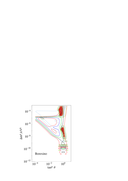
Figure 4: The signal at the Borexino experiment as a function of the oscillation parameters. The signal is normalized to the no-oscillation case. Contours are drawn at $S/S_{0}=0.5,0.6,0.7$ with full lines (respective from inside to outside). Superimposed: the allowed regions from the global rate analysis including CC-SNO (see Fig. (2), right) and the $1\sigma$ allowed regions (here enclosed by the dashed lines) from the ⁸Be sensitive $Cl$ experiment alone.

In Table (6) and Fig. (4) we present the expectations for the normalized day-night signal $S^{day-night}$ at the Borexino experiment for all of the local minima solutions found in the previous section (SK spectrum plus global rates with constrained flux): $S^{Bor}=S^{D-N}(\Delta m^{2},\theta)/S_{0}$ where $S_{0}$ is the expected signal in absence of oscillations and day-night signals are averaged. We also present the expected day-night asymmetry $A^{DN}\equiv 2(D-N)/(D+N)$. As we will see below, the asymmetry on the day-night event rates is a valuable tool for distinguishing among the different oscillation solutions. In Fig. (4) we present the expectations for the Borexino experiment as a function of the two-dimensional oscillation parameters. The expected signal varies mildly in ample regions of the parameter space. We observe that at the best fit solution, situated at the LMA region, the expected Borexino normalized signal is $S^{Bor}=0.63$. In the whole LMA region (99.7% CL) the signal varies between 0.5 and 0.7. If we restrict ourselves to the 90% CL allowed region around the absolute minimum the signal is always within the range $\sim 0.6-0.7$. The asymmetry at the absolute minimum is negligible $A^{DN}<10^{-5}$, while in the LMA region which surrounds it, it can reach the $\sim 1\%$ level. A similar behavior appears in all the rest of the parameter space except in the LOW region.

In the LOW region the signal varies between $\sim 0.6-0.7$ (90% CL). The variation increases to cover the range $\sim 0.5-0.8$ at $99.7$ CL. Here the day-night asymmetry is expected to be at its maximum. From the table one observes values as high as $A^{DN}\simeq 30\%$.

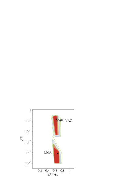
Figure 5: Day night asymmetry $\mid A^{DN}\mid$ versus normalized signal at Borexino corresponding to the 90, 95, 99, 99.7 % CL allowed regions from the full analysis including global rates and SK spectra. The upper (lower) zones correspond to the LOW and VAC (LMA) regions in Fig. (2, left). The stars are the expectations of the best fit solutions in each of the regions.

In the VAC region the signal varies between $\sim 0.7-0.8$. The variation of the expected signal in the SMA region is much more abrupt. This prevents us from giving accurate predictions for this case. The signal passes from a value $S^{Bor}\sim 0.2$ to $S^{Bor}\sim 0.8$ in a very narrow region. As it is shown in Fig. (5), the combined Borexino measurements of the total event rate with an error below $\pm 7-10\%$ and day-night total rate asymmetry with a precision comparable to that of $SK$ will allows us to distinguish or at least to strongly favor the Solar neutrino solutions provided by present data.

5 Conclusions

We have analyzed experimental evidence from all the Solar neutrino data available at this moment including the latest charged current $SNO$ results. For the best solutions which fit the present data, we have obtained and analyzed the expectations in Borexino. We considered different combinations of non-redundant data to perform two kinds of analyses: in the first one we only included total event rates for all the experiments, while in the second we included global rates for $Homestake$, $GNO$-$GALLEX$-$SAGE$ and CC-SNO plus the day and night energy spectrum rates provided by $SK$. In this last case we studied the possibility of free or constrained variations of the Boron Solar neutrino flux.

In the simplest case involving global rates only we have observed how the inclusion of the CC-SNO data causes the strong decrease of the statistical significance of the SMA solution.

In the most comprehensive case, global rates plus spectrum, the best fit was obtained in the LMA region with parameters $(\Delta m^{2},\tan^{2}\theta)^{LMA}=(5.4\times 10^{-5}\ eV^{2},0.38)$, ($\chi^{2}_{\rm min}/n=0.82$, d.o.f. n=38). Solutions in the LOW and VAC regions are still possible although much less favored. The best possible solution in the SMA region gets a low statistical significance.

We have analyzed in detail the expectations on the future experiment Borexino for all the favored neutrino oscillation solutions. The expected Borexino normalized signal is $S^{Bor}=0.63$ at the best-fit LMA solution while the day-night asymmetry is negligible $A^{DN}<10^{-5}$. In the VAC region the signal is slightly higher $\sim 0.7-0.8$ and the asymmetry is still practically negligible. In the whole LMA region (99.7% CL) the signal varies between 0.5 and 0.7. In the LOW region the signal is in the range $\sim 0.6-0.7$ at 90% CL while the asymmetry $A^{DN}\simeq 1-30\%$. We conclude that in the near future, after 2-3 years of data taking, the combined Borexino measurements of the total event rate with an error below $\pm 5-10\%$ and day-night total rate asymmetry with a precision comparable to that of $SK$ will allows us to distinguish or at least to strongly favor the Solar neutrino solutions provided by present data. Additional information and precision measurement should be obtained also from Kamland and from future solar neutrino experiments [56]

Acknowledgments

It is a pleasure to thank R. Ferrari for many enlightening discussions and for his encouraging support without which this work would have not been possible. We thank all the Borexino group of Milano University and especially M. Giammarchi, E. Meroni and B. Caccianiga for providing us essential information about the experiment and its signal discrimination power. One of us (V.A.) would like to thank M. Pallavicini for interesting and useful discussions about Borexino features and potentiality. We thank also all those who sent us comments on early versions of this work. We acknowledge the financial support of the Italian MURST, the Spanish CYCIT funding agencies and the CERN Theoretical Division. The numerical calculations have been performed in the computer farm of the Milano University theoretical group (THEOS).

Experiment [Ref.]	$S_{SSM}$	$S_{Data}/S_{SSM}\ (\pm 1\sigma)$
$SK$ (1258d) [46]	$2.32\pm 0.03\pm 0.08$	$0.451\pm 0.011$
CC-SNO (240d, 8-20 MeV) [12]	$2.39\pm 0.34\pm 0.15$	$0.347\pm 0.029$
$Cl$ [52]	$2.56\pm 0.16\pm 0.16$	$0.332\pm 0.056$
$SAGE$ [4, 48]	$67.2\pm 7.0\pm 3.2$	$0.521\pm 0.067$
$GNO$-$GALLEX$ [30, 31]	$74.1\pm 6.7\pm 3.5$	$0.600\pm 0.067$

Table 1: Summary of data used in this work. The expected signal ($S_{SSM}$) and observed ratios $S_{Data}/S_{SSM}$ with respect to the BPB2001 model are reported. The $SK$ and CC-SNO rates are in $10^{6}$ cm^-2 s^-1 units. The $Cl$, $SAGE$ and $GNO$-$GALLEX$ measurements are in SNU units. In this work we use the combined results of $SAGE$ and $GNO$-$GALLEX$: $S_{Ga}/S_{SSM}$ ($Ga\equiv SAGE$+$GALLEX$+$GNO$)=$0.579\pm 0.050$. The ⁸B total flux is taken from the BPB2001 model [14]: $\phi_{\nu}(\mbox{${}^{8}$B\ })=5.05(1^{+0.20}_{-0.16})\times 10^{6}$ cm^-2 s^-1 .

Solution $\Delta m^{2}$ $\tan^{2}\theta$ $\chi_{m}^{2}/n$ g.o.f.K${}^{K}_{K}$ SMA 7.8 $\times 10^{-6}$ 1.10 $\times 10^{-3}$ 1.1 29 VAC 8.4 $\times 10^{-11}$ 0.27 1.3 26 3.37 1.6 21 LMA 1.2 $\times 10^{-5}$ 0.34 1.9 17 LOW 1.1 $\times 10^{-7}$ 0.75 3.6 5.7

$SK$ $Cl$ $Ga$ $SNO$ $A^{DN}_{SK}$ 0.5 0.8 0.2 2.5 1.3 1.9 1.4 0.8 0.2 1.3 1.7 1.4 0.9 0.3 1.3 0.0 1.3 0.2 0.7 1.1 2.0 1.9 1.0 2.5 0.3

Table 2: (Left) Best fit oscillation parameters: $\Delta m^{2}(\mbox{eV}^{2})$ and $\tan^{2}\theta$, from the analysis of global rates: $Cl$, $Ga$ and $SK$. The $SNO$ measurement is not included (d.o.f.$=3-2$). The significance level g.o.f. is in percentage. The sampling error is $\sim 1\%$ for $\Delta m^{2}$ and $\tan^{2}(\theta)$. (Right) Minimization residuals in 1$\sigma$ units for diverse experimentally measured quantities: the global rates for the four experiments and $SK$ global day-night asymmetry ($A^{DN}$). Only the first three quantities appear in the $\chi^{2}$ computation.

Solution $\Delta m^{2}$ $\tan^{2}\theta$ $\chi_{m}^{2}/n$ g.o.f.K${}^{K}_{K}$ LMA 3.1 $\times 10^{-5}$ 0.40 1.6 21 SMA 7.3 $\times 10^{-6}$ 1.40 $\times 10^{-3}$ 2.4 8.8 VAC 9.7 $\times 10^{-11}$ 0.26 3.1 4.6 4.00 3.2 4.1 LOW 3.2 $\times 10^{-7}$ 0.80 3.3 3.5

$SK$ $Cl$ $Ga$ $SNO$ $A^{DN}_{SK}$ 1.4 0.9 1.5 1.3 1.6 1.0 1.5 0.4 0.9 1.3 3.8 2.3 1.1 1.5 1.3 4.1 2.5 1.3 1.9 1.3 2.7 1.2 3.1 1.7 0.9

Table 3: Best fit oscillation parameters, $\Delta m^{2}(\mbox{eV}^{2})$ and $\tan^{2}\theta$, and minimization residuals (see explanation in Table 2). The analysis now includes the global rates for the four experiments: $Cl$, $Ga$, $SK$ and CC-SNO (d.o.f. $=4-2$).

Solution $\Delta m^{2}$ $\tan^{2}\theta$ $\chi_{m}^{2}/n$ g.o.f.K${}^{K}_{K}$ LMA 5.4 $\times 10^{-5}$ 0.36 0.8 82 LOW 1.2 $\times 10^{-7}$ 0.75 0.8 80 VAC 2.7 $\times 10^{-10}$ 2.70 0.8 80 0.32 0.9 80 SMA 7.3 $\times 10^{-6}$ 1.30 $\times 10^{-3}$ 1.1 40

$SK$ $Cl$ $Ga$ $SNO$ $A^{DN}_{SK}$ 1.8 0.4 0.8 2.1 0.0 2.0 2.0 0.9 2.5 0.2 2.2 1.8 0.5 0.7 1.2 2.3 2.0 0.6 0.8 1.2 0.1 1.0 0.3 2.1 1.3

Table 4: Best fit oscillation parameters, $\Delta m^{2}(\mbox{eV}^{2})$ and $\tan^{2}\theta$, and minimization residuals (see explanation in Table 2). The analysis now includes the global rates for three experiments $Cl$,$Ga$ and CC-SNO , and $SK$ day and night energy spectra. There are four parameters: $\Delta m^{2}$, $\tan^{2}\theta$, $\alpha$ and $\delta_{\rm cor}$. We let the flux normalization $\alpha$ vary freely, so the d.o.f is $=41-4$ (see the text). The sampling error due to the finite-grid is $\sim 1\%$ for $\Delta m^{2}_{min}$ and $\tan^{2}(\theta)$.

Solution $\Delta m^{2}$ $\tan^{2}\theta$ $\chi_{m}^{2}/n$ g.o.f.K${}^{K}_{K}$ LMA 5.4 $\times 10^{-5}$ 0.38 0.8 82 LOW 7.5 $\times 10^{-8}$ 0.84 0.9 72 VAC 8.9 $\times 10^{-10}$ 1.73 0.9 73 0.48 0.9 63 SMA 7.3 $\times 10^{-6}$ 1.30 $\times 10^{-3}$ 1.1 40

$SK$ $Cl$ $Ga$ $SNO$ $A^{DN}_{SK}$ 1.6 0.5 0.9 1.8 0.0 2.7 2.3 0.8 2.9 0.7 2.4 1.9 0.5 0.7 1.3 2.4 2.2 1.4 1.6 1.3 0.1 1.0 0.3 2.1 1.3

Table 5: Same as Table 4 except that here the flux normalization $\alpha$ is constrained to vary with the SSM standard deviation and the d.o.f is $=41-3$ (see the text).

Solution	$\Delta m^{2}(\mbox{eV}^{2})$	$\tan^{2}(\theta)$	$S^{Bor}$	$A^{DN}_{Bor}\ (\%)$
LMA	5.4 $\times 10^{-5}$	0.38	0.63	-0.008
LOW	7.5 $\times 10^{-8}$	0.84	0.61	-14.3
VAC	8.9 $\times 10^{-10}$	1.73	0.64	+0.02
		0.48	0.65	-0.07
SMA	7.3 $\times 10^{-6}$	1.30 $\times 10^{-3}$	0.24	-0.02

Table 6: Borexino experiment expectations for the normalized total signal ($S^{Bor}$) and day-night asymmetry ($A^{DN}$) for all of the best-fit solutions appearing in Table (5).

Figure 3: Marginalized likelihood distributions for each of the oscillation parameters $\Delta m^{2}$ (right), $\tan^{2}\theta$ (left) appearing in the $\chi^{2}$ fit. The curves are in arbitrary units with normalization to the maximum height. The continuous lines shows the distributions corresponding to Fig. (2, right). Dashed lines correspond to the case represented in Fig. (1, left).

References

- [1] R. Davis, Prog. Part. Nucl. Phys. 32 (1994) 13. B.T. Cleveland et al., (HOMESTAKE Coll.) Nucl. Phys. (Proc. Suppl.)B 38 (1995) 47. B.T. Cleveland et al., (HOMESTAKE Coll.) Astrophys. J. 496 (1998) 505-526.
- [2] Y. Fukuda et al. [Super-Kamiokande Collaboration], Phys. Rev. Lett. 82, 2430 (1999) [arXiv:hep-ex/9812011].
- [3] Y. Fukuda et al. [Super-Kamiokande Collaboration], Phys. Rev. Lett. 82, 1810 (1999) [arXiv:hep-ex/9812009].
- [4] J.N. Abdurashitov et al. (SAGE Coll.) Phys. Rev. Lett. 83(23) (1999)4686.
- [5] P. Langacker. Talk given at 4th Intl. Conf. on Physics Beyond the Standard Model, Lake Tahoe, CA, 13-18 Dec. 1994, hep-ph/9503327; Published in Trieste HEP Cosmol.1992:0487-522. Ibid., Nucl. Phys. (Proc. Suppl.)B 77 (1999) 241, hep-ph/9811460. Ibid.., Talk given at 1th Int. Workshop on Weak Interactions and neutrinos (WIN99), Cape Town, SA, 24-30 Jan 1999, hep-ph/9905428.
- [6] P. Ramond, hep-ph/9809401, Nucl. Phys. (Proc. Suppl.)B 77 (1999) 3.
- [7] F. Wilczek, hep-ph/9809509, Nucl. Phys. (Proc. Suppl.)B 77 (1999) 511.
- [8] S.M. Bilenky et al. Summary of the Europhysics neutrino Oscillation Workshop Amsterdam, The Netherlands, 7-9 Sep 1998, hep-ph/9906251. S.M. Bilenky, C. Giunti and C.W. Kim, hep-ph/9902462, Int.J.Mod.Phys.A15(2000) 625.
- [9] E. Torrente-Lujan, arXiv:hep-ph/9902339.
- [10] P. Aliani, V. Antonelli, M. Picariello and E. Torrente-Lujan, arXiv:hep-ph/0112101.
- [11] G. Fiorentini, F. L. Villante, B. Ricci, [arXiv:hep-ph/0109275] .
- [12] Q. R. Ahmad et al. [SNO Collaboration], Phys. Rev. Lett. 87 (2001) 071301 [arXiv:nucl-ex/0106015].
- [13] S. Turck-Chieze, Nucl. Phys. Proc. Suppl. 91 (2001) 73. E. G. Adelberger et al., Rev. Mod. Phys. 70 (1998) 1265 [arXiv:astro-ph/9805121]. A. S. Brun, S. Turck-Chieze and P. Morel, arXiv:astro-ph/9806272.
- [14] J. N. Bahcall, M. H. Pinsonneault and S. Basu, Astrophys. J. 555, 990 (2001) [arXiv:astro-ph/0010346].
- [15] J.N. Bahcall and M.H. Pinsonneault, Rev. Mod. Phys. 67 (1995) 781.
- [16] J. R. Klein [SNO Collaboration], In *Venice 1999, Neutrino telescopes, vol. 1* 115-125. A. B. McDonald [SNO Collaboration], Nucl. Phys. Proc. Suppl. 77 (1999) 43.
- [17] J. Boger et al. [SNO Collaboration], Nucl. Instrum. Meth. A 449 (2000) 172 [arXiv:nucl-ex/9910016].
- [18] V. Barger, D. Marfatia and K. Whisnant, Phys. Lett. B 509 (2001) 19 [arXiv:hep-ph/0104166].
- [19] J. N. Bahcall, P. I. Krastev and A. Y. Smirnov, JHEP 0105 (2001) 015 [arXiv:hep-ph/0103179].
- [20] Y. Fukuda et al. [Super-Kamiokande Collaboration], Phys. Rev. Lett. 81, 1158 (1998) [Erratum-ibid. 81, 4279 (1998)] [arXiv:hep-ex/9805021].
- [21] A. W. Poon [SNO Collaboration], arXiv:nucl-ex/0110005.
- [22] M. V. Garzelli, C. Giunti arXiv:hep-ph/0111254.
- [23] V. Barger, D. Marfatia and K. Whisnant, arXiv:hep-ph/0106207.
- [24] G. L. Fogli, E. Lisi, D. Montanino and A. Palazzo, Phys. Rev. D 64 (2001) 093007 [arXiv:hep-ph/0106247].
- [25] P. I. Krastev and A. Y. Smirnov, arXiv:hep-ph/0108177.
- [26] J. N. Bahcall, M. C. Gonzalez-Garcia and C. Pena-Garay, JHEP 0108, 014 (2001) [arXiv:hep-ph/0106258]; J. N. Bahcall, M. C. Gonzalez-Garcia and C. Pena-Garay, [arXiv:hep-ph/0111150]
- [27] A. Bandyopadhyay, S. Choubey, S. Goswami and K. Kar, arXiv:hep-ph/0110307.
- [28] S. Choubey, S. Goswami and D. P. Roy, arXiv:hep-ph/0109017.
- [29] A. Bandyopadhyay, S. Choubey, S. Goswami and K. Kar, Phys. Lett. B 519 (2001) 83 [arXiv:hep-ph/0106264].
- [30] M. Altmann et al. (GNO Coll.) Phys. Lett. B490 (2000) 16-26.
- [31] P. Anselmann et al., GALLEX Coll., Phys. Lett. B 285 (1992) 376. W. Hampel et al., GALLEX Coll., Phys. Lett. B 388 (1996) 384. T.A. Kirsten, Prog. Part. Nucl. Phys. 40 (1998) 85-99. W. Hampel et al., (GALLEX Coll.) Phys. Lett. B 447 (1999) 127. M. Cribier, Nucl. Phys. (Proc. Suppl.)B 70 (1999) 284. W. Hampel et al., (GALLEX Coll.) Phys. Lett. B 436 (1998) 158. W. Hampel et al., (GALLEX Coll.) Phys. Lett. B 447 (1999) 127.
- [32] T. Hagner [BOREXINO Collaboration], Part. Nucl. Lett. 104, 90 (2001).
- [33] S. M. Bilenky, T. Lachenmaier, W. Potzel and F. von Feilitzsch, arXiv:hep-ph/0109200.
- [34] C. Arpesella et al. [BOREXINO Collaboration], arXiv:hep-ex/0109031.
- [35] E. Meroni, Nucl. Phys. Proc. Suppl. 100, 42 (2001).
- [36] E. Torrente-Lujan, Phys. Rev. D 59 (1999) 093006. E. Torrente-Lujan, Phys. Rev. D 59 (1999) 073001. E. Torrente-Lujan, Phys. Lett. B 441 (1998) 305. V.B. Semikoz, E. Torrente-Lujan, Nucl. Phys. B 556 (1999) 353. E. Torrente-Lujan,Phys. Lett. B494 (2000) 255 [hep-ph/9911458].
- [37] I. Mocioiu and R. Shrock, Phys. Rev. D 62 (2000) 053017 [arXiv:hep-ph/0002149]. A. Dziewonski, in The Encyclopedia of Solid Earth Geophysics, edited by D.E James (Van Nostrand Reinhold, New York 1989).
- [38] J. Bahcall, M. Kamionkowski, A. Sirlin, Phys. Rev. D51 (1995) 6146.
- [39] M. Passera, Phys. Rev. D 64 (2001) 113002 [arXiv:hep-ph/0011190].
- [40] S. Nakamura, T. Sato, V. Gudkov and K. Kubodera, Phys. Rev. C 63 (2001) 034617 [arXiv:nucl-th/0009012].
- [41] H. Ishino, Ph. D. thesis, University of Tokio,1999. M. Nakahata et al. (SK Coll.), Nucl. Instrum. Methods 46 (1998) 301.
- [42] M. Nakahata et al. [Super-Kamiokande Collaboration], Nucl. Instrum. Meth. A 421, 113 (1999) [arXiv:hep-ex/9807027].
- [43] N. Sakurai, Ph.D. Thesis, Dec. 2000 Constraints of the neutrino oscillation parameters from 1117 day observation of soloar neutrino day and night spectra in Super-Kamiokande.
- [44] G. L. Fogli and E. Lisi, Astropart. Phys. 3 (1995) 185.
- [45] S. Goswami, D. Majumdar and A. Raychaudhuri, Phys. Rev. D 63 (2001) 013003 [arXiv:hep-ph/0003163].
- [46] S. Fukuda et al. [Super-Kamiokande Collaboration], Phys. Rev. Lett. 86, 5656 (2001) [arXiv:hep-ex/0103033].
- [47] S. Fukuda et al. [SKamiokande Collaboration], Phys. Rev. Lett. 86, 5651 (2001) [arXiv:hep-ex/0103032].
- [48] A.I. Abazov et al. (SAGE Coll.), Phys. Rev. Lett. 67 (1991) 3332. D.N. Abdurashitov et al. (SAGE Coll.), Phys. Rev. Lett. 77 (1996) 4708. J.N. Abdurashitov et al., (SAGE Coll.), Phys. Rev. C60 (1999) 055801; astro-ph/9907131. J.N. Abdurashitov et al., (SAGE Coll.), Phys. Rev. Lett. 83 (1999) 4686; astro-ph/9907113.
- [49] D. E. Groom et al. [Particle Data Group Collaboration], Eur. Phys. J. C 15 (2000) 1.
- [50] M. Apollonio et al. (CHOOZ coll.), hep-ex/9907037, Phys. Lett. B 466 (1999) 415. M. Apollonio et al., Phys. Lett. B 420 (1998) 397. F. Boehm et al.,Phys. Rev. D62 (2000) 072002 [hep-ex/0003022].
- [51] J. Burguet-Castell and O. Mena, arXiv:hep-ph/0108109.
- [52] K. Lande (For the Homestake Coll.) Nucl. Phys. B(Proc. Suppl.)77(1999)13-19.
-
[53]
J.N. Bahcall, P.I. Krastev and E. Lisi, Phys. Rev. C 55, 494 (1997);
B. Faïd, G.L. Fogli, E. Lisi and D. Montanino, Astropart. Phys. 10, 93 (1999). - [54] V. Berezinsky, arXiv:hep-ph/0108166.
- [55] M. Giammarchi (Borexino Coll.), private communication
- [56] A. Strumia, F. Vissani, JHEP 0111 (2001) 048 [arXiv:hep-ph/0109172] ; A. De Gouvea, C. Peña-Garay, Phys. Rev. D 64 (2001) 113011 [arXiv:hep-ph/0107186] .