AS-ITP-2001-018

Soft Gluon Approach for Diffractive Photoproduction of $J/\psi$

J. P. Ma

Institute of Theoretical Physics , Academia Sinica, Beijing 100080, China

Jia-Sheng Xu

China Center of Advance Science and Technology (World Laboratory), Beijing 100080, China

and Institute of Theoretical Physics , Academia Sinica, Beijing 100080, China

Abstract

We study diffractive photoproduction of $J/\psi$ by taking the charm quark as a heavy quark. A description of nonperturbative effect related to $J/\psi$ can be made by using NRQCD. In the forward region of the kinematics, the interaction between the $c\bar{c}$-pair and the initial hadron is due to exchange of soft gluons. The effect of the exchange can be studied by using the expansion in the inverse of the quark mass $m_{c}$. At the leading order we find that the nonperturbative effect related to the initial hadron is represented by a matrix element of field strength operators, which are separated in the moving direction of $J/\psi$ in the space-time. The S-matrix element is then obtained without using perturbative QCD and the results are not based on any model. Corrections to the results can be systematically added. Keeping the dominant contribution of the S-matrix element in the large energy limit we find that the imaginary part of the S-matrix element is related to the gluon distribution for $x\rightarrow 0$ with a reasonable assumption, the real part can be obtained with another approximation or with dispersion relation. Our approach is different than previous approaches and also our results are different than those in these approaches. The differences are discussed in detail. A comparison with experiment is also made and a qualitative agreement is found.
PACS numbers: 12.38.-t, 12.39.Hg, 13.60.-r, 13.60.Le

Key Words: Soft gluon, HQET, diffractive photoproduction of $J/\psi$, HERA experiment.

1. Introduction

It is usually believed that the nonperturbative QCD plays an important role in diffractive processes and one cannot use perturbative QCD to describe them. Recently it was pointed out[1] that for diffractive production of a vector meson $V$ like

$$\gamma^{*}+h\rightarrow h+V$$ (1)

can be handled with perturbative QCD provided that the virtuality $Q^{2}$ of the initial photon is large. This enables us to make testable predictions for the process and it provides an interesting way to study the nonperturbative nature of the initial hadron, e.g., the structure function of hadrons and of nuclei. For $V=J/\psi$ it is also studied in [2] with perturbative QCD. Theoretically it is proved that the S-matrix element can be factorized[3]. Neglecting higher orders of $Q^{-2}$ the S-matrix element consists of the light-cone wave function of $V$, skewed parton distributions of $h$ and a hard scattering kernel, the hard scattering kernel can be safely calculated with perturbative QCD and it is free from infrared singularities. It should be noted that the factorization also holds if one replaces the vector meson $V$ with a spin-0 meson, or with a photon, the so called deeply virtual Compton scattering[4].

In this work we study the diffractive photoproduction of $J/\psi$

$$\gamma+h\rightarrow h+J/\psi.$$ (2)

Neglecting a possible $c\bar{c}$-content of $h$, the process can be imagined as the following: The photon splits into a $c\bar{c}$-pair, after interactions with the hadron $h$ through gluon exchanges the $c\bar{c}$-pair is formed into $J/\psi$. Because the initial photon is real, i.e., $Q^{2}=0$, the factorization proved in [3] does not apply here. If the total energy is sufficiently large, the exchanged gluons are soft and they can not be handled with perturbative QCD. But the charm quark can be taken as a heavy quark, for emissions of soft gluons by heavy quarks the heavy quark effective theory(HQET) can be used[5], a systematic expansion in the inverse of the charm quark mass $m_{c}$ can be employed to study emissions of soft gluons. Taking the charm quark as a heavy quark it also allows us to use nonrelativistic QCD(NRQCD) to describe nonperturbative properties of $J/\psi$. As an approximation one can take $J/\psi$ as a bound system of a $c$- and $\bar{c}$-quark, in which the $c$- and $\bar{c}$-quark has a momentum which is half of the momentum of $J/\psi$. Corrections to this approximation can be systematically added in the framework of NRQCD[6].

The process studied here has a close similarity to the decay of $J/\psi$

$$J/\psi\rightarrow\gamma^{*}+\pi+\pi\rightarrow e^{+}+e^{-}+\pi+\pi$$ (3)

in the kinematic region where the pions are soft. This decay is studied in [7, 8]. The exchange of soft gluons between the $c\bar{c}$ pair in $J/\psi$ and the pion pair is responsible for the decay. In [7] it is shown that one can use a technique of path integral for the exchange of soft gluons without invoking perturbative QCD. It is also shown that at the leading order of $m_{c}^{-1}$ the decay amplitude derived with the technique of path integral is the same as that derived by assuming that the exchange is of two soft gluons in a special gauge. In this work we will take a suitable gauge and assume the two-gluon exchange in the gauge to derive the S-matrix element for the diffractive process. The assumption can be justified by using HQET: In a suitable gauge the probability for a $c$-quark emitting 1 or 2 gluons is proportional to $m_{c}^{-1}$, while the probability for emission of more than 2 gluons is at order of $m_{c}^{-n}$ with $n>1$. It is interesting to note our result can be derived without taking a suitable gauge and the assumption of two gluon exchange. This can be done with the technique of path integral as that derived for the decay in [7], we briefly sketch how to derive our result in this way and details may be found in [7]. Because the result is derived without the assumption of two gluon exchange in a suitable gauge, our result actually includes effects of exchange of more than 2 gluons in an arbitrary gauge. This will be discussed in detail after our result is represented. The technique of path integral has been used to study exchanges of soft gluons between two light quarks with large momenta[9], where the exchanges were responsible for diffractive scattering of light hadrons.

Our results for the S-matrix element consists of a NRQCD matrix element and a distribution amplitude of gluons in the light hadron $h$. The NRQCD matrix element represents the nonperturbative effect related to $J/\psi$, the distribution amplitude is defined by a matrix element of two field strength operators separated in the moving direction of $J/\psi$ in the space-time. It should be emphasized that the obtained results are not based on any model, corrections to the results can be systematically added in the framework of QCD. At the leading order we consider, the produced $J/\psi$ has the same polarization of the photon, i.e., the produced $J/\psi$ is transversely polarized. In the limit of large beam energies, i.e., $s\rightarrow\infty$, the dominant contribution of the amplitude is related to the skewed gluon distribution of $h$. With a reasonable assumption the forward S-matrix element can be related to the usual gluon distribution $g_{h}(x)$ for $x\rightarrow 0$. This enables us to predict the forward differential cross section with available information of $g_{h}(x)$. With this result it provides an interesting way in experiment to access the small $x$-region of $g_{h}(x)$.

There exist two approaches for the diffractive process in Eq.(1). One is to use perturbative QCD[1, 2], with several approximations one obtains the S-matrix element related to the gluon distribution. Another one is based on the perturbative QCD result for interaction of a small transverse-size dipole of a quark pair, which is formed into $V$. The interaction of the dipole with the initial hadron is through two-gluon exchange[10]. Both approaches have close similarities, In these approaches all hadrons including $J/\psi$ should be taken as massless at the leading order of $Q^{-2}$. Because an expansion in $Q^{-2}$ is used, one can not take the limit $Q^{2}\rightarrow 0$ to obtain predictions for the photoproduction. The expansion in $Q^{-2}$ also implies that the S-matrix element is obtained in the limit of $s\rightarrow\infty$ since $Q^{2}/s$ remains finite. In [11] the approach of the dipole interaction[10] is used, and the effect of the nonzero mass of $J/\psi$ is taken into account. It is found that one can take $Q^{2}\rightarrow 0$ to have the S-matrix element for the photoproduction, where the S-matrix element is also related to the gluon distribution. Similar results are also obtained in [2]. It is questionable if the limit $Q^{2}\rightarrow 0$ can be taken because the higher orders of $Q^{-2}$ are neglected. Our approach is distinctly different. We start directly from the process in Eq.(2) and obtain the S-matrix element for a moderate $s$. Then we take the limit $s\rightarrow\infty$, and the forward S-matrix element in the limit is related to the usual gluon distribution. Our results are also different than those given in [2, 11]. We will discuss the differences in detail.

At first look, one may generalize our results to the case where the initial photon is virtual with a small $Q^{2}$. For transversely polarized $J/\psi$ the generalization is straightforward. But, for longitudinally polarized $J/\psi$ the generalization seems not possible, because the quark mass $m_{c}$ is involved in the polarization vector of $J/\psi$, this can spoil the expansion in $m_{c}^{-1}$. The production of longitudinally polarized $J/\psi$ deserves therefore a further study and we will briefly discuss the problem.

Our work is organized as the following: In Sec. 2. we introduce our notations and derive the S-matrix element in the diffractive region at the leading order of $m_{c}^{-1}$. The result is derived by taking the exchange of two soft gluons in a special gauge into account. We will briefly discuss how to derive it with the technique of path integral. We will also briefly discuss the problem of the $U(1)$ gauge invariance and of the production of longitudinally polarized $J/\psi$. In Sec.3. we derive the forward S-matrix element in the large energy limit. The S-matrix element is related to the usual gluon distribution $g_{h}(x)$ with $x\rightarrow 0$. We discuss the difference between our approach and another approach. In Sec. 4. we compare our results with experiment. Sec.5 is our summary.

2. The soft gluon approach

We consider the process

$$\gamma(k)+h(p)\rightarrow h(p+\Delta)+J/\psi(k-\Delta),$$ (4)

where the momenta are given in the brackets. The Mandelstam variables are defined as

$$s=(k+p)^{2},\ \ \ t=\Delta^{2}.$$ (5)

We study the process in the kinematic region where $|t|$ is at order of $\Lambda_{QCD}^{2}$ and each component of $\Delta$ is at order of $\Lambda_{QCD}$. $h$ is any light hadron whose mass $m$ is at order of $\Lambda_{QCD}$. By taking the charm quark as a heavy quark we have

$$M^{2}_{J/\psi}\gg|t|,\ \ \ s\gg|t|.$$ (6)

It should be noted that we do not require that $s\gg M^{2}_{J/\psi}$, our result presented in this section can be applied to a wide range of $s$. But the value of $s$ should be not too small so that $|t|$ can be small enough. The smallest value of $|t|$ can be approximated by:

$$|t|_{\rm min}=\frac{m^{2}M^{4}_{J/\psi}}{s(s-M^{2}_{J/\psi})}+{\cal O}(\frac{m^{4}}{s})+{\cal O}(\frac{m^{4}}{M^{2}_{J/\psi}}),$$ (7)

hence the value of $s$ should satisfy:

$$s(s-M^{2}_{J/\psi})\gg m^{2}M^{2}_{J/\psi}.$$ (8)

It should be noted that at the threshold we can also have the conditions in Eq.(6), but the exchanged gluons are not soft, hence, our approach presented in this work cannot be used for production at the threshold.

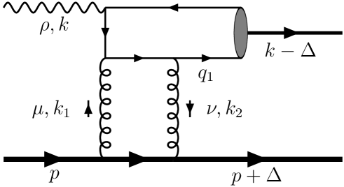
Figure 1: One of six Feynman diagrams for elastic photoproduction of $J/\psi$.

Although our result can be derived exactly by using the technique of path integral as explained in the introduction, we derive here our result by assuming two-gluon exchange in a special gauge, because the derivation in this way is straightforward. We will briefly discuss how to derive our result without the assumption. The contributions of two-gluon exchange to the S-matrix element can be represented by diagrams, one of them is given in Fig.1. The S-matrix element with two-gluon exchange can be obtained directly:

$$\langle f|S|i\rangle = \frac{1}{2}\int d^{4}xd^{4}yd^{4}x_{1}d^{4}x_{2}\int\frac{d^{4}q_{1}}{(2\pi)^{4}}\frac{d^{4}q_{2}}{(2\pi)^{4}}\frac{d^{4}k_{1}}{(2\pi)^{4}}\frac{d^{4}k_{2}}{(2\pi)^{4}}$$ (9)

$$\cdot\varepsilon_{\rho}(k)A_{ij}^{ab,\rho\mu\nu}(k_{1},k_{2},q_{1},q_{2})(2\pi)^{4}\delta^{4}(k+k_{1}-k_{2}-q_{1}-q_{2})$$

$$\cdot e^{-iq_{1}\cdot x-iq_{2}\cdot y}\langle J/\psi|\bar{c}_{i}(x)c_{j}(y)|0\rangle\cdot e^{ik_{1}\cdot x_{1}-ik_{2}\cdot x_{2}}\langle h(p+\Delta)|G^{a}_{\mu}(x_{1})G^{b}_{\nu}(x_{2})|h(p)\rangle,$$

where $\varepsilon(k)$ is the polarization vector of the photon, $c(x)$ is the Dirac field of the $c$-quark, the index $i$ and $j$ stands for color- and Dirac indices. $A_{ij}^{ab,\rho\mu\nu}(k_{1},k_{2},q_{1},q_{2})$ is the scattering amplitude for the process:

$$\gamma(k)+G^{*}(k_{1},a)\rightarrow G^{*}(k_{2},b)+c^{*}(q_{1})+\bar{c}^{*}(q_{2}),$$ (10)

where quarks and gluons are not necessarily on-shell. The matrix $\langle J/\psi|\bar{c}_{i}(x)c_{j}(y)|0\rangle$ represents the nonperturbative effect related to $J/\psi$. It should be noted that for exchange of arbitrary numbers of gluons the same matrix appears in the S-matrix element. Because we take the charm quark as a heavy quark, the $c$- or $\bar{c}$-quark in $J/\psi$ carries roughly the half of the momentum of $J/\psi$, the effect induced by the deviation from the half momentum is suppressed, the suppression parameter is the velocity $v_{c}$ of the $c$- or $\bar{c}$-quark in $J/\psi$ in its rest frame. This fact can be realized by boosting the moving frame of $J/\psi$ to its rest frame, in the rest frame one can then uses NRQCD to perform an expansion in $v_{c}$[6]. We will treat the matrix in the moving frame by using HQET, and then the nonperturbative effect is represented by matrix elements defined in HQET. These matrix elements can be related to those defined in NRQCD. Although the expansion parameter in HQET and in NRQCD is different, but at the orders we consider here this will not cause problems. In this work we take nonrelativistic normalization for heavy quark states and for $J/\psi$ state.

We define the velocity $v$ of $J/\psi$ as

$$v^{\mu}=\frac{(k-\Delta)^{\mu}}{M_{J/\psi}},$$ (11)

the Dirac field $c(x)$ can be expanded in $m_{c}^{-1}$ with fields of HQET:

$$c(x)=e^{-im_{c}v\cdot x}\left\{h(x)+\frac{i}{2m_{c}}\gamma\cdot D_{T}h(x)\right\}+e^{+im_{c}v\cdot x}\left\{g(x)+\frac{i}{2m_{c}}\gamma\cdot D_{T}g(x)\right\}+{\cal O}(m_{c}^{-2}),$$ (12)

where $D_{T}^{\mu}=D^{\mu}-v\cdot Dv^{\mu}$, $D^{\mu}$ is the covariant derivative. $h(x)$ and $g(x)$ are fields of HQET, $h(x)$ can only annihilate a heavy quark and $g(x)$ can only create an heavy antiquark. These fields have the property

$$\gamma\cdot vh(x)=h(x),\ \ \ \gamma\cdot vg(x)=-g(x),$$ (13)

they also depend on the velocity $v$. With these fields the matrix can be written

$$\langle J/\psi|\bar{c}_{i}(x)c_{j}(y)|0\rangle=e^{im_{c}v\cdot(x+y)}\langle J/\psi|\bar{h}_{i}(x)g_{j}(y)|0\rangle+\cdots$$ (14)

where the $\cdots$ stand for higher orders in $m_{c}^{-1}$. With the expansion the $c$- and $\bar{c}$ quark in $J/\psi$ carries the momentum $m_{c}v$ plus some residual momentum, the effect of the residual momentum is represented by the space-time dependence of the matrix element of HQET fields. Because the effect is small, we can neglect the dependence. We obtain:

$$\langle J/\psi|\bar{c}_{i}(x)c_{j}(y)|0\rangle = -\frac{1}{6}e^{im_{c}v\cdot(x+y)}\left[\frac{(1-\gamma\cdot v)}{2}\gamma\cdot\varepsilon^{*}(v)\frac{(1+\gamma\cdot v)}{2}\right]_{ji}\cdot\langle J/\psi|{\bar{h}}\gamma\cdot\varepsilon(v)g|0\rangle$$ (15)

$$+\cdots,$$

where the matrix is diagonal in the color-space, the matrix element is of local fields in HQET, $\varepsilon^{*}(v)$ is the polarization vector of $J/\psi$. We will neglect the higher orders represented by $\cdots$ in the above equations, then the momentum of $J/\psi$ is approximated as $2m_{c}v$. The matrix element $\langle J/\psi|{\bar{h}}(x)\gamma\cdot\varepsilon(v)g|0\rangle$ is related to a NRQCD matrix element defined in the rest frame of $J/\psi$. The relation reads:

$$\sqrt{v^{0}}\langle J/\psi|{\bar{h}}\gamma\cdot\varepsilon(v)g|0\rangle=-\langle J/\psi|\psi^{\dagger}\mbox{\boldmath$\sigma$}\cdot\mbox{\boldmath$\varepsilon$}({\bf v}=0)\chi|0\rangle$$ (16)

where $\psi$ and $\chi$ are NRQCD fields for the $c$- and $\bar{c}$ quark respectively. $\sigma_{i}\ (i=1,2,3)$ is the Pauli matrix. This NRQCD matrix element can be determined from the leptonic decay of $J/\psi$

$$\Gamma(J/\psi\rightarrow e^{+}e^{-})=\alpha_{em}^{2}Q_{c}^{2}\frac{2\pi}{3m_{c}^{2}}|\langle J/\psi|\psi^{\dagger}\mbox{\boldmath$\sigma$}\cdot\mbox{\boldmath$\varepsilon$}({\bf v}=0)\chi|0\rangle|^{2}.$$ (17)

Through examination of contributions of higher orders in Eq.(15) and Eq.(14) one may find that they are suppressed by $v_{c}^{2}$ relatively to the leading order contribution.

With the result in Eq.(15) the S-matrix element reads:

$$\langle f|S|i\rangle = \frac{1}{2}\int d^{4}x_{1}d^{4}x_{2}\int\frac{d^{4}k_{1}}{(2\pi)^{4}}\frac{d^{4}k_{2}}{(2\pi)^{4}}(2\pi)^{4}\delta^{4}(k+k_{1}-k_{2}-2m_{c}v)$$ (18)

$$\cdot(-\frac{1}{6\sqrt{v^{0}}}\langle J/\psi|\psi^{\dagger}\mbox{\boldmath$\sigma$}\cdot\mbox{\boldmath$\varepsilon$}({\bf v}=0)\chi|0\rangle)\cdot(-\frac{i}{2}eQ_{c}g_{s}^{2}\delta_{ab}R^{\mu\nu}(m_{c}v,k_{1},k_{2}))$$

$$\cdot e^{ik_{1}\cdot x_{1}-ik_{2}\cdot x_{2}}\langle h(p+\Delta)|G^{a}_{\mu}(x)G^{b}_{\nu}(y)|h(p)\rangle,$$

where

$$-\frac{i}{2}eQ_{c}g_{s}^{2}\delta_{ab}R^{\mu\nu}(m_{c}v,k_{1},k_{2})={\rm Tr}\left\{\varepsilon_{\rho}(k)A_{ij}^{ab,\rho\mu\nu}(k_{1},k_{2},m_{c}v,m_{c}v)\gamma\cdot\varepsilon^{*}(v)\frac{1+\gamma\cdot v}{2}\right\}.$$ (19)

Now we take the special gauge

$$v\cdot G(x)=0.$$ (20)

In the gauge we have:

$$v_{\mu}G^{\mu\nu}(x)=v_{\mu}\frac{\partial}{\partial x_{\mu}}G^{\nu}(x),$$ (21)

where $G^{\mu\nu}(x)$ is the field strength tensor of gluon. In $R^{\mu\nu}(m_{c}v,k_{1},k_{2})$ $k_{1}$ and $k_{2}$ are the momenta carried by the two exchanged gluons, their components are small in comparison with $m_{c}$, because the two gluons are soft gluons. Hence $R^{\mu\nu}(m_{c}v,k_{1},k_{2})$ can be expanded in $m_{c}^{-1}$, a formal expansion in $m_{c}^{-1}$ leads to:

$$R^{\mu\nu}(m_{c}v,k_{1},k_{2}) = \frac{1}{m_{c}}\cdot\frac{4\varepsilon(k)\cdot\varepsilon^{*}(v)}{v\cdot(k_{1}-k_{2})}\cdot g^{\mu\nu}\cdot\frac{v\cdot k_{1}v\cdot k_{2}}{(v\cdot k_{1}-i0^{+})(v\cdot k_{2}+i0^{+})}+{\cal O}(m_{c}^{-2})$$ (22)

$$+({\rm terms\ proportional\ to\ }v^{\mu}\ {\rm or}\ v^{\nu}),$$

where $0^{+}$ denotes an infinitesimal positive number, which comes from quark propagators. The leading order is $m_{c}^{-1}$. Substituting the result of $R^{\mu\nu}(m_{c}v,k_{1},k_{2})$ at the leading order in the S-matrix element in Eq.(18), the integrations of the components of $k_{1}$, $k_{2}$, $x_{1}$ and $x_{2}$, which are transverse to $v$, can be easily performed, and the result for the S-matrix element at the leading order can be obtained straightforwardly. To present the result we define

$$F_{R}(z) = g_{s}^{2}\int^{\infty}_{-\infty}\frac{d\tau}{2\pi}e^{-i\tau zv\cdot\Delta}v_{\mu}v_{\nu}\langle h(p+\Delta)|G^{a,\mu\rho}(\tau v)G^{a,\nu}_{\ \ \rho}(-\tau v)|h(p)\rangle,$$ (23)

$$\approx g_{s}^{2}\int^{\infty}_{-\infty}\frac{d\tau}{2\pi}e^{i\tau zm_{c}}v_{\mu}v_{\nu}\langle h(p+\Delta)|G^{a,\mu\rho}(\tau v)G^{a,\nu}_{\ \ \rho}(-\tau v)|h(p)\rangle$$

where we have used

$$v\cdot\Delta=-m_{c}\left(1+\frac{t}{4m_{c}^{2}}\right)\approx-m_{c}.$$ (24)

The variable $z$ is related to the momentum $k_{1}$ and $k_{2}$ by

$$v\cdot k_{1}=-\frac{1}{2}v\cdot\Delta(1+z),\ \ \ v\cdot k_{2}=\frac{1}{2}v\cdot\Delta(1-z).$$ (25)

The function $F_{R}(z)$ are zero for $|z|>z_{0}$ with $z_{0}=(2v\cdot p+v\cdot\Delta)/m_{c}$ because of the conservation of momentum. With the function the result for the $S$-matrix element reads:

$$\langle f|S|i\rangle = \frac{2i}{3\sqrt{v^{0}}}eQ_{c}(2\pi)^{4}\delta^{4}(k-\Delta-2m_{c}v)\frac{\varepsilon(k)\cdot\varepsilon^{*}(v)}{m_{c}}$$ (26)

$$\cdot\frac{\langle J/\psi|\psi^{\dagger}\mbox{\boldmath$\sigma$}\cdot\mbox{\boldmath$\varepsilon$}({\bf v}=0)\chi|0\rangle}{(v\cdot\Delta)^{2}}\int dz\frac{1}{(1+z-i0^{+})(1-z-i0^{+})}F_{R}(z)$$

$$\approx \frac{2i}{3\sqrt{v^{0}}}eQ_{c}(2\pi)^{4}\delta^{4}(k-\Delta-2m_{c}v)\frac{\varepsilon(k)\cdot\varepsilon^{*}(v)}{m_{c}^{3}}$$

$$\cdot\langle J/\psi|\psi^{\dagger}\mbox{\boldmath$\sigma$}\cdot\mbox{\boldmath$\varepsilon$}({\bf v}=0)\chi|0\rangle\int dz\frac{1}{(1+z-i0^{+})(1-z-i0^{+})}F_{R}(z).$$

The above results are derived with the assumption of two-gluon exchange in the gauge $v\cdot G=0$. In this gauge the polarization vectors of the two exchanged gluons are perpendicular to $v$. To maintain the color-gauge invariance in other gauges a gauge link must be supplied between the field strength operators in Eq.(23), with the gauge link the effect of exchanges of gluons, whose polarization vectors are proportional to $v$ and whose number is unlimited, is also included. Our result derived in this way may be unsatisfied, because the assumption of two-gluon emission sounds that we performed an expansion in $g_{s}$ for soft-gluons and we add the gauge link by hand. It is possible that the $c\bar{c}$ pair emits soft gluons whose polarizations are all proportional to $v$ and this emission is not suppressed by $m_{c}^{-1}$. This type of contributions was excluded with the gauge. However our result can be derived in an arbitrary gauge without the assumption of two-gluon exchange. The derivation is similar to this for the decay in Eq.(3), we will briefly describe the derivation here, details can be found in [7].

Considering the process with exchange of arbitrary number of gluons in an arbitrary gauge, the matrix element in l.h.s. of Eq.(15) always appears in the S-matrix element. With the approximation in Eq.(15), it is equivalent to consider photoproduction of a $c\bar{c}$-pair, where the $c$- and $\bar{c}$ quark is on-shell and has the same momentum $m_{c}v$. Using the standard SLZ reduction formula we related the $S$-matrix element to Green’s functions, which can be calculated with QCD path integral. Imaging that we perform first the integration over $c$-quark fields, then the problem is formulated as to solve the wave functions of $c$- and $\bar{c}$ quark in the process under a background of gluon fields:

$$\gamma\rightarrow c+\bar{c}.$$ (27)

The background fields vary slowly with the space-time, reflecting the fact that the exchanged gluons are soft. The wave functions can be solved with an expansion in $m_{c}^{-1}$. At leading order, i.e., at order of $m_{c}^{0}$, the wave-functions are obtained by multiplying the wave-functions in the free case with gauge links determined by $v\cdot G$. This means that at the order of $m_{c}^{0}$ only those gluons whose polarization is proportional to $v$, are exchanged. Because of the symmetry of charge conjugation these gauge links do not lead to any physical effect, i.e., the S-matrix element is zero at $m_{c}^{0}$. Solving the wave-functions at order of $m_{c}^{-1}$, one obtains exactly the same results given in Eq.(26), and the gauge link, which needs to be added by hand in Eq.(23), is automatically generated. Because the results are derived without the assumption of two-gluon exchange, they are nonperturbative. The results indicate that the exchange consists of two gluons, whose polarizations are transverse to the moving direction of $J/\psi$, and of any number of gluons, whose polarizations are proportional to $v$.

Our results show that the produced $J/\psi$ is transversally polarized at the order we consider, the production of longitudinally polarized $J/\psi$ is suppressed. As they stand, the results do not respect to the gauge invariance of electromagnetism. This can be seen that the S-matrix element in Eq.(26) is not zero if $\varepsilon(k)$ is replaced by $k$. To study the problem, we note that the performed expansion in $m_{c}^{-1}$ is a formal expansion, the true expansion parameter is $(m_{c}v\cdot k_{1})^{-1}$ or $(m_{c}v\cdot k_{2})^{-1}$, this can also be realized by inspecting the HQET lagrangian. To identify the expansion parameter more clearly, we scale the momenta:

$$k_{1}=\lambda\tilde{k}_{1},\ \ \ k_{2}=\lambda\tilde{k}_{2},$$ (28)

where the components of $\tilde{k}_{1}$ or $\tilde{k}_{2}$ are ${\cal O}(1)$, $\lambda$ is proportional to $\Lambda_{QCD}$ and is small. We note that the $v$-dependence in $R^{\mu\nu}$ appears though $v\cdot k_{1}$ and $v\cdot k_{2}$, if we use $k\cdot\varepsilon(k)=(2m_{c}v+k_{2}-k_{1})\cdot\varepsilon(k)=0$. We scale these factors as:

$$v\cdot k_{1}=m_{c}\tilde{v}\cdot\tilde{k}_{1},\ \ \ v\cdot k_{2}=m_{c}\tilde{v}\cdot\tilde{k}_{2},$$ (29)

where $\tilde{v}\cdot\tilde{k}_{1}$ and $\tilde{v}\cdot\tilde{k}_{2}$ are ${\cal O}(1)$. Now we can expand $R^{\mu\nu}$ in $\lambda$, the result reads:

$$R^{\mu\nu}(m_{c}v,k_{1},k_{2})=\varepsilon_{\rho}w_{1}^{\rho\mu\nu}+{\cal O}(\frac{\lambda}{m_{c}})+({\rm terms\ proportional\ to\ }v^{\mu}\ {\rm or}\ v^{\nu}).$$ (30)

The first term is identical to the term in Eq.(22), which is at order of $\lambda^{0}$, the second term has a length form and is at order of $\lambda$, this implies that the corrections to our results in Eq.(26) is at order of ${\cal O}(\frac{\lambda}{m_{c}})$, where corrections come not only from the term at order of ${\cal O}(\frac{\lambda}{m_{c}})$, but also from emission of more than 2 gluons in the gauge. With this examination the gauge invariance is violated at order of ${\cal O}(\frac{\lambda}{m_{c}})$, i.e., at the next-to-leading order which we neglect, by noting that $k\cdot\varepsilon^{*}(v)={\cal O}(\lambda)$. To restore the gauge invariance, one needs to analyze the contribution at the next-to-leading order. Retaining only the leading order, the gauge invariance holds.

Our results show that the produced $J/\psi$ has the same helicity of the initial photon, i.e., the produced $J/\psi$ is transversally polarized. This is easy to be understood by noting that the exchanged gluons at the considered order do not change the helicity of the $c$- or $\bar{c}$ quark. We can formulate our results as:

$$\langle f|S|i\rangle = (2\pi)^{4}\delta^{4}(k-\Delta-2m_{c}v)\delta_{\lambda_{\gamma}\lambda_{J}}\cdot(-i\frac{2}{3}eQ_{c})\langle J/\psi|\psi^{\dagger}\mbox{\boldmath$\sigma$}\cdot\mbox{\boldmath$\varepsilon$}({\bf v}=0)\chi|0\rangle$$

$$\cdot\frac{1}{\sqrt{v^{0}}m_{c}^{3}}T_{R}\cdot\left\{1+{\cal O}(m_{c}^{-1})+{\cal O}(v_{c}^{2})\right\}$$

$$T_{R} = \int dz\frac{1}{(1+z-i0^{+})(1-z-i0^{+})}F_{R}(z),$$ (31)

where $\lambda_{\gamma}$ and $\lambda_{J}$ is the helicity of the photon and of $J/\psi$, respectively. This is our main result of this section, where the order of errors is also given. The first error is from neglecting higher orders in the $m_{c}^{-1}$ expansion for emission of soft gluons, while the second is from neglecting the relativistic correction related to $J/\Psi$.

If the initial photon is virtual and the virtuality $Q^{2}$ is small, the exchanged gluons are also soft. In this case our approach can be used. It is straightforward to generalize our results to the production of transversally polarized $J/\psi$ with the transversally polarized photon. But, the generalization may not be done for longitudinally polarized $J/\psi$ with longitudinally polarized photon. The reason may be seen from the expansion in $m_{c}^{-1}$ for $R^{\mu\nu}$ in Eq.(22). If the photon and $J/\psi$ are transversally polarized, their polarization vectors have components which are all at order of ${\cal O}(1)$. Then $m_{c}$ is the only large parameter in $R^{\mu\nu}$ and an expansion in $m_{c}^{-1}$ can be performed. This fact is used in the expansion in Eq.(30). If they are longitudinal polarized, their polarization vectors can have components which are very large in comparison with ${\cal O}(1)$, this may prevents us from an expansion in $m_{c}^{-1}$ for $R^{\mu\nu}$. It deserves a further study of the production of longitudinally polarized $J/\psi$.

3. The forward S-matrix element in the limit of $s\rightarrow\infty$

In this section we discuss the S-matrix element in the limit of $s\rightarrow\infty$. In this limit, the function $F_{R}(z)$ can be directly related to the skewed gluon distribution, whose definition can be found in [3, 4]. This can be realized by that in the limit the dominant part of $v$ is proportional to a light cone vector defined below and the correlator defined in Eq.(23) can be expanded with operators classified with twist. The leading order is determined by twist-2 operators. However, the skewed gluon distribution function is not well known and this prevents us from numerical predictions. But, as we will see, there is a possibility to relate the imaginary part of the forward S-matrix element to the usual gluon distribution under certain approximation as in the case of the process in Eq.(1)[1]. We will show that the imaginary part can be related to the gluon distribution with a reasonable assumption and the real part can be estimated by an approximation, then we obtain the forward S-matrix element determined by usual gluon distribution function $g_{h}(x)$ of $h$ for $x\rightarrow 0$. Before taking the limit $s\rightarrow\infty$, we note that the integral over $z$ in $T_{R}$ in Eq.(31) can be performed analytically. Because $F_{R}(z)=0$ for $|z|>z_{0}$, we can extend the integration of $z$ and exchange the integration of $z$ and that of $\tau$ in $F_{R}(z)$. Using an contour integration we obtain:

$$T_{R} = (\pi i)g_{s}^{2}\left\{\int_{0}^{\infty}\frac{d\tau}{2\pi}e^{-i\tau m_{c}}+\int_{-\infty}^{0}\frac{d\tau}{2\pi}e^{+i\tau m_{c}}\right\}v_{\mu}v_{\nu}\langle h(p+\Delta)|G^{a,\mu\rho}(\tau v)G^{a,\nu}_{\ \ \rho}(-\tau v)|h(p)\rangle$$ (32)

$$= (2\pi i)g_{s}^{2}\int_{0}^{\infty}\frac{d\tau}{2\pi}e^{-i\tau m_{c}}v_{\mu}v_{\nu}\langle h(p+\Delta)|G^{a,\mu\rho}(\tau v)G^{a,\nu}_{\ \ \rho}(-\tau v)|h(p)\rangle.$$

For convenience we take a coordinate system in which the photon moves in the $-z$-direction and the hadron $h$ in the $z$-direction. We introduce a light-cone coordinate system, components of a vector $A$ in this coordinate system are related to those in the usual coordinate system as

$$A^{\mu}=\left(A^{+},A^{-},{\bf A_{T}}\right)=\left(\frac{A^{0}+A^{3}}{\sqrt{2}},\frac{A^{0}-A^{3}}{\sqrt{2}},A^{1},A^{2}\right).$$ (33)

The momenta in the process can be approximated in the limit $s\approx 2k^{-}p^{+}\rightarrow\infty$ as:

$$k^{\mu} = (0,k^{-},{\bf 0_{T}}),$$

$$p^{\mu} = (p^{+},\frac{m^{2}}{2p^{+}},{\bf 0_{T}})\approx(p^{+},0,{\bf 0_{T}}),$$

$$\Delta^{\mu} = \left(\frac{t-M_{J/\psi}^{2}}{2k^{-}},\frac{-t-\frac{m^{2}}{p^{+}}\Delta^{+}}{2p^{+}},\mbox{\boldmath$\Delta_{T}$}\right)\approx\left(-\frac{2m_{c}^{2}}{k^{-}},-\frac{t}{2p^{+}},\mbox{\boldmath$\Delta_{T}$}\right)$$

$$v^{\mu} = \frac{(k-\Delta)^{\mu}}{M_{J/\psi}}\approx\left(\frac{m_{c}}{k^{-}},\frac{k^{-}}{2m_{c}},{\bf 0_{T}}\right)\approx\left(0,\frac{k^{-}}{2m_{c}},{\bf 0_{T}}\right),$$ (34)

where $v$ is approximated as a light cone vector. Using these approximated momenta and $M^{2}_{J/\psi}\approx 4m_{c}^{2}\gg|t|$ $T_{R}$ can be written:

$$T_{R}\approx(2\pi i)g_{s}^{2}\frac{k^{-}}{4m_{c}}\int_{0}^{\infty}\frac{d\lambda}{2\pi}e^{-i\lambda x_{c}p^{+}}\langle h(p+\Delta)|G^{a,+\rho}(\frac{\lambda}{2}n)G^{a,+}_{\ \ \ \rho}(-\frac{\lambda}{2}n)|h(p)\rangle,$$ (35)

with

$$n^{\mu}=(0,1,{\bf 0_{T}}),\ \ \ \ x_{c}=\frac{2m_{c}^{2}}{s},$$ (36)

where $T_{R}$ is approximated by the matrix element of the twist-2 operator and corrections can be parameterized with higher-twist operators and they are suppressed by large scales like $s$. We consider the forward case, i.e., $t\rightarrow 0$. For $t\rightarrow 0$ and $\Delta^{\mu}\rightarrow 0$ the integral in Eq.(35) can be approximated by the replacement:

$$\langle h(p+\Delta)|G^{a,+\rho}(\frac{\lambda}{2}n)G^{a,+}_{\ \ \ \rho}(-\frac{\lambda}{2}n)|h(p)\rangle \approx \langle h(p)|G^{a,+\rho}(\frac{\lambda}{2}n)G^{a,+}_{\ \ \ \rho}(-\frac{\lambda}{2}n)|h(p)\rangle=f(\lambda),$$

$$T_{R} \approx (2\pi i)g_{s}^{2}\frac{k^{-}}{4m_{c}}\int_{0}^{\infty}\frac{d\lambda}{2\pi}e^{-i\lambda x_{c}p^{+}}f(\lambda),$$ (37)

with an assumption which we will discuss later in detail. In Eq.(37) we introduce the notation $f(\lambda)$ for the forward matrix element, it has the property $f(\lambda)=f(-\lambda)$. Again, $f(\lambda)$ also appears in the definition of the gluon distribution $g_{h}$ in $h$, in the light cone gauge we use the definition is[13]

$$xg_{h}(x) = -\frac{1}{p^{+}}\int^{\infty}_{-\infty}\frac{d\lambda}{2\pi}e^{-i\lambda p^{+}x}f(\lambda)$$ (38)

$$= -\frac{2}{p^{+}}\int^{\infty}_{0}\frac{d\lambda}{2\pi}\cos(\lambda p^{+}x)f(\lambda).$$

Therefore the forward S-matrix element can be related to the usual gluon distribution. At first look, it seems that there is an ambiguity in relating $T_{R}$ with the usual gluon distribution. One can use the translational covariance to shift the variable $\lambda$ in Eq. (35),

$$\langle h(p+\Delta)|G^{a,+\rho}(\frac{\lambda}{2}n)G^{a,+}_{\ \ \ \rho}(-\frac{\lambda}{2}n)|h(p)\rangle$$

$$=e^{-i\lambda x_{c}p^{+}}\langle h(p+\Delta)|G^{a,+\rho}(0)G^{a,+}_{\ \ \ \rho}(-\lambda n)|h(p)\rangle.$$

If one makes the approximation,

$$\langle h(p+\Delta)|G^{a,+\rho}(0)G^{a,+}_{\ \ \ \rho}(-\lambda n)|h(p)\rangle \approx \langle h(p)|G^{a,+\rho}(0)G^{a,+}_{\ \ \ \rho}(-\lambda n)|h(p)\rangle=f(\lambda),$$

then one will obtain:

$$T_{R}\approx(2\pi i)g_{s}^{2}\frac{k^{-}}{4m_{c}}\int_{0}^{\infty}\frac{d\lambda}{2\pi}e^{-i2\lambda x_{c}p^{+}}f(\lambda),$$ (39)

i.e., one will get a different result, because $x_{c}$ in Eq.(37) is replaced by $2x_{c}$ in Eq.(39) now. This will result in that the forward S-matrix element will be related to the gluon distribution $g_{h}(x)$ at $x=2x_{c}$ instead of $g_{h}(x)$ at $x=x_{c}$, as we will see below in Eq.(41) and Eq.(51). Then we will have two different results of one theory. In the following, we will use the approximation Eq. (37) to derive our results and will demonstrate later that the approximation leading to Eq.(39) is not consistent because some neglected contributions in this approximation are at the same order as those kept in the approximation.

To study the relation of $T_{R}$ to the gluon distribution in detail, we write $T_{R}$ as a sum of the integrals:

$$T_{R}|_{t\rightarrow 0}=\pi ig_{s}^{2}\frac{k^{-}}{4m_{c}}\left\{\int^{\infty}_{-\infty}\frac{d\lambda}{2\pi}+\int^{\infty}_{0}\frac{d\lambda}{2\pi}-\int^{0}_{-\infty}\frac{d\lambda}{2\pi}\right\}e^{-i\lambda p^{+}x_{c}}f(\lambda)$$ (40)

where the first term is simply proportional to the gluon distribution with $x=x_{c}$, the second and third terms can be combined into one integral by using the property $f(\lambda)=f(-\lambda)$:

$$T_{R}|_{t\rightarrow 0}=-i\pi g_{s}^{2}\frac{s}{8m_{c}}\left[xg_{h}(x)\right]|_{x=x_{c}}+\pi g_{s}^{2}\frac{k^{-}}{2m_{c}}\int^{\infty}_{0}\frac{d\lambda}{2\pi}\sin(\lambda p^{+}x_{c})f(\lambda).$$ (41)

In the above equation the first term is the imaginary part of the S-matrix element, the second term is the real part and it can be estimated with dispersion relations. Here we estimate it by another method. We note that the limit $s\rightarrow\infty$ implies $x_{c}\rightarrow 0$, the asymptotic behavior of $g_{h}(x)$ with $x\rightarrow 0$ is expected to be

$$xg_{h}(x)\sim x^{-\alpha},$$ (42)

where $\alpha>0$. With this behavior one can expect that the dominant contribution to the second term is determined by the asymptotic behavior. It is clearly that this behavior is determined by the behavior of $f(\lambda)$ for $\lambda\rightarrow\infty$. For $\lambda\rightarrow\infty$ the function $f(\lambda)$ goes to zero, if $f(\lambda)$ converges to zero fast enough with $\lambda\rightarrow\infty$, the singular behavior in Eq.(42) will not appear. If we calculate $f(\lambda)$ with perturbative theory, the result looks like

$$f(\lambda)|_{\rm pert.}=\lambda^{-2}\left(c_{0}+\sum_{n=1}c_{n}(\ln(\lambda\mu))^{n}\right)+\cdots,$$ (43)

where $\mu$ is the renormalization scale. The terms represented by $\cdots$ will result in singular terms, like $\delta$-functions in the perturbatively calculated gluon distribution. These terms are irrelevant in our case. Neglecting the terms with $\ln(\lambda\mu)$, $f(\lambda)$ behaves like the power behavior $\lambda^{-2}$. However, if one sums all terms with the logarithm $\ln(\lambda\mu)$, the power behavior will be changed. Also nonperturbative effects will definitely change the behavior. We assume that the function $f(\lambda)$ takes the form for $\lambda\rightarrow\infty$:

$$f(\lambda)\approx f_{as}(\lambda)=\frac{a_{g}}{\lambda^{\beta}}$$ (44)

and rewrite the integral in the definition of $g_{h}(x)$ as:

$$xg_{h}(x)=-\frac{2}{p^{+}}\int^{\infty}_{0}\frac{d\lambda}{2\pi}\cos(\lambda p^{+}x)f_{as}(\lambda)-\frac{2}{p^{+}}\int^{\infty}_{0}\frac{d\lambda}{2\pi}\cos(\lambda p^{+}x)(f(\lambda)-f_{as}(\lambda)).$$ (45)

In the second term the function $(f(\lambda)-f_{as}(\lambda))$ will converge to zero faster than $f_{as}(\lambda)$, when $\lambda\rightarrow\infty$, hence the most singular term of $xg_{h}(x)$ for $x\rightarrow 0$ comes from the first term. We write the distribution as:

$$xg_{h}(x)=G_{as}(x)\cdot\left(1+G_{r}(x)\right),\ \ \ G_{as}(x)=\frac{A_{g}}{x^{\alpha}},$$ (46)

where $G_{r}(x)\rightarrow 0$ with $x\rightarrow 0$. It should be noted that in general $G_{r}(x)\cdot G_{as}(x)$ can be singular for $x\rightarrow 0$, $G_{as}(x)$ is the most singular term in $g_{h}(x)$ for $x\rightarrow 0$. With these notations the most singular term in $g_{h}(x)$ is related to $f_{as}(\lambda)$:

$$G_{as}(x) = -\frac{2}{p^{+}}\int^{\infty}_{0}\frac{d\lambda}{2\pi}\cos(\lambda p^{+}x)f_{as}(\lambda)$$ (47)

$$= -\frac{2}{p^{+}}(xp^{+})^{-1+\beta}a_{g}\int^{\infty}_{0}\frac{d\lambda}{2\pi}\lambda^{-\beta}\cos(\lambda).$$

It should be noted that the integral is finite as discussed in the appendix. Comparing with $G_{as}(x)$ in Eq.(47) we obtain the relation between $\alpha$ and $\beta$ and that between $A_{g}$ and $a_{g}$:

$$\alpha = 1-\beta,$$

$$A_{g} = -2(p^{+})^{-2+\beta}a_{g}\int^{\infty}_{0}\frac{d\lambda}{2\pi}\lambda^{-\beta}\cos(\lambda).$$ (48)

With the above discussion we can realize that the dominant contribution to $T_{R}$ is obtained by replacing $f(\lambda)$ with $f_{as}(\lambda)$, and this dominant contribution is determined by the most singular term in the gluon distribution. We will only take this dominant contribution. With the form of $f_{as}(\lambda)$ it is straightforward to calculate $T_{R}$ for $t\rightarrow 0$:

$$T_{R}|_{t\rightarrow 0} \approx (2\pi i)g_{s}^{2}\frac{k^{-}}{4m_{c}}\int_{0}^{\infty}\frac{d\lambda}{2\pi}e^{-i\lambda x_{c}p^{+}}f_{as}(\lambda)$$ (49)

$$= ig_{s}^{2}\frac{k^{-}}{4m_{c}}(x_{c}p^{+})^{-1+\beta}a_{g}\int_{0}^{\infty}{d\lambda}\lambda^{-\beta}\left(\cos(\lambda)-i\sin(\lambda)\right).$$

With the relations in Eq.(48) and results in the appendix for the integrals we obtain:

$$T_{R}|_{t\rightarrow 0}\approx-i\pi g_{s}^{2}\frac{s}{8m_{c}}G_{as}(x_{c})\left[1-i\tan(\frac{1}{2}\alpha\pi)\right].$$ (50)

For a enough small $x_{c}$ one may replace $G_{as}(x_{c})$ with $[x_{c}g_{h}(x_{c})]$ as a good approximation:

$$T_{R}|_{t\rightarrow 0}\approx-\frac{i\pi}{4}g_{s}^{2}m_{c}g_{h}(x_{c})\left[1-i\tan(\frac{1}{2}\alpha\pi)\right].$$ (51)

In the above result the spin of the light hadrons are the same. With the S-matrix element the forward differential cross section reads:

$$\frac{d\sigma}{dt}|_{t\rightarrow 0} = \frac{2}{3\pi s^{2}}\frac{\Gamma(J/\psi\rightarrow e^{+}e^{-})}{\alpha_{em}}\frac{1}{m_{c}^{3}}\overline{\sum}|T_{R}|^{2}$$ (52)

$$\approx \frac{2\pi^{3}\alpha_{s}^{2}}{3}\frac{\Gamma(J/\psi\rightarrow e^{+}e^{-})}{\alpha_{em}m_{c}s^{2}}\left|g_{h}(x_{c})(1-i\tan(\frac{1}{2}\alpha\pi))\right|^{2}$$

where $\overline{\sum}$ is the summation over spin of the final hadron $h$ and the spin average of the initial hadron. This result is our main result in this section. It should be emphasized that we only used the asymptotic behavior of $g_{h}(x)$ to estimate the real part of the amplitude, i.e., the term related to $\tan(\frac{1}{2}\alpha\pi)$, and the imaginary part is determined without using the asymptotic behavior, as it already stands in Eq.(41). With the result in Eq.(51) and Eq.(52) a problem may arise if $\alpha\rightarrow 1$. If $\alpha$ is really close to $1$ or equals to $1$, then the cross section will become infinitely large. However, this can not be the case because $\alpha=1$ implies that the second moment of $g_{h}(x)$, which is the average of the momentum fraction carried by a gluon in the hadron $h$, is infinitely large. Experimentally the extracted second moment is smaller than $1$. The value of $\alpha$ from different parameterization of $g_{h}$ , relevant to our case, is found to be $0.15\sim 0.35$ for $J/\psi$, the corresponding value for $\Upsilon$ production is $0.30\sim 0.48$.

Now we are in the position to discuss the assumption leading to the approximation in Eq.(37) and the mentioned ambiguity. After the integration over $z$ in Eq.(34) we have neglected the $i0^{+}$. Keeping this term the result reads:

$$T_{R}\approx(2\pi i)g_{s}^{2}\frac{k^{-}}{4m_{c}}\int_{0}^{\infty}\frac{d\lambda}{2\pi}e^{-i\lambda x_{c}p^{+}-0^{+}\lambda}\langle h(p+\Delta)|G^{a,+\rho}(\frac{\lambda}{2}n)G^{a,+}_{\ \ \ \rho}(-\frac{\lambda}{2}n)|h(p)\rangle.$$ (53)

With this term we can expand the matrix element in $\lambda$ and perform the integration over $\lambda$ analytically. The result is:

$$T_{R}\approx\pi g_{s}^{2}\frac{s}{4m_{c}}\sum_{n=0}^{\infty}\frac{1}{(x_{c}-i0^{+})^{2n+1}}\frac{\langle h(p+\Delta)|O_{2n+2}|h(p)\rangle}{(p^{+})^{2n+2}},$$ (54)

where operators $O_{J}$ with $J=2,4,6,\cdots$ are the standard twist-2 operators in the light-cone gauge:

$$O_{J}=G^{a,+\mu}\left(\frac{i}{2}\raisebox{7.74998pt}{\leavevmode\hbox{\makebox[0.0pt][l]{${\scriptstyle\leftharpoonup}$}{${\scriptstyle\rightharpoonup}$}}}\partial^{+}\right)^{J-2}G^{a,+}_{\ \ \ \mu},\ \ \ \ J=2,4,6,\cdots,$$ (55)

and the $J$-th moment $a_{J}$ of gluon distribution function is then given by:

$$\langle h(p)|O_{J}|h(p)\rangle=(p^{+})^{J}a_{J}.$$ (56)

In the following discussion we neglect the spin-flip terms, these terms can be discussed in the same way and they do not contribute at the leading order.

In the limit $s\gg 4m_{c}^{2}\gg t$ we can first neglect the $t$-dependence of matrix elements and only keep the dependence of $p^{+}$ and of $\Delta^{+}$. For $\Delta^{+}\rightarrow 0$ the matrix elements can be expanded as:

$$\frac{\langle h(p+\Delta)|O_{2n+2}|h(p)\rangle}{(p^{+})^{2n+2}}=a_{2n+2}+\sum_{k=1}^{\infty}(\frac{-\Delta^{+}}{2p^{+}})^{k}b_{2n+2,k}=a_{2n+2}+\sum_{k=1}^{\infty}x_{c}^{k}b_{2n+2,k},$$ (57)

using these expansions we obtain

$$T_{R}\approx\pi g_{s}^{2}\frac{s}{4m_{c}}\left\{\sum_{n=0}^{\infty}\frac{1}{(x_{c}-i0^{+})^{2n+1}}a_{2n+2}+\sum_{k=1}^{\infty}x_{c}^{k}\sum_{n=0}^{\infty}\frac{1}{(x_{c}-i0^{+})^{2n+1}}b_{2n+2,k}\right\}.$$ (58)

If we assume that for $n\rightarrow\infty$ the behavior of $b_{2n+2,k}$ is similar as $a_{2n+2}$ or $b_{2n+2,k}$ converges faster than $a_{2n+2}$, then the dominant contribution for small $x_{c}$ comes from the first sum, i.e., the dominant contribution comes from the terms with the moments $a_{J}$ of the gluon distribution, and other sums with $b_{2n+2,k}$ are suppressed by positive powers of $x_{c}$. The first sum can be written as a integration from, which is just the approximation used in Eq.(37). Now we consider the approximation in Eq.(39). Using translational covariance the integral can be written:

$$T_{R}\approx(2\pi i)g_{s}^{2}\frac{k^{-}}{4m_{c}}\int_{0}^{\infty}\frac{d\lambda}{2\pi}e^{-i2\lambda x_{c}p^{+}-0^{+}\lambda}\langle h(p+\Delta)|G^{a,+\rho}(0)G^{a,+}_{\ \ \rho}(-\lambda n)|h(p)\rangle.$$ (59)

Similarly, the integral can be written as a sum:

$$T_{R}\approx\pi g_{s}^{2}\frac{s}{4m_{c}}\sum_{n=0}^{\infty}\frac{1}{(2x_{c}-i0^{+})^{n+1}}\frac{\langle h(p+\Delta)|G^{a,+\mu}(i\partial^{+})^{n}G^{a,+}_{\ \ \ \mu}|h(p)\rangle}{(p^{+})^{n+2}}.$$ (60)

We divide the sum into a parts with even $n$ and another part with odd $n$:

$$T_{R} \approx \pi g_{s}^{2}\frac{s}{4m_{c}}\sum_{k=0}^{\infty}\frac{1}{(2x_{c}-i0^{+})^{2k+1}}\frac{\langle h(p+\Delta)|G^{a,+\mu}(i\partial^{+})^{2k}G^{a,+}_{\ \ \ \mu}|h(p)\rangle}{(p^{+})^{2k+2}}$$ (61)

$$+\pi g_{s}^{2}\frac{s}{4m_{c}}\sum_{k=0}^{\infty}\frac{1}{(2x_{c}-i0^{+})^{2k+2}}\frac{\langle h(p+\Delta)|G^{a,+\mu}(i\partial^{+})^{2k+1}G^{a,+}_{\ \ \ \mu}|h(p)\rangle}{(p^{+})^{2k+3}}.$$

For $\Delta^{+}\rightarrow 0$ the matrix elements behave like:

$$\frac{\langle h(p+\Delta)|G^{a,+\mu}(i\partial^{+})^{2k}G^{a,+}_{\ \ \ \mu}|h(p)\rangle}{(p^{+})^{2k+2}} = a_{2k+2}+{\cal O}(\frac{\Delta^{+}}{p^{+}}),$$

$$\frac{\langle h(p+\Delta)|G^{a,+\mu}(i\partial^{+})^{2k+1}G^{a,+}_{\ \ \ \mu}|h(p)\rangle}{(p^{+})^{2k+3}} = -(2k+1)\frac{\Delta^{+}}{2p^{+}}a_{2k+2}+{\cal O}((\frac{\Delta^{+}}{p^{+}})^{2})$$ (62)

$$= (2k+1)x_{c}a_{2k+2}+{\cal O}(x_{c}^{2})$$

From these one would neglect the matrix elements with odd numbers of derivatives, i.e., one would neglect the summation in the second line of Eq.(61), because the matrix elements with odd numbers of derivatives go to zero with $\Delta^{+}\rightarrow 0$, or with $x_{c}\rightarrow 0$ by noting $\Delta^{+}=-2x_{c}p^{+}$. Keeping only the leading terms of the matrix elements with even numbers of derivatives and neglecting the matrix elements with odd numbers of derivatives, one obtains:

$$T_{R}\approx\pi g_{s}^{2}\frac{s}{4m_{c}}\sum_{k=0}^{\infty}\frac{1}{(2x_{c}-i0^{+})^{2k+1}}a_{2k+1}.$$

Writing the sum into a integration form as done for Eq.(58), one obtains the approximation in Eq.(39) and we will get the result for $T_{R}$ which is related to $g_{h}(x)$ with $x=2x_{c}=4m_{c}^{2}/s$. But, the matrix elements with odd numbers of derivatives in the second line in Eq.(61) can not be neglected. Although they are proportional to $x_{c}$ as $x_{c}\rightarrow 0$, but the power of $x_{c}$ in the denominator in the second sum is $2k+2$ in comparison with the power $2k+1$ in the sum of the first line. Keeping the leading terms for matrix elements with even numbers and odd numbers of derivatives, one obtains

$$T_{R}\approx\pi g_{s}^{2}\frac{s}{4m_{c}}\sum_{k=0}^{\infty}\frac{1}{(2x_{c}-i0^{+})^{2k+1}}\cdot a_{2k+1}+\pi g_{s}^{2}\frac{s}{8m_{c}}\sum_{k=0}^{\infty}\frac{(2k+1)}{(2x_{c}-i0^{+})^{2k+1}}a_{2k+1}.$$

Clearly both sums give equally important contributions to $T_{R}$. Actually every term in the expansion in $\Delta^{+}$ for matrix elements with odd numbers of derivatives can lead to a equally important contribution to $T_{R}$. To sum the leading order contributions one can use

$$\langle h(p+\Delta)|G^{a,+\mu}(\partial^{+})^{n}G^{a,+}_{\ \ \ \mu}|h(p)\rangle=\sum_{k=0}^{n}\frac{n!}{k!(n-k)!}(\frac{i\Delta^{+}}{2})^{k}\langle h(p+\Delta)|G^{a,+\mu}\left(\frac{1}{2}\raisebox{7.74998pt}{\leavevmode\hbox{\makebox[0.0pt][l]{${\scriptstyle\leftharpoonup}$}{${\scriptstyle\rightharpoonup}$}}}\partial^{+}\right)^{n-k}G^{a,+}_{\ \ \ \mu}|h(p)\rangle$$ (63)

to re-arrange the sum. With the same assumption made after Eq.(58) one will get the same result as that obtained with the approximation in Eq.(37).

In this section we neglect corrections suppressed by the inverse of $s$ in the limit $s\rightarrow\infty$ and use two assumptions to derive our results in Eq.(51) and Eq.(52): One is used in Eq.(37) and specified in detail between Eq.(58) and Eq.(59), another is to use the assumed asymptotic behavior to determine the real part of the S-matrix element. Without these two assumptions one can relate $F_{R}(z)$ in the limit to the skewed gluon distribution by neglecting corrections suppressed by the inverse of $s$. The relation reads:

$$F_{R}(z)\approx-g_{s}^{2}\frac{s}{8m_{c}}x_{1}x_{2}f_{g}(x_{1},x_{2}),$$ (64)

where we used the definition of skewed parton distributions in [3]. There exists different definitions and the relation between them is well discussed in [14]. The variables $x_{1}$ and $x_{2}$ are related to $z$ as:

$$x_{1}=\frac{2m_{c}^{2}}{s}(1-z),\ \ \ \ \ \ x_{2}=-\frac{2m_{c}^{2}}{s}(1+z).$$ (65)

With this we end up with the result for $T_{R}$:

$$T_{R}\approx-\frac{g_{s}^{2}m_{c}}{4}\int dx_{2}\frac{1}{(x_{1}-i0^{+})(x_{2}+i0^{+})}x_{1}x_{2}f_{g}(x_{1},x_{2}),$$ (66)

with

$$x_{1}-x_{2}=\frac{4m_{c}^{2}}{s}.$$ (67)

Without any knowledge about $f_{g}(x_{1},x_{2})$, the integral can not be performed and numerical predictions can not be made.

With our results we are in position to compare our result with others obtained in [11]. The starting point there is to consider the process in Eq.(1), where the initial photon is virtual. The interaction between the initial hadron $h$ and the $c\bar{c}$ pair is taken as that between $h$ and a $c\bar{c}$ dipole with a small transverse-size. Using the perturbative result, in which only the exchange of two gluons are considered, one obtains at the leading order of $Q^{-2}$:

$$\frac{d\sigma}{dt}|_{t\rightarrow 0}\sim\frac{1}{(Q^{2})^{4}}|(1+i\beta_{s})\left[xg_{h}(x)\right]|^{2}\left\{1+{\cal O}(Q^{-2})\right\},\ \ \ \ {\rm with}\ x=\frac{Q^{2}}{s}.$$ (68)

To derive the result one uses a light-cone wave function to describe the nonperturbative properties of $J/\psi$ and $J/\psi$ should be taken as massless to consistently perform the expansion in $Q^{-2}$. In the above equation the terms relevant for our comparison are given explicitly. As also pointed in [1], the leading log approximations in $\ln(1/x)$ and in $\ln(Q^{2}/\Lambda^{2}_{QCD})$ are required to identify the quantity $x=Q^{2}/s$ as the variable of the gluon distribution $g_{h}(x)$. The produced $J/\psi$ is longitudinally polarized. It should be noted that by taking the $c\bar{c}$ pair as a small dipole it is equivalent to neglect higher orders in $Q^{-2}$[11]. To include the production of a transversally polarized $J/\psi$, the above result is re-derived by keeping the mass $M_{J/\psi}$ and it is found that at leading order of $Q^{-2}$ the result is obtained by replacing $Q^{2}$ with $Q^{2}+M^{2}_{J/\psi}$. The results for the production of $J/\psi$ with a real photon are obtained simply by taking $Q^{2}\rightarrow 0$ in the above result, after the replacement of $Q^{2}$ with $Q^{2}+M^{2}_{J/\psi}$[11, 12]. Several modifications of the results are then introduced, and the relation between the forward S-matrix element and the gluon distribution becomes complicated. We will compare the result in [2, 11, 12] without these modifications. The result in [11, 12] by taking $Q^{2}\rightarrow 0$ is:

$$\frac{d\sigma}{dt}|_{t\rightarrow 0}\sim\frac{1}{(4m^{2}_{c})^{4}}|(1+i\beta_{s})\left[xg_{h}(x)\right]|^{2},\ \ \ \ {\rm with}\ x=\frac{4m_{c}^{2}}{s},$$ (69)

where the term with $\beta_{s}$ is the real part of the amplitude and is given by:

$$i\beta_{s}\left[xg_{h}(x)\right]\approx i\frac{\pi}{2}\frac{\partial xg_{h}(x)}{\partial\ln x}.$$ (70)

If we take $\alpha$ in Eq.(42) as a small parameter, this part is the same as ours. The main difference between our result and that given above is that the S-matrix element is related to the gluon distribution $g_{h}(x)$ at different $x$. It is possible that the limit $Q^{2}\rightarrow 0$ can not be taken because higher orders in $Q^{-2}$ are neglected in Eq.(68).

Similar derivation of the results by using a nonrelativistic wave-function for $J/\psi$ is also done in [2, 15], by keeping the mass of $J/\psi$ at the leading order of $Q^{-2}$ and neglecting higher orders in $Q^{-2}$. Setting $Q^{2}=0$ one obtains:

$$\frac{d\sigma}{dt}|_{t\rightarrow 0}\approx\frac{16\pi^{3}\alpha_{s}^{2}}{3}\frac{\Gamma(J/\psi\rightarrow e^{+}e^{-})}{\alpha_{em}M^{5}_{J/\psi}}\left(2x_{c}g_{h}(2x_{c})\right)^{2}.$$ (71)

This result looks similar as ours, but the differential cross section is related to $xg_{h}(x)$ at $x=2x_{c}$ as the result in Eq.(69) and the real part of the amplitude is neglected.

4. Comparison with experiment

In this section we will compare our results with experiment performed at HERA. In the last two sections we have given our results, but not specified the energy scale $\mu$, at which the nonperturbative quantities like the gluon distribution are defined. To compare with experiment one must choose this scale. In general one may take the scale $\mu$ as a soft scale at order of $\Lambda_{QCD}$ because of the emission of soft gluons. If one takes $\mu$ as a soft scale, then the scale should be the same in the production of $\Upsilon$. However, there can be exchanges of hard gluons between quark lines, between gluon lines and between quark- and gluon lines. The effect can be studied with perturbative QCD and log terms like $\ln(\mu/m_{c})$ appear, one may then identify the scale $\mu$ as $m_{c}$ for $J/\psi$ and as $m_{b}$ for $\Upsilon$, respectively. We will compare our results with experiment with these two choices. It should be pointed out that significant corrections to our results for $J/\psi$ exist, as discussed below. Before these corrections are under control, a detailed comparison of theoretical results with experiment can not be made. In this section we only give numerical results based on our results at leading orders without any modifications, suggested by those corrections.

To predict the total cross section we assume that

$$\frac{d\sigma}{dt}(t)=\frac{d\sigma}{dt}(t=0)e^{-B|t|},$$ (72)

where the slope parameter $B$ is measured as $B\approx 4.5{\rm GeV}^{-2}$[16]. If the scale $\mu$ is taken as a soft scale, there is no detailed information available for the gluon distribution at the scale, one may know that $xg_{h}(x)$ is divergent like $x^{-\alpha}$ when $x\rightarrow 0$. Then the cross section behaves like:

$$\sigma(J/\psi)=A\left(\frac{W_{\gamma p}}{W_{0}}\right)^{\delta},\ \ \ \ W_{0}=1{\rm GeV},$$ (73)

where $W_{\gamma p}=\sqrt{s}$ and $\delta=4\alpha$. If we assume that the parameter $B$ is the same for $\Upsilon$, then we can predict the cross section of $\Upsilon$ by determining the parameters in Eq.(73) from experimental data for $J/\psi$[16]. This can also be considered as we neglect the $\mu$-dependence. We fit the published HERA data with Eq.(73) and obtain:

$$\delta=0.83\pm 0.13,\ \ \ \ \,A=1.37\pm 0.84{\rm nb},\ \ \ \ \ \chi^{2}/d.o.f.=0.31.$$ (74)

The fitting quality is quite good indicated by the small value of $\chi^{2}/d.o.f.$. The fitting cure with experimental data is also shown in Fig. 2. With the determined parameters we can predict:

$$\sigma(\Upsilon) \approx 2.7\times 10^{-2}~{}{\rm nb},\ \ \ \,{\rm for}\ W_{\gamma p}=120~{}{\rm GeV},$$

$$\sigma(\Upsilon) \approx 3.2\times 10^{-2}~{}{\rm nb},\ \ \ \,{\rm for}\ W_{\gamma p}=143~{}{\rm GeV}.$$ (75)

However these predicted values are too small in comparison with the central values of experimental results shown in Fig. 4. Different reasons are responsible for this discrepancy. Firstly we note that there are large errors in experimental data, even large errors in determining the energy $W_{\gamma p}$. Secondly, there are several uncertainties in our predictions, e.g., relativistic corrections arising in the expansion in Eq.(12), corrections from higher orders in the expansion in $m_{c}^{-1}$, and also the leading order determination of the matrix element through the leptonic decay in Eq.(17), etc.. Among them the effects from relativistic corrections and from the determination of the matrix element can be most significant. Because the $c$- or $\bar{c}$ quark moves in the $J/\psi$ rest frame with the velocity $v_{c}$, which is not very small, indicated by $v_{c}^{2}\approx 0.3$, the relativistic correction can be significant. In our approach this correction can be systematically added and its study is underway. In the determination of the matrix element we have used the leading order result for the leptonic decay in Eq.(17). It is well known that the corrections from higher orders in $\alpha_{s}$ are large[17, 18]. Also, the relativistic correction to the result is significant[19]. It is clear that without these corrections an accurate prediction can not be made for the production of $J/\psi$. For the production of $\Upsilon$ these corrections are expected to be small.

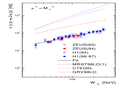
Figure 2: The cross section of elastic photoproduction of $J/\psi$ versus $W_{\gamma p}$, the photon-proton center-of-mass energy. The data points are published HERA results[16]. The full solid line represents a fit of the form $\sigma(J/\psi)\propto W_{\gamma p}^{\delta}$. The theoretical predictions of present work using various parameterizations of the leading gluon density in the proton at $m_{c}$ scale are also shown.

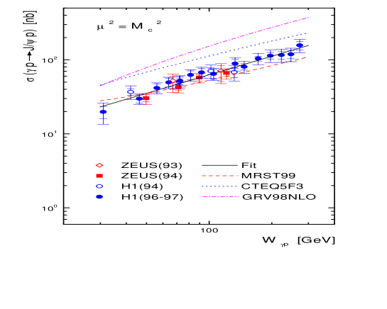
Figure 3: The cross section of elastic photoproduction of $J/\psi$ versus $W_{\gamma p}$, the photon-proton center-of-mass energy. The data points are published HERA results[16]. The full solid line represents a fit of the form $\sigma(J/\psi)\propto W_{\gamma p}^{\delta}$. The theoretical predictions of present work using various parameterizations of the next-to-leading gluon density in the proton at $m_{c}$ scale are also shown.

If we take the scale $\mu$ as the heavy quark mass, we can predict cross sections without any input parameter, because the gluon distribution at the scale is determined. We use the recently determined sets of parton distributions GRV98[20], CTEQ5[21], MRST99[22] and MRST98LO[23]. We do not use the newest MRST01 distributions for $J/\psi$, because it has an unphysical zero at $\mu=m_{c}$ in the gluon distribution and for small $x$ the distribution turns to be negative[24]. Instead we use an old set of parton distributions[22]. The predictions with experimental data[16] are also shown in Fig.2 with leading order gluon distribution, and in Fig.3 with the next-to-leading order gluon distribution. With these distributions we can determine the contribution of the real part of the S-matrix element to the cross section. The contribution is at $12\%$-, $20\%$- and $26\%$ level with the leading order gluon distribution of MRST98LO, CTEQ5L and GRV98LO, respectively, while with the next-to-leading order gluon distribution of MRST99, CTEQF3 and GRV98 it is at $6\%$-, $8\%$- and $12\%$ level, respectively. From these figures we can see that all distributions give the results roughly with the same feature that the cross section increases with the energy, numerical results with the next-to-leading distribution of MRST99 are close to the experimental results for large $s$, while the prediction with other gluon distributions gives a rather large cross section. Although a rather good description of experimental data for $J/\psi$ can be given with the next-to-leading order gluon distribution of MRST99, one should keep in mind that our results can have significant corrections as discussed before and that it is not consistent to use next-to-leading order gluon distributions with our results at leading order of $\alpha_{s}$. We note that the cross section does not depend on the renormalization scale $\mu$. Since we work only at $\alpha_{s}^{2}$-the leading order, the $\mu$-dependence can appear at the next-to-leading order of $\alpha_{s}$, i.e., at $\alpha_{s}^{3}$. To use next-to-leading order gluon distributions, the corrections from the next-to-leading order of $\alpha_{s}$ should be also included and the $\mu$-dependence at $\alpha_{s}^{3}$ is eliminated. These corrections come from exchanges of hard gluons between quarks and gluons in Fig.1. and they can be large because of that $\alpha_{s}$ at $\mu=m_{c}$ is not a very small parameter. Unfortunately, these corrections are unknown. It is clear that a conclusive comparison without those corrections, i.e., the relativistic correction and one-loop correction, can not be made with experiment.

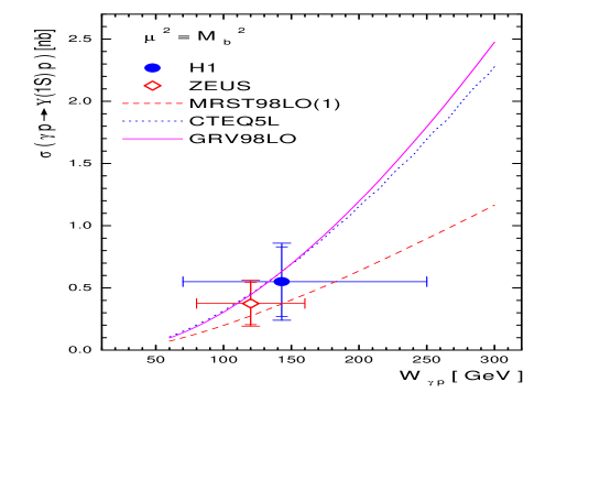
Figure 4: The cross section of elastic photoproduction of $\Upsilon(1S)$ versus $W_{\gamma p}$, the photon-proton center-of-mass energy. The data points are published HERA results[25]. The theoretical predictions of present work using various parameterizations of the gluon density in the proton at $m_{b}$ scale are also shown.

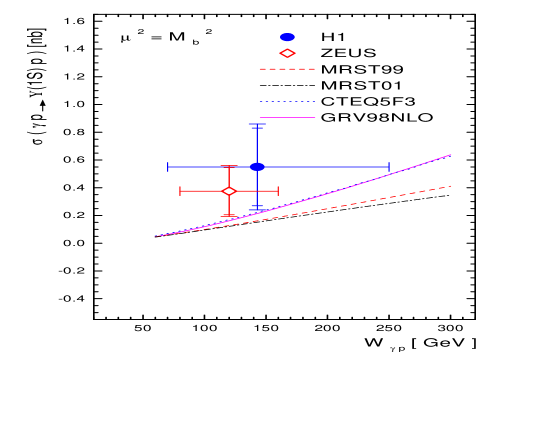
Figure 5: The cross section of elastic photoproduction of $\Upsilon(1S)$ versus $W_{\gamma p}$, the photon-proton center-of-mass energy. The data points are published HERA results[25]. The theoretical predictions of present work using various parameterizations of the gluon density in the proton at $m_{b}$ scale are also shown.

For $\Upsilon$ our predictions are obtained by taking $\mu=m_{b}=5$GeV. The discussed corrections should be small for the case with $\Upsilon$. We indeed find that our prediction with leading order gluon distributions is in agreement with experiment, although the experimental errors are large. Our numerical results are shown with experimental data[25] in Fig.4 with leading order gluon distributions, and in Fig.5 with the next-to-leading order gluon distributions. The contribution of the real part of the amplitude to the cross section is at $36\%$-, $43\%$- and $47\%$ level with the leading order gluon distribution of MRST98LO, CTEQ5L and GRV98LO, respectively. With the next-to-leading order gluon distribution of MRST01, MRST99, CTEQF3 and GRV98 it is at $20\%$-, $23\%$-, $29\%$- and $33\%$ level, respectively. For $\Upsilon$ productions another possible correction besides those discussed before is that at $\mu=m_{b}$ the finite skewness, which we have neglected to relate the S-matrix element to the gluon distribution, can lead a significant effect. Studies in [26, 27] show that this is the case. Instead using gluon distribution one may need to use the skewed gluon distribution to make numerical predictions. However, this distribution is not well known and numerical predictions cannot be made. It deserves a further study of corrections to our results both for $J/\psi$ and for $\Upsilon$.

5. Summary

In this work we have studied diffractive photoproduction of $J/\psi$, where we have taken the gluons exchanged between the initial hadron and the $c\bar{c}$ pair as soft gluons. We then have used an expansion in $m_{c}^{-1}$ to study the effect of the exchange of soft gluons. Our results have been derived with the assumption the exchange of two gluons in a special gauge. But, they can also be derived without the assumption in an arbitrary gauge. This can be done by formulating the problem as the splitting of the photon into a $c\bar{c}$ pair in a background field of gluons, which varies slowly in the space-time. Our results for the S-matrix element consist of a NRQCD matrix element representing the nonperturbative effect related to $J/\psi$ and a matrix element of two gluonic field strength operators which are separated in the moving direction of $J/\psi$ in the space-time. The matrix element of the field strength operators characterize the nonperturbative effect related to the initial hadron. In the limit of $s\rightarrow\infty$ the forward S-matrix element is related to the skewed gluon distribution. With a reasonable assumption the forward S-matrix element can also be related to the usual gluon distribution, this enables us to make numerical predictions and to compare with experiment.

Since we take the exchanged gluons as soft gluons, it is not very clear how to identify the renormalization scale $\mu$ to make numerical predictions. However, with the knowledge about the asymptotic behavior of the gluon distribution $g_{h}(x)$ with $x\rightarrow 0$ our results show that the total cross section increases with increasing energy. We first take $\mu$ as a soft scale and fit experimental results for $J/\psi$ with our results. The experimental data show clearly that the cross-section increases with the energy as $W^{\delta}$. With determined parameters we can predict the cross section for $\Upsilon$. However, the predicted cross sections are too small. Possible reasons are large corrections to the leading order results for $J/\psi$. We also take $\mu$ as a hard scale, i.e., as the mass of the heavy quark, with an existing gluon distribution we are able to give a rather good description of describe experimental data for $J/\psi$, although large corrections are neglected. These corrections for $\Upsilon$ are expected to be smaller those for $J/\psi$. We indeed find that our predictions with leading order gluon distributions for $\Upsilon$ production are in agreement with experiment, but there are only two data points with large errors. It deserves a further study of corrections to our results and of experiment.

Our approach is distinctly different than previous approaches. In previous approaches one start to use perturbative QCD to study diffractive production with a virtual photon in the initial state, where the virtuality $Q^{2}$ of the photon is large to ensure that perturbative QCD can be used for gluon exchange. Keeping leading order in $Q^{-2}$ and the finite mass of quarkonia one obtains results for the cross section. Then the cross section of diffractive production of a real photon is obtained by setting $Q^{2}=0$. Clearly, this setting can not be done properly, because higher orders in $Q^{-2}$ are neglected. In our approach we take the exchanged gluons as soft gluons and use an expansion in the inverse of the heavy quark mass to handle the exchange of soft gluons. Although the forward S-matrix element can be related to the gluon distribution as that in the previous approaches, but the relation is different, as discussed in detail in Sec. 3.

In our approach corrections can be systematically added. Among them relativistic correction can be most important for production of $J/\psi$, and a study of the relativistic correction is underway for getting accurate results of theory. With the accurate results of theory diffractive photoproduction may provide an interesting way to study the nonpertubative nature of nucleon and of nuclei.

Acknowledgments

The work of J. P. Ma is supported by National Nature Science Foundation of P. R. China and by the Hundred Young Scientist Program of Academia Sinica of P. R. China, the work of J. S. Xu is supported by the Postdoctoral Foundation of P. R. China and by the K. C. Wong Education Foundation, Hong Kong.

Appendix

In this appendix we study the integral which appears in Eq.(48). We define

$$I(\beta)=\int_{0}^{\infty}d\lambda\lambda^{-\beta}(\cos(\lambda)+i\sin(\lambda))=\int_{0}^{\infty}d\lambda\lambda^{-\beta}e^{i\lambda},$$ (76)

where $\beta$ is real. We make an exchange of variable $\lambda^{1-\beta}=z$, then the integral becomes

$$I(\beta=1-\alpha)=\frac{1}{\alpha}\int_{0}^{\infty}dz\exp(iz^{\frac{1}{\alpha}}).$$ (77)

Figure 6: The integration contour in complex $z-$plane.

We extend the integrand as a complex function and consider the contour integral where the contour in the complex $z$-plan is specified as in Fig. 6 with $\theta=\frac{1}{2}\alpha\pi$. Using the contour integral we have:

$$I(\beta=1-\alpha)=-\frac{1}{\alpha}\exp(i\frac{1}{2}\alpha\pi)\int_{0}^{\infty}dR\exp(-R^{\frac{1}{\alpha}}),$$ (78)

for $\alpha>0$ the integral is finite and it is real. With this result we obtain

$$\int_{0}^{\infty}d\lambda\lambda^{-\beta}\sin(\lambda)=\tan(\frac{1}{2}\alpha\pi)\int_{0}^{\infty}d\lambda\lambda^{-\beta}\cos(\lambda)$$ (79)

which is used in Eq.(48).

References

[1] S.J. Brodsky et al., Phys. Rev. D50 (1994) 3134
[2] M.G. Ryskin, Z. Phys. C57 (1993) 89
M.G. Ryskin et al., ibid., C76 (1997) 231
[3] J.C. Collins, L. Frankfurt and M. Strikman, Phys. Rev.
D56 (1997) 2982
J.C. Collins and A. Freund, Phys. Rev. D59 (1999) 074009
[5] N. Isgur and M.B. Wise, Phys. Lett. B232 (1989) 113, it ibid.
B237 (1990) 527
E. Eichten and B. Hill, Phys. Lett. B234 (1990) 511
B. Grinstein, Nucl. Phys. B339 (1990) 253
H. Georgi, Phys. Lett. B240 (1990) 447
[6]G.T. Bodwin, E. Braaten, and G.P. Lepage,
Phys. Rev. D51, 1125 (1995); Erratum:ibid., D55,
5853 (1997)
[7] J.P. Ma, Nucl. Phys. B602 (2001) 572
[8] J.P. Ma and Jia-Sheng Xu, Preprint AS-ITP-2001-016, hep-ph/0109055
[9] O. Nachtmann, Ann. Phys. Vol. 209 (1991) 436
[10] B. Blattel, G. Baym, L. Frankfurt and M. Strikman, Phys. Rev. lett.,
71 (1993) 896
L. Frankfurt, A. Radyushkin and M. Strikman, Phys. Rev. D55 (1997) 98
[11] L.L. Frankfurt, W. Koepf and M. Strikman, Phys. Rev. D57 (1998) 512
ibid., D54 (1996) 3194
[12] L. Frankfurt, M. McDermott and M. Strikman, JHEP 0103 (2001) 045
[13] J.C. Collins and D. Soper, Nucl. Phys. B194 (1982) 445
[14] X. Ji, J.Phys. G24 (1998) 1181
[15] A.D. Martin, M.G. Ryskin and Y. Teubner, Phys. Lett. B454 (1999) 339
[16] H1 Collaboration, C. Adloff et al., Phys. Lett. B483 (2000) 23;
S. Aid et al., Nucl. Phys. B472 (1996) 3,
ZEUS Collaboration, J. Breitweg et al., Z. Phys. C75 (1997) 215;
M. Derrick et al., Phys. Lett. B350 (1995) 120
[17] P.B. McKenzie and G.P. Lepage, Phys. Rev. Lett. 47 (1981) 1244
W. Celmaster, Phys. Rev. D19 (1979) 1517
[18] M. Beneke, A. Signer and V.A. Smirnov, Phys.Rev.Lett. 80 (1998) 2535
[19] J.P. Ma, Phys.Rev. D62 (2000) 054012
[20] M. Glück, E. Reya and A. Vogt, Eur. Phys. J. C5 (1998) 461
[21] H. L. Lai et al., Eur. Phys. J. C12 (2000) 375
[22] A. D. Martin, R. G. Roberts, W. J. Stirling and R. S. Thorne,
Eur. Phys. J. C14 (2001) 133
[23] A. D. Martin, R. G. Roberts, W. J. Stirling and R. S. Thorne,
Phys. Lett. B443 (1998) 301
[24] A. D. Martin, R. G. Roberts, W. J. Stirling and R. S. Thorne, hep-ph/0110215
[25]ZEUS Collaboration, J. Breitweg et al., Phys. Lett. B437 (1998) 432;
H1 Collaboration, C. Adloff at al., Phys. Lett. B483 (2000) 23
[26] A.D. Martin and M.G. Ryskin, Phys. Rev. D57 (1998) 6692
[27] L.L. Frankfurt, M.F. McDermott and M. Strikman, JHEP 9902 (1999) 002