Cumulative particle production and percolation of strings

Abstract. Calculations of the production rate of particles with $x>1$ in nuclear collisions due to the interaction of colour strings are presented. Momentum and colour sum rules are used to determine the fragmentation functions of fused strings. Mechanisms of the string interaction are considered with total and partial overlapping in the transverse plane. The results reveal strong dependence of the chosen mechanism. In the percolation scenario with partial overlapping the $x$-dependence of the production rates agrees well with the existing data. The magnitude of the rates for $\pi^{+}$ production is in agreement with experiment. However the rates for the protons are substantially below the data.

1 Introduction

Production of particles in nuclear collisions in the kinematical region prohibited in the free nucleon kinematics (”cumulative particles”) has long aroused interest both from the theoretical and pragmatic point of views. On the pragmatic side, this phenomenon, in principle, allows to raise the effective collision energy far beyond the nominal accelerator one. This may turn out to be very important in the near future, when all possibilities to construct still more poweful accelerator facilities become exhausted. Of course one should have in mind that the production rate falls very rapidly above the cumulative threshold, so that to use the cumulative effect for practical purposes high enough luminosities are necessary. On the theoretical side, the cumulative effect explores the hadronic matter at high densities, when two or more nucleons overlap in the nucleus. Such dense clusters may be thought to be in a state which closely resembles a cold quark-gluon plasma. Thus cumulative phenomena could serve as an alternative way to produce this new state of matter.

There has never been a shortage of models to describe the cumulative phenomena, from the multiple nucleon scattering mechanism to repeated hard interquark interactions [1]. However it should be acknowledged from the start that the cumulative particle production is at least in part a soft phenomenon. So it is natural to study it within the models which explain successfully soft hadronic and nuclear interactions in the non-cumulative region. Then one could have a universal description of particle production in all kinematical regions. The non-cumulative particle production is best described by the colour string models, in which it is assumed that during the collisions colour strings are stretched between the partons of colliding hadrons (or nuclei), which then decay into more strings and finally into observed produced hadrons

It is clear that if the strings are formed independently for different partons, all the cumulative effect can be generated exclusively by the partonic movement. This can lead to cumulative particles due to the Fermi-motion of the nucleons in the participant nuclei. However in all realistic nuclear models the Fermi-motion generates cumulative particles only in the region immediately above the cumulative threshold. Beyond the threshold the effect dies so quickly that there is absolutely no hope to explain by the Fermi-motion the experimentally known production rates at $x\sim 2\div 3$ . Thus in the string models the cumulative effect is related to the interaction between strings, in particular, to their fusion, which creates strings of higher energy and thus of a longer length in rapidity. A model of string fusion and their percolation was proposed by the authors some time ago [2]. It proved to be rather successful in explaining a series of phenomena related to collective effects among the produced strings, such as damping of the total multiplicity and strange baryon enhancement. Calculations of the production rates in the cumulative region made by the Monte-Carlo algorithm allowing for fusion of only two strings gave encouraging results [3]. They agree quite well with the existing data for hA collisions at $E_{cm}=27.5$ GeV [4,5 ]. However to pass to higher energies and heavy-ion collisons one has to consider a possibility of interaction of many strings. In this note we study such an interaction using a simplified model in which both colour and energy-momentum conservation are imposed on the average.

From the start it is not at all obvious that the colour string approach may give reasonable results in the deep fragmentation region, near the kinematical threshold. The string picture has been introduced mainly to describe particle production in the central region, where its results agree with the data very well. It turned out however that it gives a quite reasonable description of the pion production also in the fragmentation region. The baryon spectra in the nucleus fragmentation region, on the contrary, are very poorly described, which circumstance is standardly ascribed to the interaction between nucleons as a whole [6]. So, moving still further into a cumulative region, we may only expect a reasonable description for the production of pions, and not of baryons. As we shall see from our results, this is indeed so. We get a very reasonable description of the pion production rates for $1<x<2$ at 27.5 GeV [5] but we are not able to describe the proton rates, which are experimentally two orders of magnitude greater than our predictions. Obviously the bulk of cumulative protons come from a different mechanism, which does not involve colour string formation but rather interactions of nucleons as a whole. Such a mechanism was included in the Monte-Carlo code of [3], which is the reason why it gave results for nucleon production in agreement with the experimental data.

2 The model

The fully extended string model assumes that each of the colliding hadrons consists of partons (valence and sea quarks), distributed both in rapidity and transverse space with a certain probability, deduced from the experimentally known transverse structure and certain theoretical information as to the behaviour of the $x$ distributions at $x=0$ and $x=1$. These distributions are taken to be the ones for the endpoints of the generated strings. As a result, the strings aquire a certain length in rapidity. We shall choose the c.m. system for the colliding hadrons with the nucleus (projectile) moving in the forward direction. The cumulative particles thus will be observed in the forward hemisphere.

Let a parton from the projectile carry a part $x_{1+}$ of the ”+” component of its momentum $p_{1}$ and a partner parton from the target carry a part $x_{2-}$ of the ”-” component of its momentum $p_{2}$. The total energy squared for the colliding pair of nucleons is

$$S=2p_{1+}p_{2-}=m^{2}e^{Y}$$ (1)

where $m$ is the nucleon mass and $Y$ is the total rapidity available. The c.m. energy squared accumulated in the string is then

$$s=x_{1+}x_{2-}S$$ (2)

Note that the concept of a string has only sense in the case when $s$ is not too small, say more than $m^{2}$. So both $x_{1+}$ and $x_{2-}$ cannot be too small.

$$x_{1+},x_{2-}>x_{min}=m/\sqrt{S}=e^{-Y/2}$$ (3)

Correspondingly we relate the scaling variables for the string endpoints to their rapidities by

$$y_{1}=Y/2+\ln x_{1+},\ \ y_{2}=-Y/2-\ln x_{2-}$$ (4)

Due to (3) $y_{1}\geq 0$ and $y_{2}\leq 0$. The ”length” of the string is just the difference $y_{1}-y_{2}$.

Standardly it is assumed that the spectrum of observed particles generated by the string is nearly a constant along its length and zero outside. Due to the partonic distribution in $x$ the strings have different lengths and moreover can take different position respective to the center $y=0$. The sea distribution in a hadron is much softer than the valence one. In fact the sea distribution behaves as $1/x$ near $x=0$, so that the average value of $x$ for sea partons is of the order $1/Y$ (see Eq. (3)). As a result, strings attached to sea partons in the projectile nucleus carry very small parts of longitudinal momentum in the forward direction, which moreover fall with energy, so that they seem to be useless for building up the cumulative particles. This allows us to retain only strings attached to valence partons, quarks and diquarks, in the projectile and neglect all strings attached to sea quarks altogether. Note that the number of the former is exactly equal to $2A$ and does not change with energy. So for a given nucleus we shall have a fixed number of strings, independent of the energy.

The upper end rapidities of the strings attached to diquarks are usually thought to be larger than of those attached to the quarks, since the average value of $x$ for the diquark is substantially larger that for the quark. Theoretical considerations lead to the conclusion that as $x\to 1$ the distributions for the quark and diquark in the nucleon behave as $(1-x)^{3/2}$ and $(1-x)^{-1/2}$ respectively, modulo logarithms [6]. Neglecting the logarithms and taking also in account the behaviour at $x\to 0$ we assume that these distributions are

$$q(x)=\frac{8}{3\pi}x^{-1/2}(1-x)^{3/2}$$ (5)

for the quark and

$$qq(x)=q(1-x)=\frac{8}{3\pi}x^{3/2}(1-x)^{-1/2}$$ (6)

The quark and diquark strings will be attached to all sorts of partons in the target nucleon: valence quark and diquark and sea quarks. Their position in rapidity in the backward hemisphere will be very different. However we are not interested in the spectrum in the backward hemisphere. So, for our purpose, limiting ourselves with the forward hemisphere, we may take lower ends of the strings all equal to $x_{min}<<1$. As a result, in our model at the start we have $N$ initially created strings, half of them attached to quarks and half to diquarks, their lower ends in rapidity all equal to

$$y_{2}=Y/2+\ln x_{min}$$

and their upper ends distributed in accordance with (5) and (6). As soon as they overlap in the transverse space they fuse into new strings with more color and more energy. This process will be studied in the next section.

3 String fusion and conservation laws

3.1 Complete fusion

Let $n$ strings overlap completely in the transverse area and form a new string of higher colour. The process of fusion obeys two conservation laws: those of colour and momentum. As a result of the conservation of colour, the colour of the fused string is $\sqrt{n}$ higher than that of the ordinary string [7,8]. From the 4 momentum conservation laws we shall be interested mostly in the conservation of the ”+” component, which leads to the conservation of $x$. The fused string will have the upper endpoint with $x_{n}=\sum_{i=1}^{n}x^{(i)}$, where $x^{(i)}$ are upper ends of fusing strings(we omit the subscripts ”1+”, since we shall be interested only in these variables in the future).

These properties of the fused string transform into certain sum rules which restrict a possible form of the spectrum of produced hadrons. Let us first assume that only one sort of particles is produced and let the mutiplicity density (”fragmentation function” in the terminology of [6]) of the fused string be

$$\tau_{n}=\frac{d\mu_{n}}{dy}$$

where $\mu$ is the multiplicity. As mentioned, the total number of particles produced in the forward hemisphere by the fused string should be $\sqrt{n}$ greater than by the ordinary string. This leads to the multiplicity sum rule:

$$\int_{x_{min}}^{x_{n}}\frac{dx}{x}\tau_{n}(x)=\frac{1}{2}\mu_{0}\sqrt{n}$$ (7)

where we denote $\mu_{0}$ the total multiplicity from a simple string. The produced particles have to carry all the longitudinal momentum in the forward direction. This results in the sum rule for $x$:

$$\int_{x_{min}}^{x_{n}}dx\tau_{n}(x)=x_{n}$$ (8)

In these sum rules $x_{min}$ is given by (3) and is small. Passing to the scaled variable $z=x/x_{n}$ we rewrite the two sum rules as

$$\int_{z_{n}}^{1}\frac{dz}{z}\tau_{n}(z)=\frac{1}{2}\mu_{0}\sqrt{n}$$ (9)

and

$$\int_{z_{n}}^{1}dz\tau_{n}(z)=1$$ (10)

where

$$z_{n}=x_{min}/x_{n}$$ (11)

These sum rules put severe restrictions on the form of the distribution $\tau_{n}$, which obviously cannot be independent of $n$. Comparing (7) and (8) we see that the spectrum of the fused string has to vanish at its upper threshold faster than for the simple string. In the scaled variable $z$ it is shifted to smaller values (and thus to the central region). This must have a negative effect on the formation of cumulative particles produced at the extreme values of $x$.

To proceed, we choose a simplest form for the distribution $\tau_{n}$:

$$\tau_{n}(z)=a_{n}(1-z)^{\alpha_{n}-1}$$ (12)

The $x$ sum rule relates $a_{n}$ and $\alpha_{n}$:

$$a_{n}=\alpha_{n}(1-z_{n})^{-\alpha_{n}}\simeq\alpha_{n}$$ (13)

The multiplicity sum rule finally determines $\alpha_{n}$:

$$\alpha_{n}(1-z_{n})^{-\alpha_{n}}\int_{z_{n}}^{1}\frac{dz}{z}(1-z)^{\alpha_{n}-1}=\frac{1}{2}\mu_{0}\sqrt{n}$$ (14)

These equation can be easlily solved when $z_{n}\to 0$ We present the integral in (14) as

$$\int_{z_{n}}^{1}\frac{dz}{z}[(1-z)^{\alpha_{n}-1}-1]+\ln\frac{1}{z_{n}}$$ (15)

The integral term is finite at $z_{n}=0$ so that we can write it as a difference of integrals in the intervals $[0,1]$ and $[0,z_{n}]$. The first can be found exactly

$$I_{1}=\int_{0}^{1}\frac{dz}{z}[(1-z)^{\alpha_{n}-1}-1]=\lim_{\epsilon\to 0}\int_{0}^{1}dzz^{-1+\epsilon}[(1-z)^{\alpha_{n}-1}-1]=$$

$$\lim_{\epsilon\to 0}\Big{[}{\rm B}(\alpha_{n},\epsilon)-\frac{1}{\epsilon}\Big{]}=\psi(1)-\psi(\alpha_{n})$$ (16)

The second term has an order $-(\alpha_{n}-1)z_{n}$ and is small unless $\alpha_{n}$ grows faster than $n$, which is not the case as we shall presently see. In fact we shall find that $\alpha_{n}$ grows roughly as $\sqrt{n}$, which allows to neglect the second factor in (14) and rewrite it in its final form

$$\alpha_{n}\Big{[}\ln\frac{1}{z_{n}}+\psi(1)-\psi(\alpha_{n})\Big{]}=\frac{1}{2}\mu_{0}\sqrt{n}$$ (17)

Obviously $\alpha_{n}$ grows as $\sqrt{n}$, modulo logarthmic dependence, as mentioned. To finally fix the distributions we have to choose the value of $\alpha$ for the simple string. We take the simplest choice $\alpha_{1}=1$ for an average string with $x=x_{0}=1/2$, which corresponds to a completely flat spectrum and agrees with the results of [6]. This fixes the multiplicity density for the average string

$$\tau_{1}(y)=1$$ (18)

which favorably compares to the value 1.1 extracted from the experimental data [8].

With (18) we find from (17)

$$\frac{1}{2}\mu_{0}=\ln\frac{1}{z_{0}},\ \ z_{0}=\frac{x_{min}}{x_{0}}$$ (19)

and the equation (17) can be rewritten as

$$\alpha_{n}\Big{[}\ln\frac{n}{z_{0}}+\psi(1)-\psi(\alpha_{n})\Big{]}=\sqrt{n}\ln\frac{1}{z_{0}}$$ (20)

One concludes that at $S\to\infty$ the solution is $\alpha_{n}=\sqrt{n}$. However this is modified by logarithmic terms when $n$ is high enough: $n\sim\sqrt{S}/m$. At finite $S$ Eq. (20) can be solved numerically for $\alpha_{n}$

In any case, we find that with the growing $n$ the spectrum of produced particles goes to zero at $z\to 1$ more and more rapidly. So although strings with large $n$ produce particles with large values of $x\leq x_{n}$, the production rate is increasingly small.

3.2 Partial fusion

Now we pass to a more difficult case when two or more strings only overlap partially. This case corresponds to weaker interaction between strings, which retain their form in the transverse space. This case lies at the basis of the percolation phenomenon. To start, let us note that for two or several completely independent strings the conservation laws and the following sum rules are automatically satisfied if they are satisfied for each string individually. As a consequence the case of partially fusing strings has to be treated differently depending on whether we consider a formed cluster as a single string or as a set of many strings formed by the various areas where a fixed number of particular strings overlap. In the first case we have to impose a single pair of conservation laws for the whole cluster. In the second case we find many pairs of conservation laws for strings formed by different overlaps.

An approach which admits the most direct physical interpretation is to consider a cluster of $n_{c}$ strings as a set of many independent “ministrings” formed by different overlaps. This case corresponds to the minimal interaction between strings, which actually only superimpose in the transverse space without changing any of their properties. In this case the conservation laws and sum rules have to be imposed for each particular overlap. If the area of a given overlap of $n$ strings is $S_{n}^{(i)}$, where $i$ enumerates different overlaps of $n$ strings, then the colour of the corresponding ministring is [8]:

$$Q_{n}^{(i)}=\sqrt{n}\frac{S_{n}^{(i)}}{C_{1}}Q_{0}$$ (21)

where $Q_{0}$ is the colour if the simple string and $C_{1}$ is its area.. As a result, the total multiplicity will be changed correspondingly. Passing to the momentum, we have to assume some manner in which the total $x=x_{c}$ of the cluster is distributed among various ministrings formed by overlaps. A natural way (similar to the one used for the distributiuon of color) is to assume that the part of the longitudinal momentum shared by a string in a particular overlap is proportional to the area of the latter. Then the total $x$ of the overlap is:

$$x_{n}^{(i)}=x_{c}\frac{nS_{n}^{(i)}}{n_{c}C_{1}}$$ (22)

where $n_{c}$ is the number of strings forming the cluster. Indeed, since

$$\sum_{i,n}nS_{n}^{(i)}=n_{c}C_{1}$$ (23)

we have for each cluster

$$\sum_{i,n}x_{n}^{(i)}=x_{c}$$ (24)

as it should be. Introducing for each individual overlap its scaled variable $z=x/x_{n}^{(i)}$ we shall write the momentum sum rule in the same form (10) as before. The multiplicity sum rule will now read

$$\int_{z_{n}^{(i)}}^{1}\frac{dz}{z}\tau_{n}(z)=\frac{1}{2}\mu_{0}\sqrt{n}\frac{S_{n}^{(i)}}{C_{1}}$$ (25)

where

$$z_{n}^{(i)}=x_{min}/x_{n}^{(i)}.$$

With the choice (12) the final equation for $\alpha_{n}$ will take the form

$$\alpha_{n}\Big{[}\ln\frac{1}{z_{n}^{(i)}}+\psi(1)-\psi(\alpha_{n})\Big{]}=\ln\frac{1}{z_{0}}\sqrt{n}\frac{S_{n}^{(i)}}{C_{1}}$$ (26)

Obviously calculations cannot be done analytically now but require numerical simulation. They result very time consuming, since one has to identify each particular overlap in each cluster.

A simpler alternative is to treat the whole cluster as a single string of a complicated form and area $C_{n}$, with properties intermediate between $n$ separate strings and completely fused ones. This implies a considerable amount of interaction between strings, which redistributes the colour and momentum homogeneously over the cluster area. Let the cluster of $n$ strings have the total $x$ equal to $x_{c}$. However the maximal momentum $x_{n}$ of the emitted particle cannot be equal to $x_{c}$, since for $n$ separate strings just touching each other it is only $x_{1}$. So it should be intermediate between $x_{1}$ and $x_{c}$, depending on the fusion intensity. A natural choice seems to be

$$x_{n}=x_{c}\frac{C_{1}}{C_{n}}$$ (27)

In fact for $n$ independent strings $C_{n}=nC_{1}$ and $x_{n}=x_{c}/n$, which is just an average of the maximal momenta of fusing strings. For $n$ completely fused strings $C_{n}=C_{1}$ and $x_{n}=x_{c}$ as it should be. The momentum sum rule is then

$$\int_{x_{min}}^{x_{n}}dx\tau_{n}(x)=x_{c}$$ (28)

Taking

$$z=\frac{x}{x_{n}},\ \ \tau=\frac{x_{c}}{x_{n}}\tilde{\tau}$$ (29)

we obtain an equation for $\tilde{\tau}$ of the same form as (25) with $z_{n}=x_{min}/x_{n}$ The total multiplicity will be also intermediate between the multiplicity of $n$ independent strings and of the completely fused string. A reasonable choice similar to (27) is [9]

$$\mu_{c}=\mu_{0}\sqrt{n\frac{C_{n}}{C_{1}}}$$ (30)

This will lead to the corresponding change in the multiplicity sum rule, which in terms of $z$ and $\tilde{\tau}$ becomes

$$\int_{z_{n}}^{1}\frac{dz}{z}\tilde{\tau}_{n}(z)=\frac{1}{2}\mu_{0}\sqrt{n\frac{C_{1}}{C_{n}}}$$ (31)

For $n$ independent strings (31) goes into (7) with $n=1$. For complete overlapping, when $C_{n}=C_{1}$, (30) reproduces (7). With the choice (12) for the distribution in rapidity we now get an equation for $\alpha_{C}$

$$\alpha_{C}\Big{[}\ln\frac{1}{z_{n}}+\psi(1)-\psi(\alpha_{C})\Big{]}=\ln\frac{1}{z_{0}}\sqrt{n\frac{C_{1}}{C_{n}}}$$ (32)

This equation has to be solved separately for each cluster, so that the form of the distribution of particles produced by a cluster of $n$ strings will depend on its geometry (in fact only on its total area). The numerical calculations look easier now, since one has to identify individual clusters only.

3.3 Various types of hadrons

In reality various types of hadrons are produced. In the cumulative region the relevant particles are nucleons and pions, the production rates of the rest being much smaller. The multiplicity densities for each sort of hadrons will obviously depend on the flavour contents of the fused strings, that is, of the number of quark and diquark strings in it.

Consider the case of complete overlapping of $n$ strings. Let the string be composed of $k$ quarks and $n-k$ diquarks. We shall then have distributions $\tau_{nk}^{(h)}$ for the produced hadrons $h$. Obviously the multplicity and momentum sum rules are now insufficient to determine each of the distribution $\tau_{nk}^{(h)}$ separately. A possibility to overcome this difficulty may consist in using the Regge phenomenology or quark power counting rules to determine the behaviour of the distribution near its kinematical threshold $x\rightarrow x_{n}$. However for multiquark configurations this seems too complicated and insecure, since this behaviour is then governed by Regge cuts rather than poles. Therefore we shall adopt a simpler approach. In our picture the observed hadron is produced when the parton (quark or diquark) emerging from string decay neutralizes its colour by picking up an appropriate parton from the vacuum. In this way a quark may go into a pion if it picks up an antiquark or into a nucleon if it picks up two quarks. The quark counting rules tell us that the behaviour at the threshold in the second case will have two extra powers of $(x-x_{n})$. Likewise a diquark may go either into a nucleon picking up a third quark or into two pions picking up two antiquarks, with a probability smaller by a factor $(x-x_{n})^{2}$ at the threshold. Since it is the threshold behaviour which is responsible for the cumulative particles, we shall assume, as a first approximation, that the quarks go exclusively into pions and diquarks go exclusively into nucleons. As a result, the ratio of produced pions to nucleons will be equal to that of quarks to diquarks, that is, $k/(n-k)$.

This means that we may proceed as before assuming one sort of hadrons and in the end just multiply the obtained distributions $\tau_{nk}$ by the appropriate factors

$$\tau_{nk}^{(h)}(x)=\xi_{nk}^{(h)}\tau_{mk}(x),$$ (33)

where for the pions and nucleons

$$\xi_{nk}^{(\pi)}=\frac{k}{n},\ \ \xi_{nk}^{(N)}=\frac{n-k}{n}$$ (34)

Obviously this implies that we have to track the flavour contents of the fused strings in the Monte-Carlo simulations.

4 Numerical results

We shall study different scenarios for the interaction between colour strings. We start with the scenario of string fusion, when as soon as the strings touch each other they fuse into a new one with a higher colour and of the same form and transverse area as the initial ones. This corresponds to the maximal interaction between strings, which change not only their colour and momentum but also its geometrical form. This scenario was proposed and realized in a fully developed Monte-Carlo algorithm in [2]. Its application to particle production has given very satisfactory results for energies ranging from SPS to RHIC [10].

In this case we do not have to bother about partial overlapping, so that Eq. (20) can be used directly to determine the multiplicity of a string with an arbitrary high colour. The distribution of the strings in colour can be deduced analitically for high enough string densities in this scenario [11]. It is governed by a dimensionless parameter

$$\eta=\frac{NC_{1}}{C}$$ (35)

where $C$ is the total transverse area of the interaction and $N$ the total number of strings. For a given $\eta$ and large $N$ one finds that the strings are distributed in colour according to the Poisson law:

$$\langle\nu_{n}\rangle=Ne^{-\eta}\eta^{n-1}/n!$$ (36)

So with string fusion we find the total multiplicity as

$$\frac{d\mu}{dy}=N\sum_{n}\frac{1}{n!}e^{-\eta}\eta^{n-1}\alpha_{n}\left(1-\frac{x}{x_{n}}\right)^{\alpha_{n}-1},$$ (37)

where the sum goes over all colors $n$ such that $x<x_{n}$. Parameters $\alpha_{n}$ are to be calculated from Eq. (20) and the string momentum $x_{n}$ and its flavour composition (number of quarks and diquarks) has to be found by Monte-Carlo simulations using the distributions (5) and (6).

The multiplicity results very weakly dependent on the energy through the value of $x_{min}$ (eq. (3)), this dependence practically absent for energies above 200 GeV. Our results for $d\mu/dy$ per string at the LHC energy 6 TeV (Y=17.5) for different values of $\eta$ are presented in Fig. 1 and 2 for pions and nucleons respectively.

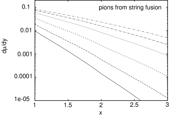
Figure 1: Multiplicity density $d\mu/dy$ per string for pions in the fusion scenario for $Y=17.5$. The curves from bottom upwards correspond to $\eta=0.25$, 0.5, 1, 2, 3 and 4.

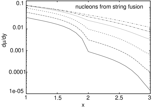
Figure 2: Same as Fig. 1 for nucleons.

In an alternative scenario, which lies at the basis of the percolation phenomenon (”percolation scenario”) strings are allowed to overlap partially and form clusters of different forms and number of simple strings. The total multiplicity will then depend on the chosen model of the distribution of colour and momentum within a given cluster, as explained in the previous section.

If a cluster is assumed to be split in various ministrings formed by different separated overlaps, the total multiplicity will be a sum of contributions from all ministrings

$$\frac{d\mu}{dy}(x)=\sum_{n,i}\tau_{n,i}\left(\frac{x}{x_{n}^{(i)}}\right)$$ (38)

where for $z<1$ $\tau_{n,i}(z)$ is given by (12) with parameters $\alpha_{n,i}$ determined from Eq. (26) and for $z>1$ $\tau_{n,i}(z)=0$. If a cluster acts as a single string with an averaged distribution $\tau_{C}(z)$ described in a previous section, then one has the same expression (38), where the sum is now extended over all clusters. The parameters $\alpha_{C}$ are now to be determined from Eq. (32). In both cases analytical calculations are not possible and one has to recur to Monte Carlo simulations. They simulate the geometrical distribution of strings in the interaction area and their $x$ and flavour contents. Afterwards one has to identify all overlaps of a given number of strings or clusters of strings and their areas. The results (per string) for the two possibilities are presented in Figs. 3,4 and 5,6 respectively.

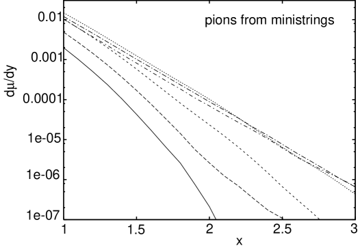
Figure 3: Multiplicity density $d\mu/dy$ per string for pions in the percolation scenario with ministrings (overlaps) as emitters at $Y=17.5$. At $x=2$ the curves from bottom upwards correspond to $\eta=0.25$, 0.5, 1, 4, 3 and 2.

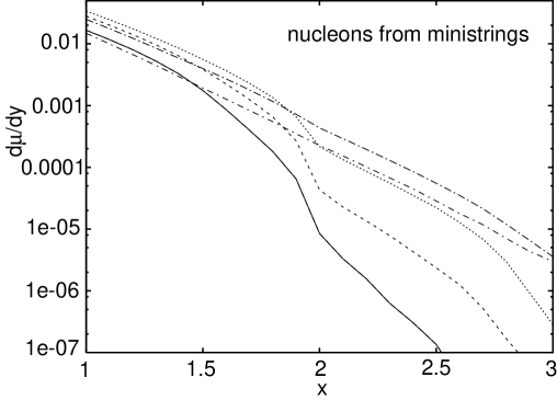
Figure 4: Same as Fig. 3 for nucleons. At $x=2.5$ the curves from bottom upwards correspond to $\eta=0.25$, 0.5, 4, 1, 3 and 2.

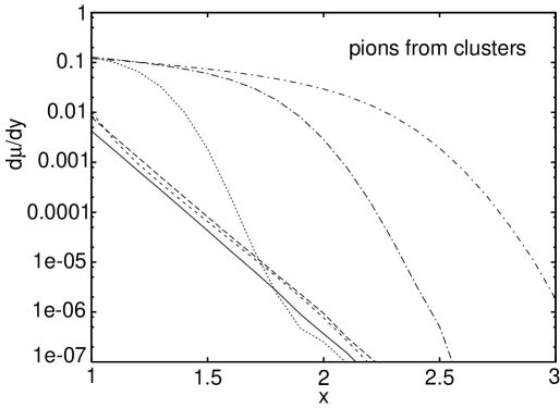
Figure 5: Multiplicity density $d\mu/dy$ per string for pions in the percolation scenario with clusters as emitters at $Y=17.5$. At $x=2$ the curves from bottom upwards correspond to $\eta=2$, 0.25, 1, 0.5, 3 and 4.

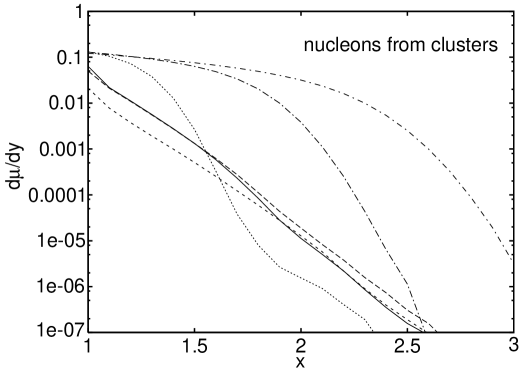
Figure 6: Same as Fig.5 for nucleons. At $x=2$ the curves from bottom upwards correspond to $\eta=2$, 0.25, 1, 0.5, 3 and 4.

One observes that probability of cumulative production strongly depends on a chosen scenario. The fusion scenario leads to higher cumulative particle production rates, which also fall with $x$ much slowlier than in the percolation scenario. The $x$-dependence of the rates for pion production is rather well described by the standard parametrization

$$\frac{d\mu}{dy}=Ce^{-\alpha x}$$ (39)

where the slope $\alpha$ steadily falls with $\eta$ from $\alpha\simeq 4$ at $\eta=0.25$ down to $\alpha\simeq 1.5$ at $\eta=4$. At fixed $x$ the rates steadily grow with $\eta$. For the nucleon production and low values of $\eta\leq 1$ the parametrization (39) holds only for the regions $1<x<1.7$ and $2<x<2.5$ where $\alpha\sim 2$. In between and at $x>2.5$ the slopes rise up to $4\div 6$ indicating an abrupt change of $x$-behaviour at $x\simeq 2$ which gradually disappears with the growth of $\eta$. At $\eta\geq 2$ the $x$-dependence is roughly described by (39) with the same slope $\sim 1.5$ as for pions.

In the percolation scenario at relatively small values of $\eta<1$ the results are qualitatively independent of the choice of emitters. With both clusters and ministrings one finds the rates which fall with $x$ much faster than in string fusion. Again for pions the parametrization (39) holds, with $\alpha$ slowly falling with $\eta$ from $\sim 9$ at $\eta=0.25$ to $\sim 6.5$ at $\eta=1.$ for ministrings as emitters and from $\sim 9.5$ at $\eta=0.25$ to $\sim 8.5$ at $\eta=1$ for clusters. For nucleon production from ministrings a change of behaviour in the vicinity of $x=2$ is again observed. With clusters this change is hardly perceptible. Outside this region the slopes are somewhat smaller than for pions: $4\div 7$ for ministrings and $7\div 9$ for clusters.

At higher values of $\eta$, beyond the percolation threshold $\eta_{c}\sim 1.1\div 1.3$, the behaviour of the production rate begins to depend crucially on the choice of emitters. With clusters as emitters a radical change is observed and the production rate becomes close to the fusion scenario up to a certain value of $x$ when the rate abruptly goes to zero. The critical value of $x$ grows with $\eta$ and, as seen from Fig.3, lies around 1.5 at $\eta=2$ and at around 2.5 at $\eta=4$. On the other hand, the ministrings scenario does not show such an abrupt change of behaviour, the rates well described by (39) with a slope $4\sim 5$ both for pions and nucleons.

To pass to physical inclusive cross-sections one has to know the number of strings $N$ in a particular reaction. This number is obtained by multiplying their number in the nucleon (two) by the number of collisions $\nu$.

In hA collisions in the nuclear fragmentation region one has

$$\nu=\frac{A\sigma_{pp}}{\sigma_{pA}}$$ (40)

The interaction area is of the order $\sigma_{pp}$, so that (35) gives

$$\eta=2\frac{AC_{1}}{\sigma_{pA}}$$ (41)

According to our previous results [2,3,8] $C_{1}=1.26$ mb. To find the inclusive cross-section one has to multiply $d\mu/dy$ per string by $N$ and $\sigma_{pA}$ and divide by the number of isospin components, which gives the inclusive cross-section per nucleon for positive pions and protons

$$\frac{1}{A}\frac{d\sigma_{pA}^{(\pi^{+})}}{dy}=\frac{2}{3}\sigma_{pp}\frac{d\mu^{(\pi)}}{dy},\ \ \frac{1}{A}\frac{d\sigma_{pA}^{(p)}}{dy}=\sigma_{pp}\frac{d\mu^{(N)}}{dy}$$ (42)

In AB interactions the number of collisions depends on the centrality. In minimum bias collisions, similar to (40),

$$\nu=\frac{AB\sigma_{pp}}{\sigma_{AB}}$$ (43)

The interaction area is the average overlap area. For $B<<A$ it is roughly equal to $\sigma_{pB}$. For $A=B$ it is approximately equal to $0.78R_{A}^{2}$. The inclusive cross-section per nucleon will be given by the same Eq. (42). the only difference being that the value of $\eta$ should be calculated with (43) and so substancially higher than in $hA$ collisons. One can also easily deduce corresponding formulas for the cross-sections in collisions with a given centrality, that is, at a given impact parameter $b$ (see [11]).

Passing to the comparison of our predictions with the experimental data we have first to stress that all the existing data refer to the hadron nucleus collisions at very moderate c.m. energies of 27.5 GeV and below. The strings which are created at these energies have mostly rather small length in rapidity, so that effects of the energy division between strings, neglected in our approach, become important. This implies that our picture can describe these experiments only rather crudely.

Still, forgetting for the moment the absolute magnitudes of the cross-sections, we conclude from Figs. 1-6 that the $x$-dependence is correctly reproduced in the two percolation scenarios, which at small $\eta$ corresponding to these energies give the inclusive cross-section of the form (39) with the slope $\alpha\sim 6\div 7$ in complete agreement with the experimental values. It is remarkable that this value of the slope is obtained practically with no parameters, on a pure geometrical basis. The string fusion scenario, in contrast, leads to much smaller values of $\alpha$ which definitely contradict the experimental data. So our first conclusion is that it looks as if the experimental cumulative cross-section favour the percolation scenarios.

Passing to the absolute values, we note that in [4,5] the double differential cross-sections in momentum and angle are given. To convert them into $d\sigma_{pA}/dy$ we fitted the data with

$$\frac{1}{A}\frac{d\sigma_{A}(x,k_{T}^{2})}{dyd^{2}k}=Ce^{-\alpha_{ex}x-\beta k_{T}^{2}}$$ (44)

For positive pions produced on $Ta$ (A=181) at $\sqrt{s}=27.5$ and $x>1$ we get

$$\alpha_{ex}=7.15,\ \beta=1.72\ \ {\rm and}\ \ C=124/{\rm mb/(GeV/c)}^{2}$$

The resulting ”experimental” $d\sigma_{A}/Ady$ is a pure exponential in $x$ with slope $\alpha_{ex}$ and is shown as a straight line in Fig. 7. In the same figure we show our predictions for this case ($\eta=0.343$) in the percolation scenarios choosing ministrings or clusters as emitters. One observes that the agreement is quite reasonable, especially in view of the mentioned difficulties in applying our picture.

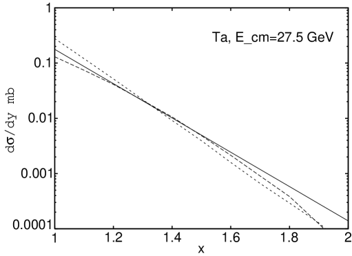
Figure 7: Comparison of the inclusive cross-sections for the production of cumulative $\pi^{+}$ on Ta at 27.5 GeV extracted from the experimental data [5] (straight line) and predictions from the percolation scenario with ministrings (lower curve at $x=1$) and clusters (upper curve at $x=1$) as emitters.

On the other hand, the cross-sections for the protons, result two order of magnitudes smaller than the experimental ones, which can be described by the same expression (49) with $\alpha=5.7$, $\beta=2.4$ and $C=28400$ in the same units. So our picture definitely does not work for the protons, at least at the energies corresponding to the experiment [4].

Guided by these results, we can make predictions for the cumulative $\pi^{+}$ production at energies corresponding to RHIC and LHC. Taking the inelastic cross-section $\sigma_{pp}$ equal to 39 and 77 mb at RHIC and LHC energies respectively, we find for Pb-Pb minimum bias collisons the corresponding values of $\eta$ equal to 2.0 and 4.0. So, using Eq. (42), we can read our predictions for the inclusive $\pi^{+}$ cross-section per nucleon (in mb)) directly from Figs. 3 and 5 multiplying $d\mu/dy$ at $\eta=2$ by 33 for RHIC and at $\eta=4$ by 43 for LHC.

One sees, that up to certain maximal $x$ ($\sim$ 1.6 at RHIC energy) the cross-sections with clusters as emitters are substantially higher than with ministrings. The difference reaches two orders of magnitude at $1.5<x<2.5$ for LHC energy. Beyond this maximal $x$ the cross-section with clusters abruptly goes to zero. Thus the study of cumulative pion production at higher energies and atomic number of participants can well distinguish between these two mechanisms.

5 Discussion

We have studied the cumulative particle production due to the interaction of colour strings stretched between the partons in the colliding hadrons and nuclei. The results obtained by Monte-Carlo calculations show that the production rate strongly depends on the chosen model of the string interaction. The rate is maximal and falls with $x$ with the minimal slope in the string fusion scenario in which strings fuse into the same form and transverse area, which corresponds to the maximal interaction between strings. In the percolation scenario, allowing for partial overlaps, the rate is considerably smaller. This is, of course, to be expected, since fusing string in the same area allows to raise the momentum much more effectively than with partial overlapping. The slope found in the percolation scenario agrees well with the experimental data at moderate energies.

The absolute magnitudes of the found production rates also agree well with the existing experimental data for pions. However for the protons the obtained rates are far too small. This testifies that cumulative protons are mostly produced via a mechanism different from colour string interactions. The fully developed Monte-Carlo simulations with only two strings fused, which were performed in [3], indicate that this mechanism is related to the interaction between nucleons as a whole. This corresponds to taking into account a part of the colour states of the fused string in which a certain number of quark triplets are in a colourless state. In the approach employed in the present calculations the colour summation is done on the average and such states are neglected (more or less in agreement with the large number of colours limit, which lies at the basis of colour string models [6])

The inclusive cross-sections for cumulative production are found to grow with energy mostly due to the growth of the proton-proton inelastic cross-section $\sigma_{pp}$. They also grow with the atomic number of the participants. Both effects result in the growth of the percolation parameter $\eta$. At the RHIC and LHC energies predictions with ministrings and clusters are very different. With ministrings the cross-sectionms continue to behave as at moderate energies with practically the same slope. With clusters the cross-sections are much higher and fall very slowly with $x$ (with $\alpha\sim 1.5\div 2$) up to a certain maximal $x$ after which they abruptly fall. This difference in absolute magnitude and $x$- behaviour opens a way to distinguish between the two percolation mechanisms by experiment.

6 References

1. A.M.Baldin et al, Yad. Phys. 20 (1974) 1210; Sov. j. Nucl. Phys.20 (1975) 629.

M.I.Strikman an L.L.Frankfurt, Phys. Rep.76 (1981) 215.

A.V.Efremov, A.B.Kaidalov, V.T.Kim, G.I.Lykasov and N.V.Slavin Sov. J. Nucl. Phys. 47 (1988) 868

M.A.Braun an V.V.Vechernin Nucl. Phys. B 427 (1994) 614

2.. M.A.Braun and C.Pajares, Phys. Lett. B 287 (1992) 154; Nucl. Phys. B 390 (1993) 542,549.

N.Amelin, M.A.Braun and C.Pajares, Phys. Lett. 287 (1992) 312; Z.Phys. C 63 (1994) 507.

N.Armesto, M.A.Braun, E.G.Ferreiro and C.Pajares, Phys. Rev. Lett. 77 (1996) 3736.

3. N.Armesto, M.A.Braun, E.G.Ferreiro, C.Pajares and Yu. M.Shabelski Astroparticle Physics 6 (1997) 329

4. Y.D.Bayukov et al. Phys. Rev. C 20 (1979) 764

5. N.A.Nikiforov et al. Phys. Rev. C 22 (1980) 700.

6. A.Capella, U.P.Sukhatme, C.-I.Tan and J.Tran Thanh Van. Phys. Rep. 236 (1994) 225.

7. T.S.Biro, H.B.Nielsen and J.Knoll, Nucl. Phys. B 245 (1984) 449.

8. M.A.Braun and C.Pajares, Eur. Phys. J C 16 (2000) 349.

9. M.A.Braun, F. del Moral and C.Pajares, Eur. Phys. J C 21 (2001) 557.

10. N.S.Amelin, N.Armesto, C.Pajares and D.Sousa, hep-ph/0103060, to be published in Eur. Phys. J C (2001).

11. M.A.Braun, C.Pajares and J.Ranft, Int. J. Mod. Phys. A 14 (1999) 2689.