What we can learn on inflation from recent CMBR data

Abstract:

We review the prediction of inflation and the constraints on inflationary models coming from recent observations.

1 Introduction

Inflation is a period of exponential expansion of the scale factor of our universe, supposed to have taken place before the standard hot Big Bang cosmology. It is necessary to explain the homogeneity, isotropy and flatness of the present universe and also the absence of unwanted relics, some of the questions not solved by the standard picture [1].

1.1 Generic predictions

The inflationary paradigm, independently of the specific model, makes very powerful predictions [1]:

• the universe is flat with very high precision, i.e. the total energy density is equal to the critical one, $\Omega_{tot}=1$; in fact during slow roll inflation, when the scale factor $a(t)\propto e^{Ht}$, with practically constant Hubble parameter $H=\dot{a}/a$, we have

  $${1\over\Omega_{tot}(t_{end})}=1-\left(1-{1\over\Omega_{tot}(t_{in})}\right)e^{-2N}\,,$$ (1)

  so that the total energy density tends exponentially towards the critical density for large e-folding number

  $$N=\int_{t_{in}}^{t_{end}}Hdt\,\geq\,60\,;$$ (2)

• in the simple single field case, the primordial perturbations are gaussian and adiabatic; the gaussianity is related to the fact that the perturbations are originated by the quantum fluctuations of the inflaton, and it is the reason why all the information on the perturbations is encoded in their power spectrum;

• the spectrum of the perturbations is nearly scale invariant due to the slow rolling of the inflaton field, and the deviation from scale invariance are a characteristic of the model, as we will see.

1.2 Model–dependent predictions

In the simplest implementation, a model of inflation consists in a scalar potential $V(\phi)$ for the inflaton field $\phi$ satisfying slow roll conditions [2]:

$$\varepsilon = {1\over 2}M_{P}^{2}\left({V^{\prime}\over V}\right)^{2}\ll 1$$ (3)

$$|\eta| = M_{P}^{2}\left|{V^{\prime\prime}\over V}\right|\ll 1$$ (4)

where $M_{P}=2.4\times 10^{18}\,\mbox{GeV}$ is the reduced Planck mass and the prime denotes derivative with respect to the field $\phi$.

The quantum fluctuations of the inflaton field on the classical background generate a primordial gaussian perturbation of the curvature tensor, which can be the origin of the large scale structure in the Universe. The point of contact between observation and models of inflation is the Fourier transform of the perturbation in comoving momentum space, or more precisely its power spectrum ${\cal P}_{\cal R}(k)$, which, in the slow roll approximation $3H\dot{\phi}\simeq-V^{\prime}$, is given in terms of the inflaton potential $V(\phi)$ by

$${\cal P}_{\cal R}(k)=\left.\frac{1}{12\pi^{2}M_{P}^{6}}\frac{V^{3}}{V^{\prime 2}}\right|_{k=aH}\,,$$ (5)

where the potential and its derivatives are evaluated at the epoch of horizon exit $k=aH$. To work out the value of $\phi$ at this epoch one uses the relation

$$\ln\left({k_{\mathrm{e}nd}\over k}\right)\equiv N(k)=M_{P}^{-2}\int^{\phi}_{\phi_{\mathrm{e}nd}}{V\over V^{\prime}}d\phi\,,$$ (6)

where $N(k)$ is the actual number of $e$-folds from horizon exit of the scale $k$ to the end of slow-roll inflation. The e-folding number at the scale explored by the COBE DMR experiment [3] measuring the cosmic microwave background radiation (CMBR) anisotropy, $N(k_{cobe})$, depends on the expansion of the Universe after inflation in the manner specified by:

$$N(k_{cobe})\simeq 60-\ln(10^{16}\,\mbox{GeV}/V^{1/4})-\frac{1}{3}\ln(V^{1/4}/T_{reh})\,.$$ (7)

In this expression, $T_{reh}$ is the reheat temperature, and instant reheating is assumed.

Given the above relations, the observed large-scale normalization measured by COBE DMR [4]

$${2\over 5}{\cal P}_{\cal R}^{1/2}=\delta_{H}(k_{cobe})=2.1\times 10^{-5}$$ (8)

provides a strong constraint on models of inflation.

Another important information is contained in the scale-dependence of the spectrum, defined by the, in general, scale-dependent spectral index $n$;

$$n(k)-1\equiv\frac{d\ln{\cal P}_{\cal R}(k)}{d\ln k}\,.$$ (9)

From observations, we know that $n$ is very near to one. According to most inflationary models, $n$ has very small variation on cosmological scales, since

$$\frac{dn(k)}{d\ln k}\propto(n(k)-1)^{2}\ll 1\,;$$ (10)

then we can write the power-law formula ${\cal P}_{\cal R}(k)\propto k^{n-1}$, which reduces to the scale-invariant Harrison-Zeldovich form for $n=1$. But in general the dependence on the scale can be much stronger.

From (5) and (6),

$$n-1 = 2M_{P}^{2}(V^{\prime\prime}/V)-3M_{P}^{2}(V^{\prime}/V)^{2}\,,$$ (11)

and in all models where inflation takes place near a (local) maximum or minimum of the potential, (11) is well approximated by

$$n-1=2M_{P}^{2}(V^{\prime\prime}/V)\,.$$ (12)

We see that the spectral index measures the shape of the inflaton potential $V(\phi)$, being independent of its overall normalization. For this reason, it is a powerful discriminator between models of inflation.

Analogously to the scalar perturbations, also tensor perturbations are generated by the quantum oscillations of the inflaton field. For those, the power spectrum is given by

$${\cal P}_{grav}(k)=\left.{V\over 6\pi^{2}M_{P}^{4}}\,\right|_{k=aH}$$ (13)

and the spectral index is

$$n_{grav}(k)=\left.{d\log({\cal P}_{grav})\over d\log(k)}\right|_{k=aH}=-2\epsilon\,.$$ (14)

Note that the power spectrum of tensor perturbations is much smaller than the scalar one, since we have

$${{\cal P}_{grav}(k)\over{\cal P_{R}}(k)}=\epsilon\ll 1\,;$$ (15)

this gives for the CMBR anisotropy the tensor to scalar ratio at low $\ell$ [5]

$$r\equiv{C_{\ell}^{grav}\over C_{\ell}^{\cal R}}\simeq 12.4\,\epsilon\,.$$ (16)

The tensorial contribution to the CMBR anisotropy, present at large scales, is for this reason subdominant or even completely negligible for models with very small $\epsilon$, as those we will consider.

Tensor perturbations can be detected independently from the scalar one through the polarization of the CMBR [6] or through gravitational waves (but their level are unfortunately well below the present and future experimental sensitivities of gravitational waves detectors [7]).

We will describe in the next section as examples a couple of models of inflation and then review the present constraints.

2 Models of inflation, some examples

Let us now describe in particular hybrid inflation [8]. It is a two-field model, where one of the fields is the inflaton and the second, the hybrid field, is responsible of a phase transition at the end of inflation, but is static during inflation.

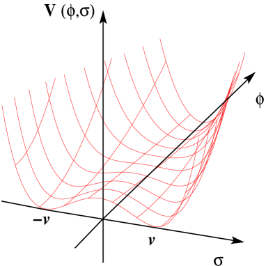
Figure 1: Potential for hybrid inflation.

The scalar potential for this kind of model looks like

$$V(\phi,\sigma)=\kappa(\sigma^{2}-v^{2})^{2}+\kappa^{\prime}\phi^{2}\sigma^{2}+V_{\phi}(\phi)\,;$$ (17)

during inflation $\phi^{2}\geq{2\kappa\over\kappa^{\prime}}v^{2}$ and the hybrid field is stabilized at the origin, so that the potential driving inflation, is

$$V(\phi,0)=V_{0}+V_{\phi}(\phi)\,,$$ (18)

with $V_{0}=\kappa v^{4}$; this expression has to be considered to compute the power spectrum and spectral index, as described in the previous section. Different hybrid inflationary models arise depending on the choice of $V_{\phi}(\phi)$. The typical shape of the hybrid inflationary potential is shown in Fig. 1, while some prediction for the spectral index on different models are shown in Table 1.

$1+V_{\phi}(\phi)/V_{0}$	$n-1$	$dn/d\log(k)$	Origin of the slope
$1-\frac{\lambda^{2}}{4\pi^{2}}\log\left({\sqrt{2}\lambda\phi\over Q}\right)$	${-1\over N+\frac{2\pi^{2}\phi_{c}^{2}}{\lambda^{2}M_{P}^{2}}}$	${-1\over\left(N+\frac{2\pi^{2}\phi_{c}^{2}}{\lambda^{2}M_{P}^{2}}\right)^{2}}$	1 loop for spont. broken susy
$1\pm\frac{1}{2}\frac{m^{2}_{\phi}}{V_{0}}\phi^{2}$	$\pm\frac{m^{2}_{\phi}M_{P}^{2}}{V_{0}}$	$0$	Susy breaking mass
$1\pm\beta\frac{\phi}{M_{P}}$	$-3\beta^{2}$	$0$	Susy breaking linear term
$1\pm\frac{\phi^{4}}{M_{P}^{4}}$	${12\over\frac{M_{P}^{2}}{2\phi_{c}^{2}}\mp N}$	${\mp 12\over\left(\frac{M_{P}^{2}}{2\phi_{c}^{2}}\mp N\right)^{2}}$	Sugra quartic term

Table 1: Various models of hybrid inflation and their prediction for the spectral index as a function of $N=-\log(k/k_{\mathrm{e}nd})$ and its derivative, assuming small field values. In the case of the simple linear term, $n-1$ is given by the full expression (11) since $\eta$ vanishes, but note that in supergravity generally, other contribution to the spectral index coming from higher order terms are usually present and can be larger than the one listed here [9].

We will describe in the following a couple of examples of hybrid inflation constructed within local supersymmetric theories. While supersymmetry is a vital ingredient at low energy for solving the hierarchy problem and stabilizing scalar masses, it could seem unnecessary to invoke it during inflation, especially since such symmetry is explicitely broken by the large effective cosmological constant responsible of the inflationary phase. It turns out anyway that supersymmetry brings many advantages also to inflationary model building, not only stabilizing the inflaton potential and its small parameters, but also providing many scalars as inflaton candidates, in particular the flat directions of the scalar potential. Moreover, if we assume low energy supersymmetry, as required by the hierarchy problem, it should certainly not be neglected at the large scale when inflation takes place.

However, we must not forget the fact that the inflationary vacuum energy breaks strongly supersymmetry and that supergravity corrections can play an important role [2].

2.1 Linear term hybrid inflation in supergravity

We will consider a model of inflation with superpotential [9]

$$W=\lambda T\left(M_{G}^{2}-\Sigma^{2}\right)+M_{S}^{2}(\beta+S)\;,$$ (19)

where $T,S$ and $\Sigma$ are chiral superfields. The second part of the superpotential is the Polonyi potential [10] and allows for supersymmetry breaking in the true vacuum with vanishing cosmological constant for $\beta\simeq(2-\sqrt{3})M_{P}$. $M_{S}$ is then the supersymmetry breaking scale, yielding the gravitino mass $m_{3/2}\simeq M_{S}^{2}/M_{P}$.

For global supersymmetry the scalar potential reads

$$V=\lambda^{2}|M_{G}^{2}-\Sigma^{2}|^{2}+4\lambda^{2}|T|^{2}|\Sigma|^{2}+M_{S}^{4}\;,$$ (20)

and it is of the hybrid inflationary type, even if perfectly flat along the $T$ and $S$ directions. A small curvature needed for the ‘slow roll’ along the $T$ direction is generated by many contributions, e.g. quantum corrections due to the loops of the $\Sigma$ particles [11], and also supergravity corrections.

For large $T$ and zero $\Sigma$ the dominant corrections to the potential give [9]

$$V(\phi)=\lambda^{2}M_{G}^{4}\left[1-2\sqrt{2}\xi\,{\beta\,\phi\over M_{P}^{2}}+{\phi^{4}\over 4M_{P}^{4}}+{\lambda^{2}\over 8\pi^{2}}\log\left({2\lambda^{2}\phi^{2}\over\mu^{2}}\right)+...\right].$$ (21)

where $\xi=M^{2}_{S}/(\lambda M^{2}_{G})\ll 1$, the first two terms come from supergravity corrections, and the last from one loop radiative corrections. The three terms in the potential compete and depending on the parameters $\lambda$, $\xi$ and $M_{G}$, different regimes can be realized. In all cases we have a viable model of hybrid inflation and we can fix one of the three parameters using the COBE normalization (8). Taking the supersymmetric scale $M_{S}$ to be in a phenomenologically acceptable range for low energy supersymmetry, $M_{S}=1.4\times 10^{10}\mbox{GeV}$ the parameter space is shown in Fig. 2.

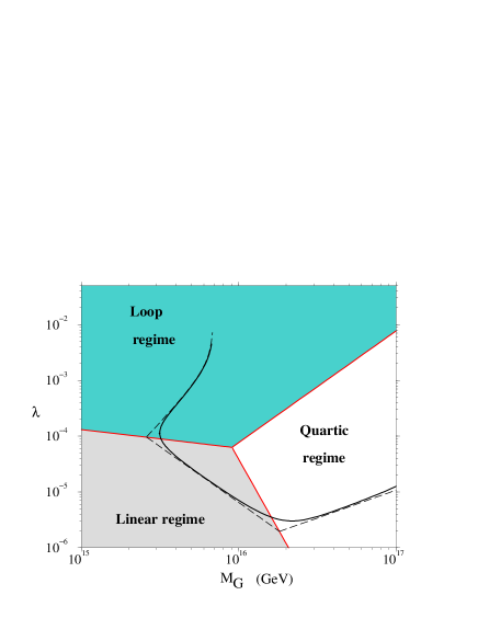
Figure 2: The three regimes of hybrid inflation: the loop regime, the linear regime and the quartic regime. The COBE normalization defines a curve (full line) in the $\lambda-M_{G}$ - plane for $M_{S}=1.4\times 10^{10}\,{\mathrm{G}eV}$. The dashed lines are obtained by keeping only the dominant term in the inflaton potential.

We see that the linear term dominates for small couplings and small $M_{G}$, and in that regime, from the COBE normalization (8), one obtains,

$${1\over 2\sqrt{150}\pi}{M_{S}^{2}\over\xi^{2}\beta M_{P}}=2.1\cdot 10^{-5}\;.$$ (22)

For $M_{S}\simeq 10^{10}\mbox{GeV}$, this gives $\xi\equiv M^{2}_{S}/(\lambda M_{G}^{2})\simeq 10^{-6}$. Note, that $\xi$ is the ratio of the gravitino masses in the true vacuum and in the inflationary phase. Since $\xi\ll 1$, slow-roll conditions are well satisfied for $\phi\simeq\phi_{c}$, and the spectral index is

$$n-1\simeq 3{\phi_{*}^{2}\over M_{P}^{2}}\leq 2.4\cdot 10^{-4}\;.$$ (23)

An inflationary phase dominated by a linear term is very interesting, since it gives a scale invariant spectrum to high accuracy. For standard hybrid inflation, on the contrary, one has $n\simeq 0.98$ [11]. Future satellite experiments may eventually be able to distinguish between these two regimes of hybrid inflation.

2.2 Mass term hybrid inflation

In case the inflaton transforms under a discrete or continuous symmetry, the linear term in the potential vanishes due to the symmetry and the lowest order term in the scalar potential lifting a flat direction is a mass term. We have in that case

$$V_{\phi}(\phi)={1\over 2}m^{2}\phi^{2}+...\,;$$ (24)

the dots are higher order terms who can become important at large field values.

Many models of this type, based on supersymmetric extensions of the Standard Model have been considered, starting with [12]. These models can have many different feature, depending on the particular implementation, see [2] for a review. For example, it has been recently realized, that in this class of models inflation can take place even at very low scales [13], softening the problem of realizing an inflationary epoch in the case of large extra-dimensions when the Planck mass is of order of the TeV scale.

Another interesting signature is the peculiar strong scale dependence of the spectral index, that appears in the case of large one loop quantum corrections to the inflaton potential [14]. Resumming those terms into the inflaton mass, we have in the potential the running mass $m(\phi)$:

$$V_{\phi}(\phi)={1\over 2}m^{2}(\phi)\phi^{2}+...\,;$$ (25)

so that, assuming the end of inflation is set by the beginning of fast roll, the spectral index is given by [15]

$${n(k)-1\over 2}\simeq\left.m^{2}(\phi)\right|_{k=aH}\,=s\left({k\over k_{cobe}}\right)^{c}-c\,;$$ (26)

where $s$ is an integration constant related to $\phi_{end}$, $c\propto{dm^{2}\over d\log(Q)}$ is proportional to the beta-function of the inflaton mass. We see that the scale dependence of the spectral index is in this case pretty strong (a power-law, but for the spectral index itself not the power spectrum !).

3 Comparison to observations

To obtain information about the primordial power spectrum and so on inflation, it is necessary to follow the perturbations from the inflationary to the present epoch and compare the processed spectrum to the observed one. Unfortunately, the evolution of the perturbations depends on the background cosmology and therefore on the cosmological parameters, i.e. the present Hubble parameter in units of $100\,\mathrm{km/s/Mpc},h$, the total energy density, $\Omega_{tot}$, the matter density $\Omega_{M}$ and the nature and composition of Dark Matter, the baryon density $\Omega_{b}$. It is for this reason not so straightforward to gain information on the primordial spectrum, without any assumption on the cosmology, or as it is usual said, without biases.

On large scales, below the size of the present horizon $\approx 3000\,\mathrm{Mpc}$ down to around $10\,\mathrm{Mpc}$, information on the power spectrum is provided by the CMBR anisotropies, on smaller scales, about $100$–$1\,\mathrm{Mpc}$ information comes instead from the visible matter power spectrum. During radiation dominance, due to the presence of pressure, the perturbations could not grow nor reach the instability regime and the dynamics was just an oscillation in the radiation plasma; the CMBR anisotropies are a snapshot of this period and they provide us with the cleanest signal. In fact, the dynamics of the plasma at that epoch is well understood and nowadays powerful computer codes like CMBFAST [16] are available to the scientific community to compute the CMBR anisotropies specifying the initial conditions and compare them to observations. On the other hand extracting the primordial power spectrum from the present matter power spectrum is more complicated since such perturbation reached the non-linear regime and underwent gravitational collapse.

3.1 CMBR observations

This year three new experimental measurements of the CMBR anisotropy were completed, providing the first view of three acoustic peaks in the CMBR spectrum [17, 18, 19].

The analysis of these data in order to extract the cosmological parameters have been performed, both for the single data sets, [20, 21, 22], and for the combined data [23], including also Maxima, Boomerang, Dasi and CBI [24]. All the analysis give results that are in good agreement with the general prediction of inflation:

• the position of the first peak of the CMBR is a direct measurement of the geometry of our universe and give a very clear indication that the spatial curvature is vanishing in accordance with the inflationary prediction; the total energy density as inferred from the CMBR only [23] is:

  $$\Omega_{tot}=1.06^{+0.13}_{-0.59}\,.$$ (27)

  As we can see, the precision of the measurement is not very high, due to degeneracies between the cosmological parameters, but imposing even weak biases on the values of some parameters or considering also large scale structure data, reduces strongly the uncertainties:

  $\Omega_{tot}$	Bias	Data and reference
  $1.04^{+0.11}_{-0.12}$	$h>0.45,\;\tau_{c}<0.4$	DMR & DASI [20]
  $0.90^{+0.18}_{-0.16}$	$0.4<h<0.9,\;\Omega_{M}>0.1,\;t_{0}>10$ Gyr	DMR & MAXIMA-I [21]
  $1.02^{+0.10}_{-0.10}$	$0.45<h<0.85,\;t_{0}>10$ Gyr	DMR & BOOMERANG [22]
  $1.00^{+0.06}_{-0.06}$	$h=0.72\pm 0.08$	PSCz & combined CMBR data [23]

  Table 2: Results for the total energy density of the universe with different biases and datasets. The errors correspond to 95% CL. For the third line [22], the error is obtained reading Fig. 4.

• it seems also that the curvature perturbations are compatible with a primordial spectrum gaussian [25] and adiabatic [26], so that we can conclude that the single field slow roll inflation does give a good fit to the present observations;

• a nearly scale invariant primordial spectrum ${\cal P}_{\cal R}(k)\propto k^{n-1}$ with $n\simeq 1$ is a good fit of the data, as we will see below in more detail;

• note also that the new CMBR observations are in very good agreement with other independent measurements, e.g. with the value of the baryon density obtained from Nucleosynthesis, $\Omega_{b}h^{2}=0.020\pm 0.002$ [27], and the determinations of the matter density from astrophysical observations [28]. The data seem also to prefer very low values for the hot dark matter density [23].

On the other hand, present data are much less powerful in discriminating between different models. For the spectral index we have in fact still a pretty wide allowed interval, containing most slow-rolling models, even after imposing constraints on the cosmological parameters:

$n$	Bias	Data and reference
$1.01^{+0.16}_{-0.11}$	$h>0.45,\;\tau_{c}<0.4$	DMR & DASI [20]
$0.99^{+0.14}_{-0.14}$	$0.4<h<0.9,\;\Omega_{M}>0.1\;,t_{0}>10$ Gyr, $\,\tau_{c}=0$	DMR & MAXIMA-I [21]
$0.97^{+0.18}_{-0.18}$	$0.45<h<0.85,\;t_{0}>10$ Gyr	DMR & BOOMERANG [22]
$0.93^{+0.13}_{-0.10}$	$h=0.72\pm 0.08$	PSCz & CMBR data [23]

Table 3: Results for the spectral index using different biases and datasets. The errors on $n$ correspond to 95% CL, and again for [22], the 95% CL interval is obtained from Fig. 4.

One of the problems of extracting $n$ is due to the degeneracy with the optical depth to the surface of last scattering $\tau_{c}$; such degeneracy can be reduced modeling reionization and estimating $\tau_{c}$ from the power spectrum itself [15].

In all these analysis, the primordial power spectrum is assumed to be a power-law with a constant spectral index. This is a reasonable assumption for many inflationary models, but it leaves unanswered an important question, i.e. how large is the scale dependence in $n$ allowed by the data. Two groups have studied this kind of constraints, but unfortunately have not yet up-dated their analysis to consider the latest data. In [15] the specific scale dependence of running mass models given by eq. (26) has been compared to observations and constraints on the values of the $s$ and $c$ parameters have been obtained, e.g. $-0.31\leq s\leq 0.21$ and $-0.21\leq c\leq 0.15$ at 95% CL. The analysis in [29, 30] relies instead in a Taylor expansion of the power spectrum as a function of $\log(k)$, truncated after the first derivative of the spectral index. Using not only CMBR and LSS data, but also linear matter power spectrum from Ly-$\alpha$ forest spectra, [30] obtained the strong constraint $-0.05\leq{dn\over d\log(k)}\leq 0.02$ at the 2$\sigma$ level.

4 Conclusions

We have seen that the single field inflationary paradigm is very successful in describing present observations, but unfortunately the precision of the present data is not yet sufficient to discriminate between the explicit models. To extract information on the primordial power spectrum from the CMBR is necessary to exploit all our knowledge of the cosmological parameters in order to reduce the degeneracies.

It is foreseeable that in the future a much better determination of the spectral index $n$ will be achieved, thanks both to more precise satellite experiments like MAP [31] and to the improvement of the measurements of the cosmological parameters by other astrophysical methods.

References

- [1] A. D. Linde, Particle Physics and Inflationary Cosmology, Harwood Academic (1990)
- [2] For a review and references, see D. H. Lyth and A. Riotto, Phys. Rept. 314 (1999) 1
- [3] C. L. Bennett et al., Astrophys. J. 464 (1996) L1
- [4] E. F. Bunn and M. White, Astrophys. J. 480 (1997) 6
- [5] A. R. Liddle and D. H. Lyth, Phys. Rept. 231 (1993) 1
- [6] M. Kamionkowski and A. H. Jaffe, astro-ph/0011329
- [7] P. Viana, astro-ph/0009492
- [8] A. D. Linde, Phys. Lett. B 259 (1991) 38
- [9] W. Buchmüller, L. Covi and D. Delépine, Phys. Lett. B 491 (2000) 183.
- [10] J. Polonyi, Budapest preprint KFKI-93 (1977)
- [11] G. Dvali, Q. Shafi and R. K. Schaefer, Phys. Rev. Lett. 73 (1994) 1886
- [12] L. Randall, M. Soljacic and A. Guth, Nucl. Phys. B 472 (1996) 377
- [13] G. German, G. Ross and S. Sarkar, Nucl. Phys. B 608 (2001) 423
- [14] E. D. Stewart, Phys. Rev. Lett. 391 (1997) 34, Phys. Rev. D 56 (1997) 2019; L. Covi and D. H. Lyth, Phys. Rev. D 59 (1999) 063515; L. Covi, D. H. Lyth and L. Roszkowski, Phys. Rev. D 60 (1999) 023509; G. German, G. Ross and S. Sarkar, Phys. Lett. B 469 (1999) 46
- [15] D. H. Lyth and L. Covi, Phys. Rev. D 62 (2000) 103504; L. Covi and D. H. Lyth, MNRAS 326 (2001) 885.
-
[16]
U. Seljak and M. Zaldarriaga, Astrophys. J. 469 (1996) 437;
http://physics.nyu.edu/matiasz/CMBFAST/cmbfast.html - [17] A. T. Lee et al., astro-ph/0104459
- [18] C. B. Netterfield et al., astro-ph/0104460
- [19] N. W. Halverson et al., astro-ph/0104489
- [20] C. Pryke et al., astro-ph/0104490
- [21] R. Stompor et al., astro-ph/0105062
- [22] P. de Bernardis et al., astro-ph/0105296
- [23] X. Wang, M. Tegmark and M. Zaldarriaga, astro-ph/0105091
- [24] S. Padin et al., Astrophys. J. 549 (2001) L1
- [25] J. H. P. Wu et al., astro-ph/0104248; S. F. Shandarin et al., astro-ph/0107136; M. G. Santos et al., astro-ph/0107588
- [26] D. Langlois and A. Riazuelo, Phys. Rev. D 62 (2000) 043504; R. Trotta, A. Riazuelo and R. Durrer, astro-ph/0104017
- [27] S. Burles, K. M. Nollett and M. S. Turner, Astrophys. J. 552 (2001) L1
- [28] M. S. Turner, astro-ph/0106035
- [29] S. Hannestad, S. Hansen and F. L. Villante, Astropart. Phys. 16 (2001) 137
- [30] S. Hannestad et al., astro-ph/0103047
- [31] http://map.gsfc.nasa.gov