Abstract

We calculate the cross section of a single inclusive gluon production in deep inelastic scattering at very high energies in the saturation regime, where the parton densities inside hadrons and nuclei are large and the evolution of structure functions with energy is nonlinear. The expression we obtain for the inclusive gluon production cross section is generated by this nonlinear evolution. We analyze the rapidity distribution of the produced gluons as well as their transverse momentum spectrum given by the derived expression for the inclusive cross section. We propose an ansatz for the multiplicity distribution of gluons produced in nuclear collisions which includes the effects of nonlinear evolution in both colliding nuclei.

I Introduction

At very high energies corresponding to very small values of Bjorken $x$ variable the density of partons in the hadronic and nuclear wave functions is believed to become very large reaching the saturation limit [1, 2, 3, 4]. In the saturation regime the growth of partonic structure functions with energy slows down sufficiently to unitarize the total hadronic cross sections. The gluonic fields in the saturated hadronic or nuclear wave function are very strong [5, 6]. A transition to the saturation region can be characterized by the saturation scale $Q_{s}^{2}(s)$, which is related to the typical two dimensional density of the partons’ color charge in the infinite momentum frame of the hadronic or nuclear wave function [4, 5, 6]. The saturation scale $Q_{s}^{2}(s)$ is an increasing function of energy $s$ and of the atomic number of the nucleus A [7, 8, 9, 10, 11, 12, 13, 14, 15, 16, 17]. At high enough energies or for sufficiently large nuclei the saturation scale becomes much larger than $\Lambda_{QCD}^{2}$ allowing for perturbative description of the scattering process at hand [4, 18]. The presence of intrinsic large momentum scale $Q_{s}$ justifies the use of perturbative QCD expansion even for such a traditionally non-perturbative observables as total hadronic cross sections.

Recently there has been a lot of activity devoted to calculating hadronic and nuclear structure functions in the saturation regime. The original calculation of quark and gluon distribution functions including multiple rescatterings without QCD evolution in a large nucleus was performed in [3]. The resulting Glauber-Mueller formula provided us with expressions for the partonic structure functions which reach saturation at small $Q^{2}$. McLerran and Venugopalan has argued in [4] that the large density of gluons in the partonic wave functions at high energy allows one to approximate the gluon field of a large hadron or nucleus by a classical solution of the Yang-Mills equations. The resulting gluonic structure functions has been shown to be equivalent to the Glauber-Mueller approach [5, 6, 19]. An important problem which still remained was the inclusion of quantum QCD evolution in this quasi-classical expression for the structure functions. The problem was equivalent to resummation of the multiple BFKL pomeron [20] exchanges. The evolution equation resumming leading logarithms of energy ($\alpha_{s}\ln s$) and the multiple pomeron exchanges was written in [7] using the dipole model of [8] and independently in [10] using the effective high energy lagrangian approach. The equation was written for the cross section of a quark-antiquark dipole scattering on a target hadron or nucleus, which, in turn can yield us the $F_{2}$ structure function of the target. The latter can be written as

$$F_{2}(x,Q^{2})=\frac{Q^{2}}{4\pi^{2}\alpha_{EM}}\int\frac{d^{2}rd\alpha}{2\pi}\,\Phi^{\gamma^{*}\rightarrow q{\bar{q}}}({\underline{r}},\alpha)\ d^{2}b\ N({\underline{r}},{\underline{b}},Y),$$ (1)

with $\Phi^{\gamma^{*}\rightarrow q{\bar{q}}}({\underline{r}},\alpha)$ the wave function of a virtual photon in deep inelastic scattering (DIS) splitting in a $q\bar{q}$ with transverse separation ${\underline{r}}$ and the fraction of photon’s longitudinal momentum carried by the quark $\alpha$. $\Phi^{\gamma^{*}\rightarrow q{\bar{q}}}({\underline{r}},\alpha)$ is a very well known function and could be found for instance in [7, 12, 18]. The quantity $N({\underline{r}},{\underline{b}},Y)$ has a meaning of a forward scattering amplitude of a dipole with transverse size $\underline{r}$ at impact parameter $\underline{b}$ with rapidity $Y$ on a target proton or nucleus normalized in such a way that the total cross section for the process is given by

$$\sigma^{q{\bar{q}}A}_{tot}\,=\,2\int d^{2}b\,N({\underline{r}},{\underline{b}},Y).$$ (2)

The evolution equation for $N$ closes only in the large-$N_{c}$ limit of QCD [10, 11] and reads [7, 8]

$$N({\underline{x}}_{01},{\underline{b}},Y)=-\gamma({\underline{x}}_{01},{\underline{b}})\,\exp\left[-\frac{4\alpha C_{F}}{\pi}\ln\left(\frac{x_{01}}{\rho}\right)Y\right]+\frac{\alpha C_{F}}{\pi^{2}}\int_{0}^{Y}dy\,\exp\left[-\frac{4\alpha C_{F}}{\pi}\ln\left(\frac{x_{01}}{\rho}\right)(Y-y)\right]$$

$$\times\int_{\rho}d^{2}x_{2}\frac{x_{01}^{2}}{x_{02}^{2}x_{12}^{2}}\,[2\,N({\underline{x}}_{02},{\underline{b}}+\frac{1}{2}{\underline{x}}_{12},y)-N({\underline{x}}_{02},{\underline{b}}+\frac{1}{2}{\underline{x}}_{12},y)\,N({\underline{x}}_{12},{\underline{b}}+\frac{1}{2}{\underline{x}}_{02},y)],$$ (3)

with the initial condition set by $\gamma({\underline{x}}_{01},{\underline{b}})$, which is the propagator of a dipole of size ${\underline{x}}_{01}$ at the impact parameter ${\underline{b}}$ through the target nucleus or hadron. $\gamma$ was taken to be of Mueller-Glauber form in [7]:

$$\gamma({\underline{x}}_{01},{\underline{b}}_{0})=e^{-{\underline{x}}_{01}^{2}Q_{0s}^{quark2}/4}-1,$$ (4)

where for a spherical nucleus [3, 19, 21]

$${\underline{x}}_{01}^{2}Q_{0s}^{quark2}\,=\,{\underline{x}}_{01}^{2}\ \frac{4\pi^{2}\alpha_{s}\sqrt{R^{2}-b^{2}}}{N_{c}}\,\rho\,xG(x,1/{\underline{x}}_{01}^{2}),$$ (5)

with $\rho=A/[(4/3)\pi R^{3}]$ the density of the atomic number $A$. The gluon distribution in Eq. (5) should be taken at the two-gluon order

$$xG(x,1/{\underline{x}}^{2})\ =\ \frac{\alpha_{s}C_{F}}{\pi}\,\ln\frac{1}{{\underline{x}}^{2}\mu^{2}},$$ (6)

with $\mu$ some infrared cutoff. The scale $Q_{0s}^{quark2}$ has the meaning of the quasi-classical quark saturation scale generated by multiple rescatterings prior to the inclusion of evolution. Eqs. (1) and (3) provide us with the $F_{2}$ structure function and the total cross section of DIS on a nucleus including all multiple BFKL pomeron exchanges (fan diagrams). In spite of several attempts to solve Eq. (3) analytically, which provided us with a well-understood high and low energy asymptotics for $N$ [7, 12, 11], the exact analytical solution is still to be found. There exist several numerical solutions to Eq. (3) demonstrating that at very high energies the amplitude $N$ goes to an independent of energy constant ($N\rightarrow 1$) thus unitarizing the total DIS cross sections [12, 13, 16, 17]. The numerical analyses also show that Eq. (3) does generate a momentum scale $Q_{s}$ which rapidly increases with energy. This scale justified the small coupling $\alpha_{s}$ expansion and helps avoid the problem of infrared instability of BFKL equation. An effort to calculate the NLO correction to Eq. (3) is currently under way [22].

Several other observables could be calculated in the framework of the saturation approach to hadronic and nuclear collisions. Of the exclusive observables diffractive (or, more precisely, elastic) cross section has been calculated in the quasi-classical limit in [23]. The evolution equation including multiple pomeron exchanges has been recently written for the cross section of single diffractive dissociation in [24].

In this paper we are interested in inclusive particle production cross sections. In the saturation framework these cross sections have been extensively studied at the classical level in DIS, proton–nucleus (pA) and nucleus–nucleus (AA) collisions. The inclusive gluon production cross section for pA and AA in the weak classical field limit (lowest order in perturbation theory without multiple rescatterings) has been calculated in [25], reproducing the result of Gunion and Bertsch [26]. In the strong field limit including all multiple rescatterings but no QCD evolution the gluon production cross section was calculated for pA in [19]. This result has been recently reproduced in [27, 28, 29]. The inclusive gluon production cross section for DIS was calculated in [21], with the resulting expression being slightly different from a straightforward generalization of the pA result of [19]. Finally an important problem for heavy ion physics is the calculation of the inclusive gluon production cross section in AA, which would provide us with the initial conditions for the possible formation of quark-gluon plasma. Numerical estimates of the related gluon multiplicities were performed in [30], while an analytical ansatz has been proposed in [31].

The problem of inclusion of nonlinear evolution in the inclusive cross sections received much less attention in the literature. The case of heavy flavor production in DIS with nonlinear evolution has been solved in [32]. The inclusive gluon production in DIS has been studied in [33, 34] using the AGK cutting rules [35] and $k_{T}$-factorization approach.

In this paper we calculate the single inclusive gluon production cross section in DIS including the effects of multiple rescatterings and nonlinear evolution of Eq. (3). We begin in Sect. II by reviewing the derivation of the formula for the single inclusive gluon production cross section in the quasi-classical approximation given in [21]. In the quasi-classical approximation the quantum evolution is not included since one is interested in resummation of multiple rescatterings [5, 19]. Each multiple rescattering of the produced gluon on a nucleon in the nucleus brings in a factor of $\alpha_{s}^{2}A^{1/3}$ and the quasi-classical approximation can be defined as resumming powers of this parameter [5, 18, 19, 31]. The result for gluon production cross section is shown in Eq. (12).

We continue in Sect. III by including the effects of nonlinear dipole evolution from Eq. (3) in the expression for the cross section. The philosophy of our approach is similar to [7]. We first construct a classical Glauber-Mueller–type expression for the inclusive cross section and then use it as our starting point for including dipole evolution. We are working in the rest frame of the target, which allows to consider the quantum evolution in energy as happening only in the wave function of the incoming $q{\bar{q}}$ pair [7, 10]. In Sect. IIIA we analyze the evolution preceding the emission of the gluon that we measure in the final state. This evolution corresponds to emission of gluons with larger (harder) light cone component of momentum than the one carried by the gluon that we trigger. We show that this early evolution can only be linear (single pomeron exchange) leading to creation of the dipole in which our measured gluon is emitted. This conclusion is in agreement with the prediction of AGK cutting rules for inclusive cross section [33, 34, 35, 36]. In Sect. IIIB we proceed by analyzing the emissions of the gluons which are softer than the measured one. We demonstrate that the effect of these later emissions can be incorporated in the inclusive cross section by replacing the Glauber-Mueller exponents in Eq. (12) with the evolved forward amplitudes of a gluon (adjoint) dipole scattering on the target. The final expression for inclusive gluon production cross section in DIS is given by Eq. (36) in Sect. IIIC which is the main result of this paper.

We begin analyzing the cross section of Eq. (36) in Sect. IV by observing that in the case of a very large nucleus corresponding to zero momentum transfer in each of the exchanged pomerons it can be rewritten in a factorized form as a convolution of two functions with Lipatov’s effective vertex inserted in the middle (see Eq. (45)). In this form it almost agrees with the expression derived by Braun in [34] using the AGK rules and pomeron fan diagram approach (see Eq. (10) in [34]). To obtain the expression given in [34] from our Eq. (45) one has to replace in it the evolved forward amplitude of an adjoint dipole on the target nucleus $N_{G}$ by the similar amplitude for the fundamental dipole $N$. While the difference seems minor in the weak field limit given by the linear evolution equations, it becomes much more profound in the transition to the saturation region where the quantities $N_{G}$ and $N$ obey different evolution equations while approaching the same high energy asymptotics. In Sect. V we study the transverse momentum spectrum and energy dependence of the obtained cross section. We observe that while at very large $k_{\perp}$ the cross section exhibits the usual $1/k_{\perp}^{4}$ behavior it softens to $1/k_{\perp}^{2}$ in the small $k_{\perp}\sim Q_{s}$ region similarly to the quasi-classical cross sections of [19, 21]. The rapidity distribution of the produced gluons may have a maximum which position is determined by the values of the produced gluon’s momentum $k_{\perp}$ and photon’s virtuality $Q$ (see Fig. 7).

We conclude in Sect. VI by discussing the general principles of inclusion of nonlinear evolution in the cross sections for various inclusive processes. We present an ansatz for the multiplicity distribution of the produced gluons in nucleus–nucleus collisions (AA) including the effects of nonlinear evolution in both colliding nuclei.

II Inclusive Cross Section in the Quasi–Classical Approximation

In this Section we will review the derivation of the single inclusive gluon production cross section in DIS from [21] in the quasi-classical approximation developed in [19]. The gluon production cross section in DIS can be rewritten as

$$\frac{d\sigma^{\gamma^{*}A\rightarrow q{\bar{q}}GX}_{incl}}{d^{2}k\,dy}\,=\,\frac{1}{2\pi^{2}}\,\int\,d^{2}x_{01}\,d\alpha\,\Phi^{\gamma^{*}\rightarrow q\bar{q}}({\underline{x}}_{01},\alpha)\,\frac{d{\hat{\sigma}}^{q{\bar{q}}A}_{incl}}{d^{2}k\,dy}({\underline{x}}_{01}),$$ (7)

where $d{\hat{\sigma}}^{q{\bar{q}}A}_{incl}/d^{2}k\,dy({\underline{x}}_{01})$ is the gluon production cross section for the scattering of a dipole of transverse size ${\underline{x}}_{01}={\underline{x}}_{0}-{\underline{x}}_{1}$ on the target. We want to calculate this observable including all multiple rescatterings of the $q\bar{q}$ pair and the produced gluon on the nucleons in the target nucleus. In the quasi-classical approximation each rescattering happens via one or two gluon exchanges with the nucleon [19]. We assume that the initial quark-antiquark pair is moving in the “+” light cone direction. The diagrams contributing to the gluon production cross section in the $A_{+}=0$ light cone gauge are shown in Fig. 1.

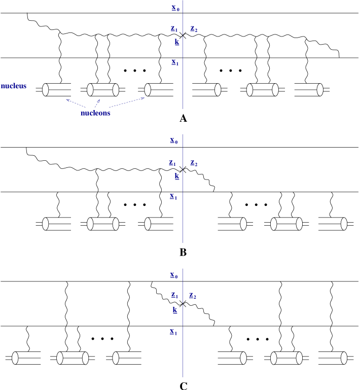
FIG. 1.: Gluon production in DIS in the quasi-classical approximation. The produced gluon may be emitted either off the quark or off the antiquark lines both in the amplitude and in the complex conjugate amplitude. Only one connection is shown.

Similar to [19, 21, 27, 28, 29, 31] the gluon emission can happen via two possible scenarios: the incoming dipole may have the gluon fluctuation in its wave function by the time it hits the target or the gluon may be emitted after the dipole interacts with the target. Even with all the multiple rescatterings the interaction with the target is instantaneous compared to the typical emission time of the gluon [19]. We thus may denote the interaction time $\tau\equiv x_{+}=0$. If the gluon emission time in the amplitude is $\tau_{1}$ and in the complex conjugate amplitude is $\tau_{2}$ than the following classification of diagrams in Fig. 1 is possible. The graph in Fig. 1A corresponds to the case when $\tau_{1}<0$ and $\tau_{2}<0$, while the diagram in Fig. 1B reflects the $\tau_{1}<0$, $\tau_{2}>0$ case. A “mirror image” diagram should be added to Fig. 1B describing the $\tau_{1}>0$, $\tau_{2}<0$ case. The late emission $\tau_{1}>0$, $\tau_{2}>0$ scenario is represented in Fig. 1C. The produced gluon line can start off either quark or antiquark lines both in the amplitude and in the complex conjugate amplitude in Fig. 1. We are going to sum over all possible emissions while only one case is shown in Fig. 1.

To calculate the diagrams in Fig. 1 we will be working in transverse coordinate space with the intent to perform a Fourier transform into momentum space in the end. Thus the produced gluon has different transverse coordinates in the amplitude and in the complex conjugate amplitude (${\underline{z}}_{1}$ and ${\underline{z}}_{2}$). The dipole consists of the quark at ${\underline{x}}_{0}$ and an antiquark at ${\underline{x}}_{1}$. Due to real-virtual cancellations only the diagrams where the nucleons interact with the produced gluon survive in Fig. 1A [19]. The square of the gluon’s propagator could be easily calculated to give [19]

$$e^{-({\underline{z}}_{1}-{\underline{z}}_{2})^{2}Q_{0s}^{2}/4}$$ (8)

with

$${\underline{x}}^{2}Q_{0s}^{2}\,=\,{\underline{x}}^{2}\ \frac{8\pi^{2}\alpha_{s}N_{c}\sqrt{R^{2}-b^{2}}}{N^{2}_{c}-1}\,\rho\,xG(x,1/|{\underline{x}}|^{2}).$$ (9)

The scale $Q_{0s}^{2}$ has the meaning of the gluon saturation scale in the quasi-classical (no evolution) approximation and is different from the quark saturation scale of Eq. (5) by the Casimir operator. In Fig. 1B only the interactions with the gluon line and the antiquark are allowed. Performing the calculation along the lines of Appendix A in [19] and adding the “mirror” contribution one obtains

$$-e^{-({\underline{z}}_{1}-{\underline{x}}_{1})^{2}Q_{0s}^{2}/4}-e^{-({\underline{z}}_{2}-{\underline{x}}_{0})^{2}Q_{0s}^{2}/4}.$$ (10)

The minus sign in Eq. (10) is due to the fact that the gluon is emitted after the interaction on one side of the cut in Fig. 1B. Finally the interactions with the nucleons shown in Fig. 1C would have canceled if we were considering proton-nucleus (or, more precisely, quark-nucleus) collisions as it was done in [19]. However, in the DIS case at hand the quark and antiquark originate from a virtual photon and thus have to be in the color singlet initial state on both sides of the cut. This condition was not imposed in pA [19, 29] where the color of the interacting quark was assumed to be randomized by the non-perturbative “intrinsic” quarks and gluons in the proton’s wave function [37]. Therefore, unlike the pA case moving an exchanged gluon line across the cut in DIS would modify the color factor of the diagram and thus real-virtual cancellation would not happen. A calculation of the interactions gives

$$e^{-({\underline{x}}_{0}-{\underline{x}}_{1})^{2}Q_{0s}^{2}/4}$$ (11)

for the diagram in Fig. 1C.

To obtain the final answer we now have to combine the terms from Eqs. (8), (10) and (11), multiply by the amplitude of gluon’s emission in the original dipole while keeping in mind that the amplitudes in Fig. 1 are slightly different for different connections of the gluon to the $q\bar{q}$ pair. We then should Fourier transform the expression into momentum space. The final result for the single inclusive gluon production cross section of dipole-nucleus scattering in the quasi–classical approximation reads

$$\frac{d{\hat{\sigma}}^{q{\bar{q}}A}_{incl}}{d^{2}k\,dy}({\underline{x}}_{01})\,=\,\frac{\alpha_{s}C_{F}}{\pi^{2}}\,\frac{1}{(2\pi)^{2}}\,\int\,d^{2}b\,d^{2}z_{1}\,d^{2}z_{2}\,e^{-i{\underline{k}}\cdot({\underline{z}}_{1}-{\underline{z}}_{2})}\,\sum_{i,j=0}^{1}(-1)^{i+j}\frac{{\underline{z}}_{1}-{\underline{x}}_{i}}{|{\underline{z}}_{1}-{\underline{x}}_{i}|^{2}}\cdot\frac{{\underline{z}}_{2}-{\underline{x}}_{j}}{|{\underline{z}}_{2}-{\underline{x}}_{j}|^{2}}$$

$$\times\left(e^{-({\underline{x}}_{i}-{\underline{x}}_{j})^{2}Q_{0s}^{2}/4}-e^{-({\underline{z}}_{1}-{\underline{x}}_{j})^{2}Q_{0s}^{2}/4}-e^{-({\underline{z}}_{2}-{\underline{x}}_{i})^{2}Q_{0s}^{2}/4}+e^{-({\underline{z}}_{1}-{\underline{z}}_{2})^{2}Q_{0s}^{2}/4}\right)$$ (12)

where ${\underline{b}}=({\underline{x}}_{0}+{\underline{x}}_{1})/2$ is the dipole’s impact parameter. Together Eqs. (7) and (12) give us the inclusive gluon production cross section in DIS in the quasi–classical approximation as derived in [21].

III Inclusion of Evolution Effects

We are now going to include quantum evolution into Eq. (12). We begin in Sect. IIIA by discussing the evolution preceding the emission of the measured gluon, and continue in Sect. IIIB by analyzing the subsequent evolution. The final expression is derived in Sect. IIIC.

A Emission of Harder Gluons

Let us explore how the emission of gluons with the light cone “plus” component of the momentum much larger than that of the measured gluon modify the inclusive cross section. For simplicity we first consider an emission of a single extra gluon. The diagrams relevant for real emission of this extra gluon are shown in Fig. 2. Since we are interested in the large-$N_{c}$ dipole evolution all gluons are represented by double quark lines. Notations are explained in Fig. 2A. The incoming original dipole of transverse size ${\underline{x}}_{01}={\underline{x}}_{0}-{\underline{x}}_{1}$ emits a (harder) gluon with transverse coordinate ${\underline{x}}_{2}$. Then the measured gluon ($\#3$) is emitted in one of the color dipoles formed by the emission of gluon $\#2$. Since we are interested in keeping this gluon’s transverse momentum fixed in the final state its transverse coordinates are different on each side of the cut (${\underline{x}}_{3}$ and ${\underline{x}}_{3^{\prime}}$). Emission in the lower dipole only is shown in Fig. 2. Emission in the upper dipole is completely analogous and could be obtained from Fig. 2 by switching gluons $2$ and $3$.

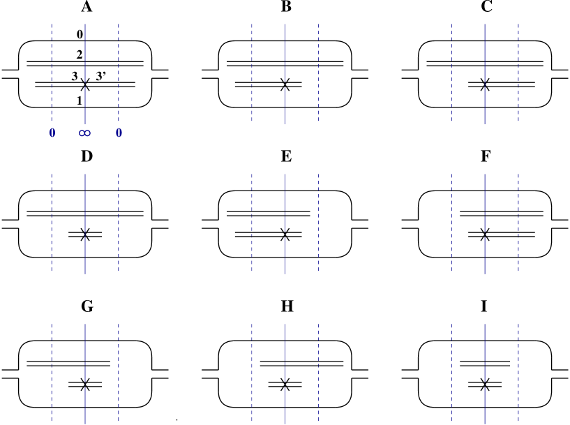
FIG. 2.: Emission of a harder gluon in the dipole evolution. Gluons are denoted by double lines in the large $N_{c}$ limit. The produced gluon is marked by a cross.

The gluon lines in Fig. 2 can connect to either quark or antiquark lines in the dipoles off which they are emitted both in the amplitude and in the complex conjugate amplitude. This is shown in Fig. 2 by not connecting the gluon lines to any of the quark line specifically. For instance the gluon $\#2$ can be emitted off the quark line $0$ and off the antiquark line $1$, which is demonstrated by drawing gluon $\#2$ directly between those quark lines. This notation is the same as the one used in [9, 24]. The interactions with the target are not shown explicitly in Fig. 2. Instead we mark with a dashed vertical line in Fig. 2 the moment in light cone time $\tau=0$ when the multiple rescatterings of Fig. 1 occur (see Fig. 2A). Of course the interactions may happen both in the amplitude and in the complex conjugate amplitude. The solid vertical line in Fig. 2 denotes the final state corresponding to $\tau=\infty$.

The measured gluon $\#3$ is much softer than the gluon $\#2$, $k_{3+}\ll k_{2+}$, while their transverse momenta are not ordered. Thus the lifetime of the gluon $\#2$ is much longer than that of gluon $\#3$. Therefore it seems natural that in all the diagrams considered in Fig. 2 the gluon $\#2$ is emitted before gluon $\#3$ on both sides of the cut. However the graphs in Fig. 2 do not cover all the diagrams which need to be considered. There is another set of diagrams, predominantly with the virtual emission of gluon $\#2$, some of which are shown in Fig. 4, that could be important for gluon production at this order. We are going to first analyze the diagrams in Fig. 2, which would allow us to understand which ones of the diagrams omitted in Fig. 2 should be considered.

The transverse momentum $\underline{k}$ and rapidity $y$ of the measured gluon $\#3$ are kept fixed, while the transverse momentum and rapidity of the other emitted gluon are integrated over. In the spirit of the leading logarithmic evolution integration over the rapidity of the gluon $\#2$ is supposed to give us the factor of $\ln 1/x$ with $x$ the Bjorken $x$ variable, or, equivalently, a factor of total rapidity interval $Y$. This factor would make up for the suppression by the power of coupling constant $\alpha_{s}$ that we have introduced by emitting that gluon. Now we are going to demonstrate that this enhancement does not happen in Figs. 2E–2I. That implies that the diagrams in Figs. 2E–2I do not give a leading logarithmic contribution and could be neglected as subleading.

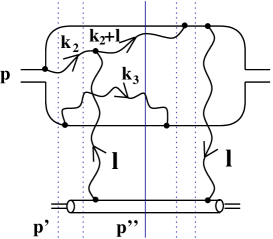
FIG. 3.: One of the diagrams contributing to the class of graphs represented by Fig. 2E.

Let us calculate the diagram in Fig. 3, which is one of the graphs represented by Fig. 2E. The diagrams in Fig. 2 are understood to be in the light cone perturbation theory (LCPT) [38], which has been used in the original construction of the QCD dipole model [8]. Therefore we will use the diagrammatic rules of LCPT in evaluating the graph Fig. 3. We are working in the frame where the quarks in the original dipole have large “$+$” components of their momenta while the nucleons in the nucleus have large “$-$” momentum components. Though only one rescattering is depicted in Fig. 3 our conclusions will be easy to generalize to include multiple Glauber rescatterings of Fig. 1. The intermediate states are denoted by vertical dotted lines in Fig. 3. In estimating the energy denominators of the intermediate states at $\tau>0$ one should remember that the “$-$” component of the nucleon’s momentum also changes. According to the rules of LCPT the “$-$” component of the final state should be equal to the “$-$” component of the initial (incoming) state [38]. Thus one requires that for the diagram in Fig. 3 the following condition should be satisfied

$$p^{\prime\prime}_{-}+\frac{({\underline{k}}_{2}+{\underline{l}})^{2}}{2k_{2+}}+\frac{{\underline{k}}_{3}^{2}}{2k_{3+}}\,=\,p^{\prime}_{-},$$ (13)

where we have used that for exchanged Coulomb gluons $l_{-}=0$ [5, 19]. Using Eq. (13) in evaluating, for instance, the energy denominator of the rightmost intermediate state in Fig. 3 yields [38]

$$\frac{1}{p^{\prime\prime}_{-}-p^{\prime}_{-}}\,=\,\frac{1}{-\frac{({\underline{k}}_{2}+{\underline{l}})^{2}}{2k_{2+}}-\frac{{\underline{k}}_{3}^{2}}{2k_{3+}}}\,\approx\,\frac{1}{-\frac{{\underline{k}}_{3}^{2}}{2k_{3+}}}.$$ (14)

We have used the fact that $k_{3+}\ll k_{2+}$ in the last approximation in Eq. (14). The rule for calculating the diagrams in Fig. 2 could be formulated as follows: the energy denominators for intermediate states with $\tau>0$ should consist of the sum of the “$-$” momenta components of all the intermediate gluons in the state minus the “$-$” momenta components of all the gluons in the final state. (Note that according to the rules of LCPT the “$-$” momenta components are not conserved at the vertices and all intermediate lines are on mass shell [38].)

Using the outlined strategy one can show that the contribution of the diagram in Fig. 3 is proportional to

$$\int_{k_{3+}}^{p_{+}}dk_{2+}\sum_{\lambda_{2},\lambda_{3}}\,\frac{{\underline{\epsilon}}_{2}^{\lambda_{2}}\cdot{\underline{k}}_{2}\,{\underline{\epsilon}}_{2}^{\lambda_{2}}\cdot({\underline{k}}_{2}+{\underline{l}})\,({\underline{\epsilon}}_{3}^{\lambda_{3}}\cdot{\underline{k}}_{3})^{2}}{({\underline{k}}_{3}^{2})^{3}\,{\underline{k}}_{2}^{2}\,k_{2+}^{2}}\,=\,\int_{k_{3+}}^{p_{+}}dk_{2+}\frac{{\underline{k}}_{2}\cdot({\underline{k}}_{2}+{\underline{l}})}{({\underline{k}}_{3}^{2})^{2}\,{\underline{k}}_{2}^{2}\,k_{2+}^{2}}\,\approx\,\frac{{\underline{k}}_{2}\cdot({\underline{k}}_{2}+{\underline{l}})}{({\underline{k}}_{3}^{2})^{2}\,{\underline{k}}_{2}^{2}\,k_{3+}}\,\sim\,\frac{1}{k_{3+}}$$ (15)

with $p_{+}$ a large momentum of one of the quarks in the original dipole ($k_{3+}\ll p_{+}$). As can be seen from Eq. (15) the diagram in Fig. 3 does not contain any logarithms of energy. It should be compared to the contribution of, for instance, diagram in Fig. 2A, which is proportional to

$$A\,\sim\,\int_{k_{3+}}^{p_{+}}dk_{2+}\frac{1}{k_{2+}\,k_{3+}}\,=\,\frac{1}{k_{3+}}\,\ln\frac{p_{+}}{k_{3+}}.$$ (16)

This diagram is enhanced by extra logarithm of energy (or, equivalently, an extra factor of rapidity) and should be included in our leading logarithmic analysis. In the same approximation the diagram in Fig. 3 is subleading since it does not have a logarithm of energy in it. Similar calculations can be carried out for all the diagrams in Fig. 2E showing that they are subleading and should be neglected. Finally the same conclusion will be reached if one analyzes all diagrams in Figs. 2E–2I : they do not bring in an extra logarithm of energy and therefore must be neglected.

Here we would like to remind the reader about the approximation we are using. It is the same approximation as outlined in [7] for the calculation of total DIS cross section. The (nonlinear) quantum evolution resums the powers of $\alpha_{s}N_{c}Y$ and is a function of this parameter [8]. ($Y$ is the rapidity variable.) At the same time we are interested in resumming multiple rescatterings, which also bring in extra powers of $\alpha_{s}$ [5, 19, 31]. The multiple rescatterings are limited to two gluon exchanges with each nucleon. Thus the actual parameter which is being resummed by multiple rescatterings is $\alpha_{s}^{2}A^{1/3}$ [5, 19, 31]. Therefore the combination of leading logarithmic large-$N_{c}$ evolution and Glauber-Mueller multiple rescatterings resums all powers of both $\alpha_{s}N_{c}Y$ and $\alpha_{s}^{2}A^{1/3}$ in the cross sections. From this point of view the diagrams in Figs. 2E–2I are suppressed by an extra power of $\alpha_{s}N_{c}$ not enhanced by an extra power of $Y$.

We have proven that of all graphs in Fig. 2 only diagrams in Figs. 2A–2D contribute. Based on this information one may conjecture that the evolution preceding the emission of the measured gluon consists of gluons emitted before interaction both in the amplitude and in the complex conjugate amplitude. To complete the proof of this statement we have to consider a whole class of diagrams where the line of gluon $\#2$ is shorter or of the same length as the line of gluon $\#3$. These diagrams include virtual diagrams where gluon $\#2$ is not present in the final state. Many of these diagrams are also subleading, similar to Figs. 2E–2I. This can be seen by performing the analysis outlined above and using the rule presented in the Appendix of [9] for calculation of virtual contributions. At the end we are left with the diagrams shown in Fig. 4, each of which gives a leading logarithmic contribution. Not all of the diagrams in Fig. 4 are symmetric with respect to horizontal (left-right) mirror reflections. Therefore one should add mirror images to diagrams A–D, F–P which will be denoted by primes (e.g. A’, B’, etc.). We note that due to momentum conservation the gluon $\#2$ can be emitted only off the quark lines $0$ and $1$ in the original dipole. Therefore moving part or all of gluon $\#2$ across the cut does not change the transverse coordinate (and, therefore, transverse momentum) structure of the diagrams. Using the cancellation of final state interactions demonstrated in [9] we observe that in Fig. 4

$$B+C\,=\,B^{\prime}+C^{\prime}\,=\,0$$ (18)

$$D+E+D^{\prime}=\,0$$ (19)

$$H+I\,=\,H^{\prime}+I^{\prime}\,=\,0$$ (20)

$$J+K\,=\,J^{\prime}+K^{\prime}\,=\,0$$ (21)

$$L+M+N\,=\,L^{\prime}+M^{\prime}+N^{\prime}\,=\,0$$ (22)

$$P+Q+P^{\prime}\,=\,0.$$ (23)

We are left only with the diagrams A, F, G, O and their mirror images A’, F’, G’, O’ in Fig. 4.

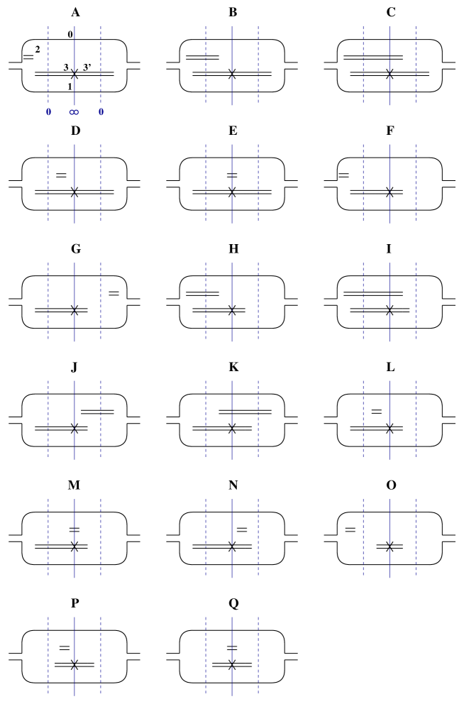
FIG. 4.: Another set of graphs contributing to emission of a harder gluon in the dipole evolution.

Combining the results of the analyses of the diagrams in Figs. 2 and 4 we conclude that only the diagrams where gluon $\#2$ is either emitted or both emitted and absorbed before the interaction at $\tau<0$ survive. The non-vanishing diagrams are graphs A–D in Fig. 2 and A, F, G, O, A’, F’, G’, O’ in Fig. 4. One can easily check that these diagrams add up to give us one rung of the linear dipole (or, equivalently, BFKL) evolution. The diagrams A–D in Fig. 2 provide us with the real part of the dipole kernel, splitting the original dipole $01$ in two, in one of which we continue the evolution by emitting the measured gluon $\#3$. Diagrams A, F, G, O, A’, F’, G’, O’ of Fig. 4 yield us with virtual corrections to the same process.

Now we are in a position to generalize our conclusions to the case of many harder gluons in the virtual photon’s wave function. The evolution preceding the emission of the measured gluon is the usual early-time dipole evolution leading to creation at early times (before the interaction, $\tau<0$) of the dipole in which the measured gluon is emitted. The effect of this evolution is to modify the probability of finding this dipole in the virtual photon’s wave function.

This preceding evolution can only be linear. This can be understood by analyzing diagrams A–D in Fig. 2. Real emissions in the dipole model may lead to branching of one dipole evolution into two simultaneous evolutions, being thus equivalent to triple pomeron vertices in the traditional language [7, 8, 13, 39]. For instance, in Figs. 2A–2D there could in principle be some subsequent evolution in the dipole $02$ leading to creation of many dipoles which would interact with the target. The evolution may also lead to creation of dipoles at late times ($\tau>0$). However all these emissions and interactions would not modify the momentum of the gluon that we measure, since they happen in a different dipole isolated from ours in the large-$N_{c}$ limit. Therefore one can show that all these interactions would cancel via real–virtual cancellations: first one can show the cancellation of Coulomb gluon exchanges similarly to some of the cancellations in Sect. II and then the cancellation of evolution in dipole $02$ follows due to probability conservation (see [8, 9]). This can be done for any graph where the evolution branches into two with the emitted gluon being produced by one of the subsequent evolutions. We therefore conclude that the early evolution is linear. This conclusion is similar to what one would obtain applying AGK cutting rules to the process [33, 34, 35, 36]. We will return to this similarity in the next Section.

To include the preceding evolution into the gluon production cross section of Eq. (7) one should thus substitute

$$\int\,d^{2}x_{01}\,d\alpha\,\Phi^{\gamma^{*}\rightarrow q\bar{q}}({\underline{x}}_{01},\alpha)\,\rightarrow\,\int d^{2}r\,d\alpha\,\Phi^{\gamma^{*}\rightarrow q{\bar{q}}}({\underline{r}},\alpha)\ d^{2}B\ n({\underline{r}},{\underline{x}}_{01},{\underline{B}}-{\underline{b}},Y-y)\,\frac{d^{2}x_{01}}{2\pi x^{2}_{01}}\,$$ (24)

where $n({\underline{r}},{\underline{x}}_{01},{\underline{b}},Y)$ is the number density of dipoles of size $x_{01}$ at an impact parameter ${\underline{b}}$ where the momentum fraction of the softest of the two gluons involved in making up the dipole is greater than $e^{-Y}$. The quantity $n({\underline{r}},{\underline{x}}_{01},{\underline{b}},y)$ was defined in [8] and was shown to satisfy the linear evolution equation equivalent to BFKL. The solution of that equation gives [8]

$$\int d^{2}B\,n({\underline{r}},{\underline{x}}_{01},{\underline{B}},Y)\ =\ \int\frac{d\lambda}{\pi i}\,e^{{\overline{\alpha}_{s}}\chi(\lambda)Y}\,\left(\frac{r}{x_{01}}\right)^{2\lambda},$$ (25)

where $\chi(\lambda)$ is the eigenvalue of the BFKL kernel [20] defined as

$$\chi(\lambda)\,=\,2\,\psi(1)-\psi(1-\lambda)-\psi(\lambda)$$ (26)

and

$${\overline{\alpha}_{s}}\,=\,\frac{\alpha_{s}N_{c}}{\pi}.$$ (27)

Integration in Eq. (25) runs along a straight line parallel to imaginary axis to the right of all the singularities of the integrand. In Eq. (24) $Y$ is the total rapidity interval of the DIS process while the measured emitted gluon is located at rapidity $y$.

B Emission of Softer Gluons

In the previous Subsection we have understood how to include the evolution of the harder gluons in the virtual photon’s wave function. Here we will address the question of how to include the evolution of gluons with the light cone component of their momenta being softer than the measured one. For instance, in Fig. 2 after being emitted the measured gluon splits the dipole $02$ into two off-forward dipoles. The dipoles are off-forward because the transverse coordinate of the measured gluon is not the same in the amplitude and in the complex conjugate amplitude. Nevertheless there could still be dipole-like evolution in each of these two dipoles. More gluons with light cone components of their momenta much smaller than $k_{3+}$ can be produced and these gluons can interact with the target as well.

We claim that in order to include the effects of this quantum evolution (in the leading logarithmic approximation) into Eq. (12) one has to substitute

$$1-e^{-{\underline{x}}^{2}Q_{0s}^{2}({\underline{b}})/4}\,\,\longrightarrow\,\,N_{G}({\underline{x}},{\underline{b}},y)$$ (28)

for all the Glauber exponents in it. The quantity $N_{G}({\underline{x}},{\underline{b}},y)$ is the forward amplitude of a gluon dipole scattering on the target. This quantity is similar to $N({\underline{x}},{\underline{b}},y)$ except the initial state for $N_{G}$ consists of a pair of gluons in the color singlet state instead of a quark-antiquark pair. The normalization of $N_{G}$ is analogous to Eq. (2). In the large-$N_{c}$ limit an adjoint (gluon) dipole can be decomposed into two fundamental (quark) dipoles. Therefore the scattering amplitude of a single adjoint dipole on a target nucleus in the large-$N_{c}$ approximation is equivalent to the scattering of two fundamental dipoles on the same target. One can thus conclude that

$$N_{G}({\underline{x}},{\underline{b}},y)\,=\,2\,N({\underline{x}},{\underline{b}},y)-N^{2}({\underline{x}},{\underline{b}},y).$$ (29)

The evolution equation for $N_{G}({\underline{x}},{\underline{b}},y)$ can be obtained by inverting Eq. (29) to express $N$ in terms of $N_{G}$

$$N({\underline{x}},{\underline{b}},y)\,=\,1-\sqrt{1-N_{G}^{2}({\underline{x}},{\underline{b}},y)}$$ (30)

and by substituting Eq. (30) into Eq. (3).

One can see right away that without evolution ($y=0$) Eq. (28) turns into equality (see, for instance, [3])

$$N_{G}({\underline{x}},{\underline{b}},0)\,=\,1-e^{-{\underline{x}}^{2}Q_{0s}^{2}({\underline{b}})/4}.$$ (31)

Our goal now is to prove that the substitution of Eq. (28) does correctly incorporate the effects of subsequent evolution in the gluon production cross section. As we now know the preceding quantum evolution happens only at $\tau<0$ and does not interfere with the subsequent one. Similarly to Sect. II one should consider four different cases, corresponding to different emission times of the measured gluon in the amplitude ($\tau_{1}$) and in the complex conjugate amplitude ($\tau_{2}$). The four cases are: $(1)\,\tau_{1}<0,\tau_{2}<0;\,\,(2)\,\tau_{1}<0,\tau_{2}>0;\,\,(3)\,\tau_{1}>0,\tau_{2}<0;\,\,(4)\,\tau_{1}>0,\tau_{2}>0$.

Let us first consider case $(1)$. In the quasi-classical case of Eq. (7) it gave us the exponent in Eq. (8). According to Eq. (28) we now have to prove that evolution replaces that exponent with $1-N_{G}\left({\underline{z}}_{1}-{\underline{z}}_{2},\frac{1}{2}({\underline{z}}_{1}+{\underline{z}}_{2}),y\right)$. That means that the gluons in the subsequent evolution connect only to the emitted gluon line mimicking the scattering amplitude of a gluon dipole of size ${\underline{z}}_{1}-{\underline{z}}_{2}$ on a nucleus.

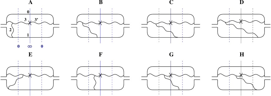
FIG. 5.: Diagrams including one softer gluon produced after the emission of the measured gluon.

To prove that the gluons in the subsequent evolution connect only to the gluon line of the measured gluon let us again consider a simple case when we add one more gluon emission to the quasi-classical diagrams of Fig. 1. Different from the previous Subsection the extra gluon’s light cone momentum should be much softer that the measured gluon’s one. To prove the cancellation of all the diagrams where the extra soft gluon interacts with the quark lines it is sufficient to consider graphs presented in Fig. 5. There after emitting the measured gluon $\#3$ we include and extra emission of a softer gluon $\#2$ ($k_{2+}\ll k_{3+}$). All the other relevant diagrams could be obtained by vertical and horizontal reflections of the graphs in Fig. 5. In Fig. 5 we kept only the diagrams where the emission of gluon $\#2$ is enhanced by a logarithm of energy leaving out all the subleading ones similar to how it was done in obtaining Fig. 4. The diagrams where the soft gluon ($\#2$) is both emitted and absorbed by quark lines are easily canceled by real-virtual cancellations [8, 9, 24] and need not be considered in much detail. In the diagrams A and F in Fig. 5 we imply summation over both possible time orderings of gluon $\#2$. As in Fig. 2 the interaction with the target is not shown explicitly and is denoted by dashed vertical lines.

Let us consider diagrams A and D in Fig. 5. Emissions of gluons $\#2$ and $\#3$ bring in the same transverse coordinate dependence in all graphs in Fig. 5. The only possible difference between A and D could be in the interactions with the target. In diagram A the Coulomb gluons could be exchanged only between gluon $\#3$ and the target, while it appears that in diagram D the target could interact with gluon $\#2$ as well. (Interactions of the target with the quark and antiquark lines cancel via real-virtual cancellations similar to Fig. 2A.) However, since the transverse momentum of gluon $\#2$ is being integrated over the transverse coordinates of that gluon are equal on both sides of the cut. That way the Coulomb exchanges between the target and this gluon also cancel through real-virtual cancellations. Therefore both graphs A and D include the same interactions with the target giving identical absolute contributions to the cross section. The only difference is that in graph D the gluon $\#2$ is a real gluon while in graph A the gluon $\#2$ is purely virtual and is emitted and absorbed at $\tau<0$. Thus the contribution of the diagram in Fig. 5A comes with the negative sign with respect to the diagram in Fig. 5D. Therefore they cancel each other:

$$A+D\,=\,0.$$ (32)

In considering diagrams B and C in Fig. 5 we note that the interactions with the target are manifestly the same in both of them. The only difference between graphs B and C is that the gluon has been moved across the cut in C. Using the cancellation of final state interaction rules outlined in [9] we argue that these two diagrams cancel each other

$$B+C\,=\,0.$$ (33)

Similarly one can show that

$$F+G\,=\,0.$$ (34)

Finally a simple analysis can show that in graphs E and H in Fig. 5 the interactions with the target involve only gluons and are identical. In both cases the interactions are equivalent to scattering of a dipole $32$ and a dipole $3^{\prime}2$ on the target. Thus the diagrams E and H give the same absolute contributions. However, their signs are different since E is virtual while H is real. Therefore they also cancel

$$E+H\,=\,0.$$ (35)

We have proved that only interactions with the gluon $\#3$ survive in the symmetric case (1). The result could be easily generalized to any number of softer gluons.

Lastly we have to show that the softer gluons that connect to $3$ and $3^{\prime}$ add up to give a scattering amplitude of a gluon dipole $33^{\prime}$ on the target nucleus $N_{G}(3-3^{\prime})$. To prove this one has to carefully analyze the diagrams with one extra gluon, similar to Fig. 5 only with the gluon $\#2$ connecting only to gluon $\#3$ ($\#3^{\prime}$) and then generalize the result to any number of soft gluons. This is what has been checked by the authors. Alternatively we can use the duality property of the amplitude which was used in [40]. We may just argue that the amplitude would remain the same if we mirror-reflect the gluon $\#3^{\prime}$ in the complex conjugate amplitude into the amplitude. Then the gluon production graph would become manifestly equivalent to the scattering of a $33^{\prime}$ dipole on the nucleus justifying the substitution of Eq. (28) in case (1) as desired.

The proofs of substitution of Eq. (28) for cases (2),(3) and (4) is analogous to the one outlined above. In cases (2) and (3) one first has to show that emission of a softer gluon is only possible off the gluon and the quark involved in the appropriate exponents in Eq. (10). That means all interactions with one of the quarks should cancel. Which one of the quarks becomes the “spectator” depends on the way the gluon $\#3$ was emitted in the amplitude and in the complex conjugate amplitude, similar to Sect. II. After that by moving (reflecting) the remaining (interacting) quark across the cut one can show that, since in the large-$N_{c}$ limit two quarks with the same coordinates are identical to a gluon, the interaction is identical to a scattering of an adjoint dipole on the target. The adjoint dipole would be composed of the gluon $\#3$ and the interacting quark, thus justifying the substitution of Eq. (28). In case (4) we explicitly have two fundamental dipoles $01$ on both sides of the cut developing the evolution and interacting with the target. Using Eq. (29) we can once again prove the substitution of Eq. (28).

C Expression for the Inclusive Cross Section

Now that we have understood above the effects of evolution on the quasi-classical expression for the inclusive gluon production cross section we can combine the results to write down the answer including all evolution effects. The evolution preceding the emission of measured gluon can be included by the substitution shown in Eq. (24). The evolution is linear, similar to what one would obtain from AGK cutting rules [33, 34, 35, 36]. This is not the first time AGK cutting rules are shown to work for an observable in dipole evolution. They were also satisfied by the equation for the diffractive structure function found in [24].

The evolution following the emission of the measured gluon is nonlinear and can be included by making the substitution of Eq. (28). It is quite surprising that such a complicated evolution effect can be incorporated by such a rather compact rule.

Combining Eqs. (7) and (12) with the prescriptions of Eqs. (24) and (28) we obtain

$$\frac{d\sigma^{\gamma^{*}A\rightarrow q{\bar{q}}GX}}{d^{2}k\ dy}\ =\ \frac{1}{2\pi^{2}}\,\int d^{2}r\,d\alpha\,\Phi^{\gamma^{*}\rightarrow q{\bar{q}}}({\underline{r}},\alpha)\ d^{2}B\ n({\underline{r}},{\underline{x}}_{01},{\underline{B}}-{\underline{b}},Y-y)\,\frac{d^{2}x_{01}}{2\pi x^{2}_{01}}\,\frac{\alpha_{s}C_{F}}{\pi^{2}}\,\frac{1}{(2\pi)^{2}}\,d^{2}b$$

$$\times\,d^{2}z_{1}\,d^{2}z_{2}\,e^{-i{\underline{k}}\cdot({\underline{z}}_{1}-{\underline{z}}_{2})}\,\sum_{i,j=0}^{1}(-1)^{i+j}\,\frac{{\underline{z}}_{1}-{\underline{x}}_{i}}{|{\underline{z}}_{1}-{\underline{x}}_{i}|^{2}}\cdot\frac{{\underline{z}}_{2}-{\underline{x}}_{j}}{|{\underline{z}}_{2}-{\underline{x}}_{j}|^{2}}\left[N_{G}\left({\underline{z}}_{1}-{\underline{x}}_{j},\frac{1}{2}({\underline{z}}_{1}+{\underline{x}}_{j}),y\right)+\right.$$

$$+\left.N_{G}\left({\underline{z}}_{2}-{\underline{x}}_{i},\frac{1}{2}({\underline{z}}_{2}+{\underline{x}}_{i}),y\right)-N_{G}\left({\underline{z}}_{1}-{\underline{z}}_{2},\frac{1}{2}({\underline{z}}_{1}+{\underline{z}}_{2}),y\right)-N_{G}\left({\underline{x}}_{i}-{\underline{x}}_{j},\frac{1}{2}({\underline{x}}_{i}+{\underline{x}}_{j}),y\right)\right],$$ (36)

where the produced measured gluon has rapidity $y$, the total rapidity interval in $Y$ and

$${\underline{b}}\,=\,\frac{1}{2}({\underline{x}}_{0}+{\underline{x}}_{1}).$$ (37)

Eq. (36) gives us the single inclusive gluon production cross section in DIS on a hadron or nucleus including the effects of nonlinear leading logarithmic evolution and multiple rescatterings. This is the main result of the paper.

IV Factorized form of the inclusive cross section

We now continue by analyzing Eq. (36) in the limit of a very large target nucleus. In that case the momentum transfer to the nucleus is cut off by inverse nuclear radius and is very small. We can therefore take the scattering amplitudes $N_{G}$ in Eq. (36) at $t=0$, which in coordinate space is equivalent to neglecting the small compared to the nuclear radius shifts in impact parameter dependence. Similar to how it was done in [7, 12] we assume that

$$N_{G}({\underline{x}},{\underline{b}}\pm{\underline{y}}/2,Y)\,\approx\,N_{G}({\underline{x}},{\underline{b}},Y),$$ (38)

where ${\underline{y}}$ represents any of the impact parameter shifts in Eq. (36). Integrating over ${\underline{z}}_{1}$ or ${\underline{z}}_{2}$ depending on the argument of $N_{G}$ in the term involved we reduce Eq. (36) to

$$\frac{d\sigma^{\gamma^{*}A\rightarrow q{\bar{q}}GX}}{d^{2}k\ dy}\ =\ \frac{1}{2\pi^{2}}\,\int d^{2}r\,d\alpha\,\Phi^{\gamma^{*}\rightarrow q{\bar{q}}}({\underline{r}},\alpha)\,\ d^{2}B\ n({\underline{r}},{\underline{x}}_{01},{\underline{B}}-{\underline{b}},Y-y)\,\frac{d^{2}x_{01}}{2\pi x^{2}_{01}}\,\frac{\alpha_{s}C_{F}}{\pi^{2}}\,\frac{1}{2\pi}$$

$$\times\sum_{i,j=0}^{1}(-1)^{i+j}\,\int d^{2}z\,e^{-i{\underline{k}}\cdot{\underline{z}}}\,\left[2i\,\frac{{\underline{k}}}{{\underline{k}}^{2}}\cdot\frac{{\underline{z}}-{\underline{x}}_{ij}}{|{\underline{z}}-{\underline{x}}_{ij}|^{2}}-\ln\frac{1}{|{\underline{z}}-{\underline{x}}_{ij}|\Lambda}-2\pi\,\frac{1}{{\underline{k}}^{2}}\,\delta^{2}({\underline{z}}-{\underline{x}}_{ij})\right]\,\int d^{2}b\,N_{G}({\underline{z}},{\underline{b}},y)$$ (39)

with ${\underline{x}}_{ij}={\underline{x}}_{i}-{\underline{x}}_{j}$ and $\Lambda$ some infrared cutoff put in to regulate the integrals [8]. Performing summation over $i$ and $j$, employing Eq. (25) and integrating over $x_{01}$ we obtain

$$\frac{d\sigma^{\gamma^{*}A\rightarrow q{\bar{q}}GX}}{d^{2}k\ dy}\ =\ \frac{1}{2\pi^{2}}\,\int d^{2}r\,d\alpha\,\Phi^{\gamma^{*}\rightarrow q{\bar{q}}}({\underline{r}},\alpha)\,\int\frac{d\lambda}{\pi i}\,e^{{\overline{\alpha}_{s}}\chi(\lambda)(Y-y)}\,\left(\frac{r}{z}\right)^{2\lambda}\,\frac{\alpha_{s}C_{F}}{\pi^{2}}\,\frac{1}{2\pi}$$

$$\times\,d^{2}z\,e^{-i{\underline{k}}\cdot{\underline{z}}}\,\left[\frac{2i}{\lambda}\,\frac{{\underline{k}}}{{\underline{k}}^{2}}\cdot\frac{{\underline{z}}}{{\underline{z}}^{2}}-\frac{1}{2\lambda^{2}}+\frac{1}{{\underline{k}}^{2}}\frac{2}{{\underline{z}}^{2}}\right]\,\int d^{2}b\,N_{G}({\underline{z}},{\underline{b}},y).$$ (40)

Eq. (40) can be rewritten as

$$\frac{d\sigma^{\gamma^{*}A\rightarrow q{\bar{q}}GX}}{d^{2}k\ dy}\ =\ \frac{1}{2\pi^{2}}\,\int d^{2}r\,d\alpha\,\Phi^{\gamma^{*}\rightarrow q{\bar{q}}}({\underline{r}},\alpha)\,\frac{\alpha_{s}C_{F}}{\pi^{2}}\,\frac{1}{2\pi}\,\frac{1}{2{\underline{k}}^{2}}\,\int d^{2}z\,N_{G}({\underline{z}},y)$$

$$\times\,\nabla^{2}_{z}\,\left[e^{-i{\underline{k}}\cdot{\underline{z}}}\,\int\frac{d\lambda}{\pi i}\,e^{{\overline{\alpha}_{s}}\chi(\lambda)(Y-y)}\,\left(\frac{r}{z}\right)^{2\lambda}\,\frac{1}{\lambda^{2}}\right]$$ (41)

with

$$N_{G}({\underline{z}},y)\,=\,\int d^{2}b\,N_{G}({\underline{z}},{\underline{b}},y).$$ (42)

Integrating by parts yields

$$\frac{d\sigma^{\gamma^{*}A\rightarrow q{\bar{q}}GX}}{d^{2}k\ dy}\ =\ \frac{1}{2\pi^{2}}\,\int d^{2}r\,d\alpha\,\Phi^{\gamma^{*}\rightarrow q{\bar{q}}}({\underline{r}},\alpha)\,\frac{\alpha_{s}C_{F}}{\pi^{2}}\,\frac{1}{2\pi}\,\frac{2}{{\underline{k}}^{2}}\,\int d^{2}z\,e^{-i{\underline{k}}\cdot{\underline{z}}}\,\left[\nabla^{2}_{z}\,N_{G}({\underline{z}},y)\right]\,$$

$$\times\,\frac{1}{\nabla^{2}_{z}}\left(\frac{1}{{\underline{z}}^{2}}\,d^{2}B\,n({\underline{r}},{\underline{z}},{\underline{B}},Y-y)\right).$$ (43)

Eq. (43) can be rewritten with the help of Lipatov’s effective vertex [20, 34]

$${\hat{L}}_{k}({\underline{z}})\,=\,\frac{4\alpha_{s}N_{c}}{{\underline{k}}^{2}}\,\stackrel{{\scriptstyle\textstyle\leftarrow}}{{\nabla}}^{2}_{z}\,e^{-i{\underline{k}}\cdot{\underline{z}}}\,\stackrel{{\scriptstyle\textstyle\rightarrow}}{{\nabla}}^{2}_{z}$$ (44)

as

$$\frac{d\sigma^{\gamma^{*}A\rightarrow q{\bar{q}}GX}}{d^{2}k\ dy}\ =\ \frac{1}{\pi(2\pi)^{4}}\,\int d^{2}r\,d\alpha\,\Phi^{\gamma^{*}\rightarrow q{\bar{q}}}({\underline{r}},\alpha)$$

$$\times\,\int d^{2}z\,N_{G}({\underline{z}},y)\,{\hat{L}}_{k}({\underline{z}})\,\frac{1}{\nabla^{4}_{z}}\left(\frac{1}{{\underline{z}}^{2}}\,d^{2}B\,n({\underline{r}},{\underline{z}},{\underline{B}},Y-y)\right).$$ (45)

Eq. (45) presents our cross section in some sort of $k_{T}$–factorized form, similar to the inclusive cross sections derived in [33]. It is almost identical with Eq. (14) in [34], which was obtained by applying AGK rules to BFKL pomeron fan diagrams in DIS case. The only difference between our Eq. (45) and Eq. (14) in [34] is that the latter uses $N({\underline{z}},{\underline{b}},y)$ (the function $\Phi(y,r,b)$ in the notation of [34]) instead of our $N_{G}({\underline{z}},{\underline{b}},y)$. That is in order to obtain Eq. (14) of [34] from our Eq. (45) one has to substitute $N_{G}$ with $N$ in it. In the weak field limit when the evolution is linear both $N$ and $N_{G}$ obey the same BFKL evolution equation, though with different initial conditions given by Eqs. (4) and (31) correspondingly. In the saturation region the evolutions equations for the two quantities in question become different. $N({\underline{z}},{\underline{b}},y)$ obeys Eq. (3), while the equation for $N_{G}({\underline{z}},{\underline{b}},y)$ can be obtained by substituting Eq. (30) into Eq. (3). The resulting equation would involve square roots and would be quite different from Eq. (3). However the high energy asymptotics of the two objects is still the same: both $N({\underline{z}},{\underline{b}},y)$ and $N_{G}({\underline{z}},{\underline{b}},y)$ asymptotically approach $1$ at high energies, when $y\rightarrow\infty$.

The form of the cross section in Eq. (45) suggests that in a certain gauge or in some gauge invariant way it could be written in a factorized form involving two unintegrated gluon distributions merged by effective Lipatov vertex. The usual form of the factorized inclusive cross section is [25]

$$\frac{d\sigma}{d^{2}k\ dy}\ =\ \frac{2\alpha_{s}}{C_{F}\,{\underline{k}}^{2}}\,\int d^{2}q\,\frac{f_{1}(\xi_{1},{\underline{q}}^{2})\,f_{2}(\xi_{2},|{\underline{k}}-{\underline{q}}|^{2})}{{\underline{q}}^{2}\,({\underline{k}}-{\underline{q}})^{2}}$$ (46)

with $\xi_{1}$ and $\xi_{2}$ the values of Bjorken $x$ variable for the gluons in each of the colliding particles. $f_{1}(\xi_{1},{\underline{q}}^{2})$ and $f_{2}(\xi_{2},|{\underline{k}}-{\underline{q}}|^{2})$ are the unintegrated gluon distributions

$$f_{i}(\xi_{i},{\underline{q}}^{2})\,=\,\frac{d\,xG_{i}(\xi_{i},{\underline{q}}^{2})}{d\ln{\underline{q}}^{2}}.$$ (47)

Eq. (46) can be written in the coordinate space as

$$\frac{d\sigma}{d^{2}k\ dy}\ =\ \frac{2\pi^{2}}{N_{c}C_{F}}\,\int d^{2}z\,\phi_{1}(\xi_{1},{\underline{z}})\,{\hat{L}}_{k}({\underline{z}})\,\phi_{2}(\xi_{2},{\underline{z}})$$ (48)

with

$$\phi_{i}(\xi_{i},{\underline{z}})\,=\,\int\frac{d^{2}q}{(2\pi)^{2}}\,e^{i{\underline{z}}\cdot{\underline{q}}}\,\frac{f_{i}(\xi_{i},{\underline{q}}^{2})}{{\underline{q}}^{4}}.$$ (49)

Comparing Eq. (48) with the gluon production cross section in dipole-nucleus scattering which follows from Eq. (45)

$$\frac{d\sigma^{q{\bar{q}}A\rightarrow q{\bar{q}}GX}}{d^{2}k\ dy}\ =\ \frac{1}{(2\pi)^{3}}\,\int d^{2}z\,N_{G}({\underline{z}},y)\,{\hat{L}}_{k}({\underline{z}})\,\frac{1}{\nabla^{4}_{z}}\left(\frac{1}{{\underline{z}}^{2}}\,d^{2}B\,n({\underline{r}},{\underline{z}},{\underline{B}},Y-y)\right)$$ (50)

and assuming that the latter was generated through the same factorization mechanism we identify

$$N_{G}({\underline{z}},y=\ln 1/\xi)\,\Leftrightarrow\,\frac{(2\pi)^{4}\,\alpha_{s}}{N_{c}}\,\phi(\xi,{\underline{z}}).$$ (51)

Employing Eqs. (47) and (49) we may rewrite Eq. (51) as

$$\nabla^{2}_{z}N_{G}({\underline{z}},y=\ln 1/\xi)\,=\frac{(2\pi)^{2}\,\alpha_{s}}{N_{c}}\,\int d^{2}q\,e^{i{\underline{z}}\cdot{\underline{q}}}\,\frac{d\,xG(\xi,{\underline{q}}^{2})}{d{\underline{q}}^{2}},$$ (52)

which corresponds to the definition of gluon distribution used in [13, 34]. However Eq. (52) is not satisfied in the quasi-classical limit of no evolution. There $N_{G}({\underline{z}},0)$ is given by Eq. (31) integrated over impact parameter

$$N_{G}({\underline{z}},y=0)\,=\,S_{\perp}\left(1-e^{-{\underline{z}}^{2}\,Q_{0s}^{2}/4}\right),$$ (53)

while the gluon distribution including all multiple rescatterings have been calculated in [19] to give

$$\int d^{2}q\,e^{i{\underline{z}}\cdot{\underline{q}}}\,\frac{d\,xG_{cl}(\xi,{\underline{q}}^{2})}{d{\underline{q}}^{2}}\,=\,\frac{2}{\pi}\,\int d^{2}b\,\mbox{Tr}\left<{\underline{A}}^{WW}({\underline{0}})\cdot{\underline{A}}^{WW}({\underline{z}})\right>\,=\,\frac{2S_{\perp}C_{F}}{\pi^{2}\alpha_{s}\,{\underline{z}}^{2}}\,\left(1-e^{-{\underline{z}}^{2}\,Q_{0s}^{2}/4}\right),$$ (54)

where ${\underline{A}}^{WW}({\underline{z}})$ is the non-Abelian Weiszäcker-Williams field of a nucleus [5] and we assumed that the nucleus is cylindrical with the cross sectional area $S_{\perp}=\pi R^{2}$. Expanding both Eq. (53) and Eq. (54) to the lowest order in $Q_{0s}^{2}$ corresponding to two gluon exchange we can see that Eq. (52) can be easily satisfied. However full Eqs. (53) and (54) when inserted into Eq. (52) do not satisfy it. Therefore Eq. (52) seems to work for the leading twist two gluon exchange approximation but appears to fail once we include multiple rescatterings in it.

The failure of Eq. (52) in the quasi–classical limit makes the physical meaning of factorization of Eq. (50) quite obscure. The factorized form of Eq. (50) implies convolution of two unintegrated gluon distributions with Lipatov vertex as shown in Eq. (46). It appears, however, that we can not identify one of the convoluted functions ($N_{G}$) with the unintegrated gluon distribution in disagreement with the factorization hypothesis of Eq. (46). This observation by itself would be quite natural indicating that higher twists in the form of multiple rescatterings modify the relationship between $N_{G}$ and the unintegrated gluon distribution. On the other hand the fact that $k_{T}$–factorization is still preserved seems somewhat unexpected. The reason why we are able to write down the inclusive cross section of Eq. (36) in the factorized form of Eq. (45) needs to be better clarified which will be done elsewhere.

V Properties of the Inclusive Cross Section

It was shown in [12] that asymptotic solutions to the nonlinear evolution equation bear most of quantitative features of the general one and are very convenient for discussion of various high energy processes. To study asymptotic behavior of the inclusive gluon production it is convenient to integrate over directions of vector $z$ in Eq. (40) and use Fourier transform of the gluon scattering amplitude $\tilde{N}_{G}(l,y)$ defined as

$$N_{G}(\underline{z},y)\,=\,\underline{z}^{2}\,\int_{0}^{\infty}\,dl\,l\,J_{0}(lz)\tilde{N}_{G}(l,y)$$ (55)

with $l=|{\underline{l}}|$, obtaining

$$\frac{d\sigma^{\gamma^{*}A\rightarrow q{\bar{q}}GX}}{d^{2}k\ dy}\ =\ \frac{1}{2\pi^{2}}\int d^{2}r\,d\alpha\,\Phi^{\gamma^{*}\rightarrow q\bar{q}}(\underline{r},\alpha)\int\,\frac{d\lambda}{2\pi i}e^{\bar{\alpha}_{s}\chi(\lambda)(Y-y)}\,\frac{\alpha_{s}C_{F}}{\pi^{2}}\int_{0}^{\infty}\frac{dz}{z}\,\left(\frac{r}{z}\right)^{2\lambda}$$

$$\times\frac{z^{2}}{k^{2}}\int_{0}^{\infty}\,dl\,l\,J_{0}(lz)\,\tilde{N}_{G}(l,y)\left[\frac{2kz}{\lambda}J_{1}(kz)-\frac{k^{2}z^{2}}{2\lambda^{2}}J_{0}(kz)+2J_{0}(kz)\right].$$ (56)

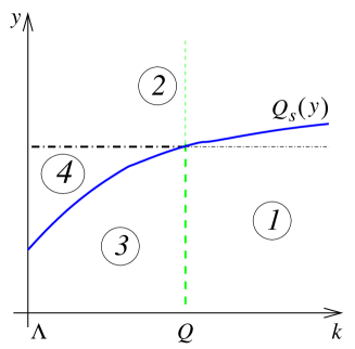
FIG. 6.: Various asymptotic kinematical regions discussed in the text. Solid line is the saturation scale $Q_{s}(y)$. Bold lines are the boundaries of different regions.

There are four interesting asymptotic regions of Eq. (56). They are shown in Fig. 6. In the first and second regions the produced gluon momentum $k$ is the largest external momentum scale of the process. The first region in Fig. 6 corresponds to the cases when $k\gg Q_{s}(y)\gg Q$ and $k\gg Q\gg Q_{s}(y)$, while in the second region $Q_{s}(y)\gg k\gg Q$ and $Q_{s}(y)\gg Q\gg k$. We can find asymptotic behavior of the inclusive cross section by expanding function $\chi(\lambda)$ near its simple pole at $\lambda=0$ and evaluating the Mellin transform in $\lambda$ in the saddle point approximation. This corresponds to the double logarithmic approximation to the evolution equation which means summation of $\alpha^{n}\ln^{n}k\ (Y-y)^{n}\sim 1$ terms. The third and fourth regions in Fig. 6 depict the cases when $Q\gg k\gg Q_{s}(y)$ and $Q\gg Q_{s}(y)\gg k$ correspondingly. In the third and fourth regions asymptotic behavior of the inclusive cross section can be found by repeating this procedure near the simple pole of $\chi(\lambda)$ at $\lambda=1$ which again corresponds to summation of $\alpha^{n}\ln^{n}k\ (Y-y)^{n}\sim 1$ terms. These are two asymptotic double logarithmic regions relevant to the linear evolution before the gluon has been emitted. Generally, after its emission the evolution is nonlinear. So, there is a kinematical domain where the parton density is large (regions 2 and 4 in Fig. 6). In this domain a color dipole evolves into two dipoles, one of which is of the size $1/Q_{s}(y)$. And there is a kinematical domain where the parton density is small (regions 1 and 3) and the evolution is still linear.

Integration over $z$ in Eq. (56) yields a combination of generalized hypergeometric functions which can be expanded near $\lambda=0$ and $\lambda=1$ to give

$$\int_{0}^{\infty}\frac{dz}{z}\,\left(\frac{r}{z}\right)^{2\lambda}z^{2}J_{0}(lz)\left[\frac{2kz}{\lambda}J_{1}(kz)-\frac{k^{2}z^{2}}{2\lambda^{2}}J_{0}(kz)+2J_{0}(kz)\right]=\left\{\begin{array}[]{c}\frac{4(kr)^{2\lambda}}{k^{2}\lambda},\;\lambda\rightarrow 0,\,k\gg l,\\ \\ \\ \frac{4k^{2}(lr)^{2\lambda}}{l^{4}\lambda},\;\lambda\rightarrow 0,\,k\ll l,\\ \\ \\ \frac{(kr)^{2\lambda}}{k^{2}(1-\lambda)},\;\lambda\rightarrow 1,\,k\gg l,\\ \\ \\ \frac{(lr)^{2\lambda}}{l^{2}(1-\lambda)},\;\lambda\rightarrow 1,\,k\ll l.\end{array}\right.$$ (57)

Each of the limits in Eq. (57) corresponds to the appropriate region in Fig. 6. It is now straightforward to evaluate the Mellin transform in the saddle point approximation, which corresponds to the double logarithmic approximation of the scattering amplitude. Using Eq. (57) in Eq. (56) we obtain in the region with $k\gg l$ and $\lambda=0$

$$\frac{d\sigma^{\gamma^{*}A\rightarrow q{\bar{q}}GX}}{d^{2}k\,dy}=\frac{8}{(2\pi)^{3}}\frac{\bar{\alpha}_{s}}{\pi}\frac{\sqrt{\pi}}{\underline{k}^{4}}\int\,d^{2}r\,d\alpha\,\Phi^{\gamma^{*}\rightarrow q{\bar{q}}}(\underline{r},\alpha)\frac{e^{2\sqrt{\bar{\alpha}_{s}(Y-y)\ln(k^{2}r^{2})}}}{\left(\bar{\alpha}_{s}\ln(k^{2}r^{2})(Y-y)\right)^{1/4}}\,\int_{0}^{k}\,dl\,l\,\tilde{N}_{G}(l,y),$$ (58)

We used the well-known expansion $\chi(\lambda)=\lambda^{-1}+\mathcal{O}(\lambda)$. Scattering amplitude $N_{G}(l,y)$ must be normalized to give the correct Fourier transformed initial condition Eq. (53). We have (neglecting logarithmic dependence of $Q_{s}$ on $l$)

$$\tilde{N}_{G}(l,0)=\frac{Q_{0}^{2}}{l^{2}}\int\frac{d\lambda}{2\pi i}\left(\frac{l}{Q_{0}}\right)^{2\lambda}2^{-2\lambda-1}\left(\frac{Q_{0}}{Q_{0s}}\right)^{2\lambda-2}\frac{\Gamma(1-\lambda)}{1-\lambda}=\frac{1}{2}\Gamma\left(0,\frac{l^{2}}{Q_{s}^{2}}\right),$$ (59)

where $\Gamma(0,z)$ is the incomplete gamma function of zeroth order. In the region 1, where $l\gg Q_{s}$, evolution is linear and the scattering amplitude is small. In the linear region

$$N_{G}(l,y)=\frac{Q_{0s}^{2}\pi R^{2}}{2l^{2}}\int\frac{d\nu}{2\pi i}\left(\frac{l}{Q_{0}}\right)^{2\nu}e^{\frac{\bar{\alpha}_{s}}{\nu}y}=\frac{Q_{0s}^{2}\pi R^{2}}{2\pi\,l^{2}}\frac{\sqrt{\pi}\bar{\alpha}_{s}^{1/4}\,y^{1/4}}{\ln^{3/4}(l^{2}/Q_{0}^{2})}e^{2\sqrt{\bar{\alpha}_{s}y\ln(l^{2}/Q_{0}^{2})}},\quad\ln(l/Q_{0})\gg\bar{\alpha}_{s}y,$$ (60)

where we expanded $\chi(\nu)$ near $\nu=0$ and assumed the nucleus to be a cylinder with the cross sectional area $S_{\perp}=\pi R^{2}$. $Q_{0}$ is an initial scale for linear evolution. Eq. (60) gives gluon scattering amplitude in double logarithmic approximation with the expansion parameter $\bar{\alpha}_{s}\,y\ln(l/Q_{0})\sim 1$. Upon substitution of Eq. (60) into Eq. (58) and integration over $l$ one arrives at the asymptotic expression for the inclusive cross section in the region 1

$$\left.\frac{d\sigma^{\gamma^{*}A\rightarrow q{\bar{q}}GX}}{d^{2}k\,dy}\right|_{\mbox{region}\,1}=\frac{\pi R^{2}}{(2\pi)^{4}}\frac{\bar{\alpha}_{s}\,Q_{0s}^{2}}{2\underline{k}^{4}}\int\,d^{2}r\,d\alpha\,\Phi^{\gamma^{*}\rightarrow q{\bar{q}}}(\underline{r},\alpha)\frac{e^{2\sqrt{\bar{\alpha}_{s}(Y-y)\ln(k^{2}r^{2})}+2\sqrt{\bar{\alpha}_{s}y\ln(k^{2}/Q_{0s}^{2})}}}{\bar{\alpha}_{s}^{1/2}\,[y(Y-y)]^{1/4}(\ln k^{2}/Q_{0s}^{2})^{1/4}\ln^{1/4}(k^{2}r^{2})}.$$ (61)

In the region 2 with $l\ll Q_{s}$ saturation sets in and the total scattering amplitude $N(\underline{x},y)$ is close to unity. Thus, using Eq. (29) we conclude that $N_{G}(\underline{x},y)$ is close to unity as well. In the momentum representation this is equivalent to the following asymptotic behavior in the saturation regime [12]

$$\tilde{N}_{G}(l,y)=\ln(Q_{s}(y)/l),\quad l\ll Q_{s}(y).$$ (62)

Using Eq. (62) together with the second line of Eq. (57) in Eq. (58) yields

$$\left.\frac{d\sigma^{\gamma^{*}A\rightarrow q{\bar{q}}GX}}{d^{2}k\,dy}\right|_{\mbox{region}\,2}=\frac{16\pi R^{2}}{(2\pi)^{4}}\sqrt{\pi}\frac{\bar{\alpha}_{s}}{\underline{k}^{2}}\ln\frac{Q_{s}^{2}(y)}{k^{2}}\int\,d^{2}r\,d\alpha\,\Phi^{\gamma^{*}\rightarrow q{\bar{q}}}(\underline{r},\alpha)\frac{e^{2\sqrt{\bar{\alpha}_{s}(Y-y)\ln(k^{2}r^{2})}}}{\left(\bar{\alpha}_{s}\,(Y-y)\ln(k^{2}r^{2})\right)^{1/4}}.$$ (63)

Consider now $\lambda=1$ pole of function $\chi(\lambda)$ in Eq. (56). In the vicinity of this point $\chi(\lambda)=(1-\lambda)^{-1}+\mathcal{O}$$(1-\lambda)$. Substituting the third line of Eq. (57) into Eq. (57) and repeating the above procedure we end up with following asymptotics in the third kinematical region. In the region 3 ($Q\gg k\gg Q_{s}$)

$$\left.\frac{d\sigma^{\gamma^{*}A\rightarrow q{\bar{q}}GX}}{d^{2}k\,dy}\right|_{\mbox{region}\,3}=\frac{\pi R^{2}}{(2\pi)^{4}}\frac{\bar{\alpha}_{s}\,Q_{0s}^{2}}{\underline{k}^{2}}\int d^{2}r\,d\alpha\,\Phi^{\gamma^{*}\rightarrow q{\bar{q}}}(\underline{r},\alpha)\,r^{2}\,\frac{e^{2\sqrt{\bar{\alpha}_{s}(Y-y)\ln(1/k^{2}r^{2})}+2\sqrt{\bar{\alpha}_{s}y\ln(k^{2}/Q_{0s}^{2})}}}{\bar{\alpha}_{s}^{1/2}[y(Y-y)]^{1/4}\left(\ln(k^{2}/Q_{0s}^{2})\ln(1/k^{2}r^{2})\right)^{1/4}}.$$ (64)

Inserting the last line of Eq. (57) into Eq. (56) and using Eq. (62) together with the expression for $N_{G}$ generated by linear evolution gives for the region 4 ($k\ll Q_{s}\ll Q$)

$$\left.\frac{d\sigma^{\gamma^{*}A\rightarrow q{\bar{q}}GX}}{d^{2}k\,dy}\right|_{\mbox{region}\,4}=\frac{4\pi R^{2}}{(2\pi)^{4}}\frac{\bar{\alpha}_{s}\,Q_{s}^{2}(y)}{\underline{k}^{2}}\sqrt{\pi}\int\,d^{2}r\,d\alpha\,\Phi^{\gamma^{*}\rightarrow q{\bar{q}}}(\underline{r},\alpha)\,r^{2}\,\frac{e^{2\sqrt{\bar{\alpha}_{s}\,(Y-y)\ln(1/Q_{s}^{2}(y)r^{2})}}}{\left(\bar{\alpha}_{s}\,(Y-y)\ln(1/Q_{s}^{2}(y)r^{2})\right)^{1/4}},$$ (65)

where the integration over $l$ has been done with logarithmic accuracy.

Note that the spectrum of produced gluons falls off as $\sim k^{-4}$ in region 1, which is a well-known result of the perturbation theory. One factor of $k^{-2}$ arises from the Lipatov’s effective vertex, while another one is given by the perturbative behavior of the scattering amplitude $\nabla^{2}N_{G}$ which scales as $\sim k^{-2}$ at large $k_{\perp}$. When the typical momentum $l$ of the late evolution is less than the saturation scale $Q_{s}(y)$, the anomalous dimension of the gluon structure function is close to unity. Thus the scattering amplitude depends only logarithmically on momentum. As a result, in the region 2 the gluon spectrum softens to $k^{-2}$ behavior. In the region 3 the late evolution is linear like in region 1. However an additional factor of $k^{2}$ stems from different double logarithmic asymptotics at $\lambda=1$. It is remarkable that unlike the regions 1 and 2, the spectrum in region 4 drops in the same manner as in the region 3 despite the fact that the late evolution is nonlinear. This happens because the typical value of $l$ in the rightmost integral in Eq. (58) is $l\sim Q_{s}$. Due to this fact Eq. (65) is enhanced by a factor of $Q_{s}^{2}$ rather than $k^{2}$. Of course, one could not expect that the spectrum will depend on produced gluon’s momentum only logarithmically in the presence of a hard projectile (virtual photon) which wave function has not reached saturation yet.

Derived asymptotic formulae Eq. (61), Eq. (63), Eq. (64) and Eq. (65) make it possible to understand some important features of the spectrum energy dependence. Equating the $y$ derivative of the expression in the exponent of Eq. (61) (or Eq. (64)) to zero one finds the position of the inclusive spectrum maximum $y_{0}$ at some fixed $k$ in the double logarithmic approximation in which the pre-exponential factor is a slowly varying function. It reads

$$y_{0}=Y\frac{1}{1\pm\frac{\ln^{2}(kr)}{\ln^{2}(k/Q_{0s})}}\stackrel{{\scriptstyle k\gg Q,Q_{0s}}}{{\longrightarrow}}\frac{1}{2}Y,$$ (66)

where $+$ and $-$ correspond to the regions 1 and 3. By analogy we find that in the region 2 spectrum is a monotonically decreasing function of $y$ and exhibits no maximum. In the region 4 the spectrum has no maximum in $y$ as well. The following equation defines a surface in the space of parameters where spectrum is constant:

$$\left(4\bar{\alpha}_{s}Y+\ln^{2}\frac{1}{Q_{s}^{2}(0)r^{2}}\right)^{2}=16\bar{\alpha}_{s}Y\ln\frac{1}{Q_{s}^{2}(0)r^{2}}.$$ (67)

Although Eq. (67) is beyond the validity of the double logarithmic approximation employed in this section, it shows the general feature of the spectrum $y$-dependence in region 4. Namely, when $Q\sim Q_{s}$ the spectrum is a step-like function. In Fig. 7 we show a qualitative picture of the energy behavior of the inclusive cross section given by Eq. (36) in different kinematical regions.

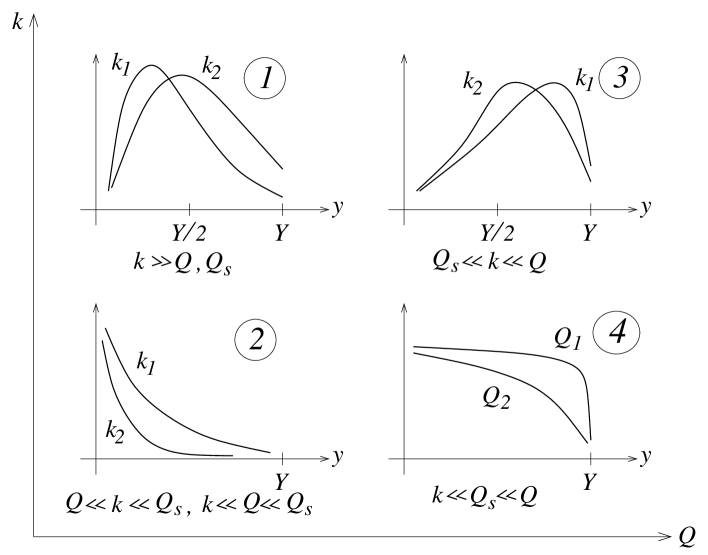
FIG. 7.: Qualitative energy dependence of the inclusive gluon production cross section. All lines are scaled by different numerical factors to underline important features of the spectrum. In all plots we show the curves for two different values of $k$ and/or $Q$ ($k_{1}<k_{2}$, $Q_{1}<Q_{2}$).

Note, that all four plots in Fig. 7 show different qualitative behavior of the inclusive cross section as the rapidity varies. By plotting the experimental data on the energy dependence of the spectrum one can distinguish between different kinematical regions which may be useful for evaluation of the saturation scale. However, we realize that our calculations in the asymptotic regions presented in this Section are approximate and an exact numerical analysis of the cross section in Eq. (45) has to be performed to enable us to describe the data with it.

VI Conclusions

We have constructed an expression for single inclusive gluon production cross section in DIS (Eq. (36)) including multiple pomeron exchanges in the form of nonlinear evolution (Eq. (3)). The cross section may be used to describe (mini)jet production in DIS. For the case of a large target nucleus the resulting production cross section can be written in $k_{T}$–factorized form of Eq. (45). The transverse momentum spectrum given by the cross section of Eq. (36) reproduces the usual perturbative behavior $\sim 1/{\underline{k}}^{4}$ in the large $k_{\perp}$ limit (see Eqs. (61) and (63)). In the small transverse momentum region the spectrum softens to $\sim 1/{\underline{k}}^{2}$ (see Eqs. (64) and (65)). The cross section still exhibits some residual infrared divergence. This is due to the fact that we are scattering a point-like probe (virtual photon) on the target. The target nucleus’ wave function has reached saturation and this is why the $k_{\perp}$ dependence softens in the infrared. However, for the cross section to be infrared safe (up to logarithms), similar to [31], we need the wave functions of both colliding particles to reach saturation. In [31] that was reached for the case of nucleus-nucleus scattering where both nuclear wave functions were in the saturation region. In our case the wave function of the quark-antiquark pair has not reached saturation yet. The onset of saturation in the $\gamma^{*}$ wave function would again be due to multiple pomeron exchanges. Unlike the case of a nucleus with nucleons there is no extra non-perturbative color charges in the original incoming $\gamma^{*}$ wave function to facilitate saturation. All the color charges have to be generated perturbatively. Therefore the multiple pomeron exchanges in the $\gamma^{*}$ wave function would take the form of pomeron loops [8, 39]. Summation of pomeron loops is a separate problem and is beyond the scope of this paper. The effects of pomeron loops can be safely neglected in the energy range considered here.

The result of Eq. (36) could be generalized to the case of proton-nucleus scattering (pA). If one models proton as a dipole made out of diquark and a quark the inclusive gluon production cross section can be obtained by appropriately modifying the linear evolution term (Eq. (24)) and changing the $\gamma^{*}$ wave function into the proton’s wave function. In a more generic case of a proton consisting of $N_{c}$ valence quarks the generalization is probably a bit more involved, though the preceding evolution still remains linear and the gluon production mechanism would not be modified.

We have shown that the evolution in the nuclear wave function (at least in the large-$N_{c}$ limit) can be included via a simple substitution of the Glauber-Mueller amplitude by the dipole-evolved amplitude as presented in Eq. (28). We may therefore try to apply this principle to nucleus-nucleus collisions (AA). In [31] it was argued that the multiplicity of produced gluons in a central nuclear collision is likely to be given by the following formula:

$$\frac{dN^{AA}_{cl}}{d^{2}k\,d^{2}b\,dy}\ =\ \frac{2\,C_{F}}{\alpha_{s}\pi^{2}}\,\left\{-\int\frac{d^{2}z}{(2\pi)^{2}}\,e^{i{\underline{k}}\cdot{\underline{z}}}\,\frac{1}{{\underline{z}}^{2}}\,\left(1-e^{-{\underline{z}}^{2}\,Q_{0s1}^{2}(b)/4}\right)\,\left(1-e^{-{\underline{z}}^{2}\,Q_{0s2}^{2}(b)/4}\right)+\right.$$

$$+\left.\int\frac{d^{2}x\ d^{2}y}{(2\pi)^{3}}\,e^{i{\underline{k}}\cdot({\underline{x}}-{\underline{y}})}\,\frac{{\underline{x}}}{{\underline{x}}^{2}}\cdot\frac{{\underline{y}}}{{\underline{y}}^{2}}\,\left[\frac{1}{{\underline{x}}^{2}\,\ln\frac{1}{|{\underline{x}}|\mu}}\,\left(1-e^{-{\underline{x}}^{2}\,Q_{0s1}^{2}(b)/4}\right)\,\left(1-e^{-{\underline{x}}^{2}\,Q_{0s2}^{2}(b)/4}\right)+\right.\right.$$

$$+\left.\left.\frac{1}{{\underline{y}}^{2}\,\ln\frac{1}{|{\underline{y}}|\mu}}\,\left(1-e^{-{\underline{y}}^{2}\,Q_{0s1}^{2}(b)/4}\right)\,\left(1-e^{-{\underline{y}}^{2}\,Q_{0s2}^{2}(b)/4}\right)\right]\right\}.$$ (68)

$Q_{0s1}^{2}(b)$ and $Q_{0s2}^{2}(b)$ are the saturation scales in each of nuclei taken at the same impact parameter since the collisions considered are central. Inspired by the success of the substitution (28) in incorporating the quantum evolution corrections in DIS we may conjecture the following ansatz for the multiplicity distribution of the produced gluons in AA including nonlinear evolution in the wave functions of both nuclei

$$\frac{dN^{AA}}{d^{2}k\,d^{2}b\,dy}\ =\ \frac{2\,C_{F}}{\alpha_{s}\pi^{2}}\,\left\{-\int\frac{d^{2}z}{(2\pi)^{2}}\,e^{i{\underline{k}}\cdot{\underline{z}}}\,\frac{1}{{\underline{z}}^{2}}\,N_{G1}({\underline{z}},{\underline{b}},y)\,N_{G2}({\underline{z}},{\underline{b}},Y-y)+\right.$$

$$+\left.\int\frac{d^{2}x\ d^{2}y}{(2\pi)^{3}}\,e^{i{\underline{k}}\cdot({\underline{x}}-{\underline{y}})}\,\frac{{\underline{x}}}{{\underline{x}}^{2}}\cdot\frac{{\underline{y}}}{{\underline{y}}^{2}}\,\left[\frac{1}{{\underline{x}}^{2}\,\ln\frac{1}{|{\underline{x}}|\mu}}\,N_{G1}({\underline{x}},{\underline{b}},y)\,N_{G2}({\underline{x}},{\underline{b}},Y-y)+\right.\right.$$

$$+\left.\left.\frac{1}{{\underline{y}}^{2}\,\ln\frac{1}{|{\underline{y}}|\mu}}\,\,N_{G1}({\underline{y}},{\underline{b}},y)\,N_{G2}({\underline{y}},{\underline{b}},Y-y)\,\right]\right\},$$ (69)

where $Y$ is the total rapidity interval and $N_{G1}$ and $N_{G2}$ are adjoint dipole forward scattering amplitudes in the first and second nucleus correspondingly. At the moment we can not prove Eq. (69) and leave it as an ansatz inspired by the properties of the inclusive cross sections in the saturation region studied above. We may argue that the final state gluon mergers which are not included in Eq. (68) are not likely to give logarithms of energy and therefore should not contribute to the quantum evolution. They might be neglected compared to the evolution effects included in Eq. (69). Eq. (69), together with Eq. (3), may be used to describe the emerging RHIC data similar to how it was done in [41].

REFERENCES

- [1] L. V. Gribov, E. M. Levin, and M. G. Ryskin, Phys. Rep. 100, 1 (1983); A.H. Mueller, J.-W. Qiu, Nucl. Phys. B268, 427 (1986).
- [2] E.M. Levin and M.G Ryskin, Nucl. Phys. B304, 805 (1988); Sov. J. Nucl. Phys. 45, 150 (1987); 41, 300 (1985).
- [3] A.H. Mueller, Nucl. Phys. B335, 115 (1990).
- [4] L. McLerran and R. Venugopalan, Phys. Rev. D 49, 2233 (1994); 49, 3352 (1994); 50, 2225 (1994).
- [5] Yu.V. Kovchegov, Phys. Rev. D 54, 5463 (1996); 55, 5445 (1997).
- [6] J. Jalilian-Marian, A. Kovner, L. McLerran, and H. Weigert, Phys. Rev. D 55,5414 (1997).
- [7] Yu. V. Kovchegov, Phys. Rev. D 60, 034008 (1999); D 61, 074018 (2000).
- [8] A.H. Mueller, Nucl. Phys. B415, 373 (1994); A.H. Mueller and B. Patel, Nucl. Phys. B425, 471 (1994); A.H. Mueller, Nucl. Phys. B437, 107 (1995).
- [9] Z. Chen, A.H. Mueller, Nucl. Phys. B451, 579 (1995).
- [10] I. I. Balitsky, Report No. hep-ph/9706411; Nucl. Phys. B463, 99 (1996); Phys. Rev. D 60, 014020 (1999).
- [11] J. Jalilian-Marian, A. Kovner, A. Leonidov, and H. Weigert, Nucl. Phys. B 504, 415 (1997); Phys. Rev. D 59 014014 (1999); Phys. Rev. D59, 034007 (1999); J. Jalilian-Marian, A. Kovner, and H. Weigert, Phys. Rev. D 59 014015 (1999); A. Kovner, J. G. Milhano, H. Weigert, Phys. Rev. D 62, 114005 (2000); H. Weigert, hep-ph/0004044; E. Iancu, A. Leonidov, L. McLerran, Nucl. Phys. A692, 583 (2001); Phys. Lett. B510, 133 (2001); E. Iancu and L. McLerran, Phys. Lett. B510, 145 (2001); E. Ferreiro, E. Iancu, A. Leonidov, L. McLerran, hep-ph/0109115.
- [12] E. Levin and K. Tuchin, Nucl. Phys. B573, 833 (2000); Nucl. Phys. A691, 779 (2001); Nucl. Phys. A693, 787 (2001).
- [13] M. A. Braun, Eur. Phys. J. C 16, 337 (2000); hep-ph/0010041; hep-ph/0101070.
- [14] A.L.Ayala, M.B.Gay Ducati, E.M.Levin, Nucl. Phys. B493, 305 (1997); Nucl. Phys. B511, 355 (1998); Eur. Phys. J. C8, 115 (1999).
- [15] C.S. Lam, G. Mahlon, Phys. Rev. D61, 014005 (2000); Phys. Rev. D62, 114023 (2000); Phys. Rev. D64, 016004 (2001).
- [16] E. Levin and M. Lublinsky, hep-ph/0104108; M. Lublinsky,E. Gotsman, E. Levin and U. Maor, hep-ph/0102321.
- [17] K. Golec-Biernat, L. Motyka, A.M. Stasto, hep-ph/0110325.
- [18] A. H. Mueller, Nucl. Phys. B572, 227 (2000); Nucl. Phys. B558, 285 (1999); hep-ph/0111244.
- [19] Yu. V. Kovchegov, A.H. Mueller, Nucl. Phys. B529, 451 (1998).
- [20] E.A. Kuraev, L.N. Lipatov and V.S. Fadin, Sov. Phys. JETP 45, 199 (1977); Ya.Ya. Balitsky and L.N. Lipatov, Sov. J. Nucl. Phys. 28, 22 (1978).
- [21] Yu. V. Kovchegov, Phys. Rev. D 64, 114016 (2001).
- [22] I.I. Balitsky, A.V. Belitsky, hep-ph/0110158.
- [23] A. Hebecker, Nucl.Phys. B505, 349 (1997); W. Buchmüller, M. F. McDermott, and A. Hebecker, Phys. Lett. B 410, 304 (1997); W. Buchmüller, T. Gehrmann, and A. Hebecker, Nucl.Phys. B537, 477 (1999); Yu. V. Kovchegov and L. McLerran, Phys. Rev. D 60, 054025 (1999); Erratum-ibid. D 62, 019901 (2000).
- [24] Yu. V. Kovchegov, E. Levin, Nucl. Phys. B577, 221 (2000).
- [25] A. Kovner, L. McLerran, and H. Weigert, Phys. Rev. D 52, 6231 (1995); 52, 3809 (1995); M. Gyulassy, L. McLerran, Phys. Rev. C 56, 2219 (1997); Yu.V. Kovchegov, D. H. Rischke, Phys. Rev. C 56, 1084 (1997); X. Guo, Phys. Rev, D 59, 094017 (1999).
- [26] J.F. Gunion and G. Bertsch, Phys. Rev. D 25, 746 (1982).
- [27] B. Z. Kopeliovich, A. V. Tarasov, A. Schafer, Phys. Rev. C 59, 1609 (1999); B. Z. Kopeliovich, A. Schafer, A. V. Tarasov, Phys. Rev. D 62, 054022 (2000); B. Kopeliovich, A. Tarasov, J. Hufner, hep-ph/0104256.
- [28] A. Dumitru, L. McLerran, hep-ph/0105268; A. Dumitru, J. Jalilian-Marian, hep-ph/0111357.
- [29] A. Kovner, U. A. Wiedemann, Phys. Rev. D 64, 114002 (2001).
- [30] A. Krasnitz, R. Venugopalan, Report No. hep-ph/0007108; Phys. Rev. Lett. 84, 4309 (2000); Nucl. Phys. B557, 237 (1999); A. Krasnitz, Y. Nara, R. Venugopalan, Phys. Rev. Lett. 87, 192302 (2001).
- [31] Yu. V. Kovchegov, Nucl. Phys. A692, 557 (2001); Nucl. Phys. A698, 619c (2002).
- [32] N. Armesto, M.A. Braun, hep-ph/0107114.
- [33] L. V. Gribov, E. M. Levin, and M. G. Ryskin, Phys. Lett. B100, 173 (1981).
- [34] M. A. Braun, Phys. Lett. B483, 105 (2000).
- [35] V. A. Abramovsky, V. N. Gribov, O. V. Kancheli, Sov. J. Nucl. Phys. 18, 308 (1974).
- [36] E. M. Levin, hep-ph/9710546.
- [37] S. J. Brodsky, B.-Q. Ma, Phys. Lett. B381, 317 (1996); S. J. Brodsky, P. Hoyer, C. Peterson, N. Sakai, Phys. Lett. B93, 451 (1980); S. J. Brodsky, C. Peterson, N. Sakai, Phys. Rev. D 23, 2745 (1981).
- [38] G. P. Lepage, S. J. Brodsky, Phys. Rev. D 22, 2157 (1980); S. J. Brodsky, R. Roskies, R. Suaya, Phys. Rev. D 8, 4574 (1973); P. P. Srivastava, S. J. Brodsky, Phys. Rev. D 64, 045006 (2001).
- [39] H. Navelet, R. Peschanski, C. Royon, S. Wallon, Phys. Lett. B385, 357 (1996); H. Navelet, R. Peschanski, Phys. Rev. Lett. 82, 1370 (1999); A. Bialas, H. Navelet, R. Peschanski, Nucl. Phys. B593, 438 (2001).
- [40] R. Baier, Yuri L. Dokshitzer, A.H. Mueller, S. Peigne, D. Schiff, Nucl. Phys. B483, 291 (1997).
- [41] D. Kharzeev, E. Levin, nucl-th/0108006; D. Kharzeev, E. Levin, M. Nardi, hep-ph/0111315.