Baryon magnetic moments in the effective quark Lagrangian approach

Abstract

An effective quark Lagrangian is derived from first principles through bilocal gluon field correlators. It is used to write down equations for baryons, containing both perturbative and nonperturbative fields. As a result one obtains magnetic moments of octet and decuplet baryons without introduction of constituent quark masses and using only string tension as an input. Magnetic moments come out on average in reasonable agreement with experiment, except for nucleons and $\Sigma^{-}$. The predictions for the proton and neutron are shown to be in close agreement with the empirical values once we choose the string tension such to yield the proper nucleon mass. Pionic corrections to the nucleon magnetic moments have been estimated. In particular, the total result of the two-body current contributions are found to be small. Inclusion of the anomalous magnetic moment contributions from pion and kaon loops leads to an improvement of the predictions.

I Introduction

The QCD dynamics of $q\bar{q}$ and $3q$ systems is governed by two basic phenomena: confinement and chiral symmetry breaking (CSB), which should be treated in a fully relativistically covariant way. Confinement is usually introduced for static quarks via the area law of the Wilson loop [1] or equivalently through the field correlators in the Field Correlator Method (FCM) [2, 3].

For spinless quarks, or neglecting spin–dependent mass corrections, one can envisage a self–consistent method which treats confinement as the area law also for light quarks in a relativistically covariant way. Such method was introduced originally in [4] for mesons, in [5] for baryons, and in [6] for heavy–light mesons, and later on in [7] the method was generalized taking into account the dynamical degrees of freedom of the QCD string, which naturally appears due to the area law.

As a result Regge trajectories have been found in [7] with the correct string slope $(2\pi\sigma)^{-1}$. It was realized later on, that the method used in [4]-[7] can be more generally developed in the framework of the so-called einbein formalism, see [8]-[10]. Spin corrections have been considered in [11] for heavy mesons and in [6] for heavy–light ones. In the general case of light quarks spin-dependent correlations have been introduced in [12], and for gluons in [13]. For a general review with explicit formulae see [14]. Baryon Regge trajectories have been found in [5]. In all cases the basic formalism is the FCM and the Feynman–Schwinger (or world-line) path integral representation [3, 15, 16] which is well suited for relativistic quarks when spin is considered as a perturbation.

The main difficulty which was always present in the method, was the perturbative treatment of spin degrees of freedom (which is incorrect, e.g., for the pion) and absence of spontaneous CSB effects in general [17]. Recently a new type of formalism was suggested to treat simultaneously confinement and CSB and a nonlinear equation was derived for a light quark in the field of heavy antiquark [18]. This equation derived directly from QCD Lagrangian was found to produce linear confinement and CSB for the light quark and the explicit form of the effective quark mass operator $M(x,y)$ was defined obeying both these properties.

The eigenvalues and eigenfunctions of the nonlocal and nonlinear equations have been determined and a nonzero condensate was computed in [19], confirming that CSB is really present in the equations. In an additional study [20] it was demonstrated that magnetic field correlators do not contribute to the large distance confinement, however strongly modify the confinement for lowest levels and heavy-light masses corrected in this way are favourably compared in [20] to the experiment and results of other calculations.

Moreover, it was shown in [21] that lattice data strongly support the dominance of the Gaussian (bilocal) correlator, estimating the correction due to higher correlators to 1-2%. Since the method of [18] is quite general and allows to treat also multiquark systems, it can be applied to the $q\bar{q}$ and $3q$ systems, to find dynamical equations for them, which contain confinement and CSB [22]. To make these equations tractable, one systematically exploits the large $N_{c}$ limit, and mostly confine ourselves to the simplest field correlators – the so–called Gaussian approximation; it was in particular shown in [18] that the sum over all correlators does not change the qualitative results. However, the kernel of equations becomes much more complicated.

In the present paper we study the baryon magnetic moments based on the derived effective Lagrangian without constituent quark masses. The paper is organized as follows. In Section 2 the general effective quark Lagrangian from the standard QCD Lagrangian is obtained by integrating out gluonic degrees of freedom, and the nonlinear equation for the single quark propagator $S$ (attached to the string in a gauge–invariant way) is derived, following the procedure in [22]. Section 3 is devoted to the baryon Green’s function, which can be expressed in the lowest order of our approximation scheme (neglecting gluon and pion exchanges) in terms of 3 independent quark Green’s function, resulting in a Hamiltonian as a sum of three quark terms. In section 4 the next order approximation is written down when perturbative gluon exchanges are taken into account, including the nonperturbative interaction between quarks violating the factorized form of the zeroth order approximation. The next section is devoted to the calculation of magnetic moments of baryons both in octet and decuplet representations of SU(3) flavour group. In section 6 we discuss the corrections to magnetic moments due to pion exchange contributions.

II Effective quark Lagrangian

As was discussed in the previous section, one can obtain an effective quark Lagrangian by averaging over background gluonic fields. We shall repeat this procedure following [18] now paying special attention to the dependence on the contour in the definition of contour gauge, and introducing the operation of averaging over contour manifold. The QCD partition function for quarks and gluons can be written as

$$Z=\int DAD\psi D\psi^{+}{\rm exp}[L_{0}+L_{1}+L_{{\rm int}}],$$ (1)

where we are using Euclidean metric and define

$$L_{0}=-\frac{1}{4}\int d^{4}x(F^{a}_{\mu\nu})^{2},$$ (2)

$$L_{1}=-i\int~{}^{f}\psi^{+}(x)(\hat{\partial}+m_{f})~{}^{f}\psi(x)d^{4}x,$$ (3)

$$L_{\rm int}=\int~{}^{f}\psi^{+}(x)g\hat{A}(x)~{}^{f}\psi(x)d^{4}x.$$ (4)

Here and in what follows $~{}^{f}\psi_{a\alpha}$ denotes quark operator with flavour $f$, color $a$ and bispinor index $\alpha$.

To express $A_{\mu}(x)$ through $F_{\mu\nu}$ one can use the generalized Fock–Schwinger gauge [23] with the contour $C(x)$ from the point $x$ to $x_{0}$, which can also lie at infinity,

$$A_{\mu}(x)=\int_{c}F_{\lambda\beta}(z)\frac{\partial z_{\beta}(s,x)}{\partial x_{\mu}}\frac{\partial z_{\lambda}}{\partial s}ds.$$ (5)

Now one can integrate out the gluonic field $A_{\mu}(x)$, and introduce an arbitrary integration over the set of contours $C(x)$ with the weight $D_{\kappa}(C)$, since $Z$ is gauge invariant it does not depend on the contour $C(x)$. One obtains

$$Z=\int D\kappa(C)D\psi D\psi^{+}{\rm exp}\{L_{1}+L_{\rm eff}\},$$ (6)

where the effective quark Lagrangian $L_{\rm eff}$ is defined as

$${\rm exp}L_{\rm eff}=\langle{\rm exp}\int~{}^{f}\psi^{+}\hat{A}~{}^{f}\psi d^{4}x\rangle_{A}.$$ (7)

Using the cluster expansion, $L_{\rm eff}$ can be written as an infinite sum containing averages $\langle(\hat{A})^{k}\rangle_{A}$. At this point one can exploit the Gaussian approximation, neglecting all correlators $\langle(\hat{A})^{k}\rangle$ of degree higher than $k=2$. Numerical accuracy of this approximation was discussed and tested in [21]. One expects that for static quarks corrections to Gaussian approximation amount to less than 2-3%.

The resulting effective Lagrangian is quartic in $\psi$,

$$L^{(4)}_{\rm eff}=\frac{1}{2N_{c}}\int d^{4}xd^{4}y^{f}\psi^{+}_{a\alpha}(x)~{}^{f}\psi_{b\beta}(x)~{}^{g}\psi^{+}_{b\gamma}(y)~{}^{g}\psi_{a\delta}(y)J_{\alpha\beta;\gamma\delta}(x,y)+O(\psi^{6}),$$ (8)

$$J_{\alpha\beta,\gamma\delta}(x,y)=(\gamma_{\mu})_{\alpha\beta}(\gamma_{\nu})_{\gamma\delta}J_{\mu\nu}(x,y)$$ (9)

and $J_{\mu\nu}$ is expressed as

$$J_{\mu\nu}(x,y)=g^{2}\int^{x}_{C}\frac{\partial u_{\omega}}{\partial x_{\mu}}du_{\varepsilon}\int^{y}_{C}\frac{\partial u_{\omega^{\prime}}}{\partial y_{\nu}}du_{\varepsilon^{\prime}}\frac{tr}{N_{c}}\langle F_{\varepsilon\omega}(u)F_{\varepsilon^{\prime}\omega^{\prime}}(v)\rangle.$$ (10)

$L_{\rm eff}$, Eq. (8), is written in the contour gauge [23]. It can be identically rewritten in the gauge–invariant form if one substitutes parallel transporters $\Phi(x,x_{0}),\Phi(y,x_{0})$ (identically equal to unity in this gauge) into Eqs. (8) and (10), multiplying each $\psi(x)$ and $\psi(y)$ respectively and replacing $F(u)$ in Eq. (10) by $\Phi(x,u)F(u)\Phi(u,x_{0})$ and similarly for $F(v)$.

After that $L_{\rm eff}$ becomes gauge–invariant, but in general contour–dependent, if one keeps only the quartic term (8), and neglects all higher terms. A similar problem occurs in the cluster expansion of Wilson loop, when one keeps only lowest correlators, leading to the (erroneous) surface dependence of the result. The situation here is the same as with a sum of QCD perturbation series, which depends on the normalization mass $\mu$ for any finite number of terms in the series. This unphysical dependence is usually treated by fixing $\mu$ at some physically reasonable value $\mu_{0}$ (of the order of the inverse size of the system).

The integration over contours $D\kappa(C)$ in (6) resolves this difficulty in a similar way. Namely, the partition function $Z$ formally does not depend on contours (since it is integrated over a set of contours) but depends on the weight $D\kappa(C)$. We choose this weight in such a way, that the contours would generate the string of minimal length between $q$ and $\bar{q}$. Thus the physical choice of the contour corresponds to the minimization of the meson (baryon) mass over the class of strings, in the same way as the choice of $\mu=\mu_{0}$ corresponds to the minimization of the dropped higher perturbative terms. As a practical outcome, we shall keep the integral $D\kappa(C)$ till the end and finally use it to minimize the string between the quarks.

Till this point we have made only one approximation –neglected all field correlators except the Gaussian one. Recent lattice calculations (see Refs. [24, 25]) estimate the accuracy of this approximation at the level of few percents. Now one must use another approximation, i.e. assume a large $N_{c}$ expansion and keep the lowest term. As was shown in [18] this enables one to replace in (8) the colorless product $~{}^{f}\psi_{b}(x)~{}^{g}\psi_{b}^{+}(y)=tr(~{}^{f}\psi(x)\Phi(x,x_{0})\Phi(x_{0},y)~{}^{g}\psi^{+}(y))$ by the quark Green’s function

$$~{}^{f}\psi_{b\beta}(x)~{}^{g}\psi^{+}_{b\gamma}(y)\to\delta_{fg}N_{c}S_{\beta\gamma}(x,y).$$ (11)

$L^{(4)}_{\rm eff}$ assumes the form

$$L^{(4)}_{\rm eff}=-i\int d^{4}xd^{4}y~{}^{f}\psi^{+}_{a\alpha}(x)~{}^{f}M_{\alpha\delta}(x,y)~{}^{f}\psi_{a\delta}(y),$$ (12)

where the quark mass operator is

$$~{}^{f}M_{\alpha\delta}(x,y)=-J_{\mu\nu}(x,y)(\gamma_{\mu}~{}^{f}S(x,y)\gamma_{\nu})_{\alpha\delta}.$$ (13)

From (12) it is evident that $~{}^{f}S$ satisfies

$$(-i\hat{\partial}_{x}-im_{f})~{}^{f}S(x,y)-i\int~{}^{f}M(x,z)d^{4}z~{}^{f}S(z,y)=\delta^{(4)}(x-y).$$ (14)

Eqs. (13)-(14) have been first derived in [18]. From (6) and (12) one should expect that at large $N_{c}$ the $q\bar{q}$ and $3q$ dynamics is expressed through the quark mass operator (13), which should contain both confinement and CSB. Indeed, the analysis performed in Refs. [18]-[20] reveals that confinement is present in the long–distance form of $M(x,y)$, when both distances $|\mbox{\boldmath${\rm x}$}|,|\mbox{\boldmath${\rm y}$}|$ of light quark from heavy antiquark (placed at $\mbox{\boldmath${\rm x}$}=0$) are large.

We shall now make several simplifying assumptions, to clarify the structure of $M(x,y)$. First of all we take the class of contours $C$ going from any point $x=(x_{4},\mbox{\boldmath${\rm x}$})$ to the point $(x_{4},0)$ and then to $(-\infty)$ along the $x_{4}$ axis. For this class the corresponding gauge was studied in [26]. Secondly, we take the dominant part of $J_{\mu\nu}$ in (13), namely $J_{44}$, which is proportional to the correlator of color–electric fields. This yields a linear confining interaction, while the other components $J_{ik},J_{i4},J_{4i},i=1,2,3$ have been neglected, containing magnetic fields and yielding momentum dependent corrections. (It is easy to take into account these contributions in a more detailed analysis).

The correlator $\langle FF\rangle$ in (10) can be expressed through the scalar correlator $D(x),$ defined as [2],

$$\frac{trg^{2}}{N_{c}}\langle F_{\alpha\beta}(u)\Phi(u,v)F_{\gamma\delta}(v)\Phi(v,u)\rangle=D(u-v)(\delta_{\alpha\gamma}\delta_{\beta\delta}-\delta_{\alpha\delta}\delta_{\beta\gamma})+O(D_{1}),$$ (15)

where the correlator $D_{1}$, not contributing to confinement, is neglected. As a result one has for $M$ [19, 20]

$$~{}^{f}M_{C_{x_{4}}}(x,y)=~{}^{f}M^{(0)}I+~{}^{f}M^{(i)}\hat{\sigma}_{i}+~{}^{f}M^{(4)}\gamma_{4}+~{}^{f}M^{(i)}_{\gamma}\gamma_{i}.$$ (16)

Here we have defined

$$\hat{\sigma}_{i}=\left(\begin{array}[]{ll}\sigma_{i}&0\\ 0&\sigma_{i}\end{array}\right).$$ (17)

The dominant part of $M$, $~{}^{f}M^{(0)}$ is linearly growing at large $|\mbox{\boldmath${\rm x}$}|,|\mbox{\boldmath${\rm y}$}|$ and in the most simple case of Gaussian form of $D(x)$, can be written as

$$~{}^{f}M^{(0)}(x,y)=\frac{1}{2T_{g}\sqrt{\pi}}e^{-\frac{(x_{4}-y_{4})^{2}}{4T_{g}^{2}}}\sigma|\frac{\mbox{\boldmath${\rm x}$}+\mbox{\boldmath${\rm y}$}}{2}|\tilde{\delta}^{(3)}(\mbox{\boldmath${\rm x}$}-\mbox{\boldmath${\rm y}$})$$ (18)

where $T_{g}$ is the gluon correlation length, and $\tilde{\delta}$ is a smeared $\delta$–function, which can be represented as [19, 20]

$$\tilde{\delta}^{(3)}(\mbox{\boldmath${\rm x}$}-\mbox{\boldmath${\rm y}$})\approx exp(-\frac{|\mbox{\boldmath${\rm x}$}-\mbox{\boldmath${\rm y}$}|^{2}}{b^{2}})(\frac{1}{b\sqrt{\pi}})^{3},~{}~{}b\sim 2T_{g}.$$ (19)

Here again $T_{g}$ is the gluon correlation length, which enters $D(u)$ as $D(u)=D(0){\rm exp}(-\frac{u^{2}}{4T_{g}^{2}})$. We are now in the position to derive the $q\bar{q}$, $3q$ Green’s function, which will be done in the next section.

III Equations for the baryon Green’s function

Equations for the $3q$ system can be written in the same way as for the $q\bar{q}$ system. We again shall assume the large $N_{c}$ limit in the sense, that $1/N_{c}$ corrections from $q\bar{q}$ pairs to the quark Green’s function and the effective mass can be neglected. We now write down the explicit expressions for $N_{c}=3$.

The initial and final field operators are

$$\Psi_{in}(x,y,z)=e_{abc}\Gamma^{\alpha\beta\gamma}\psi_{a\alpha}(x,C(x))\psi_{b\beta}(y,C(y))\psi_{c\gamma}(z,C(z))$$ (20)

with the notations: $a,b,c,$ are color indices, $\alpha,\beta,\gamma$ are Lorentz bispinor indices and transported quark operators are

$$\psi_{a\alpha}(x,C(x))=(\Phi_{C}(x,\bar{x})\psi_{\alpha}(\bar{x}))_{a}.$$ (21)

The contour $C(x)$ in $\Phi_{C}$ can be arbitrary , but it is convenient to choose it in the same class of contours that is used in $D\kappa(C)$ and in the generalized Fock–Schwinger gauge [23]. $\Gamma^{\alpha\beta\gamma}$ is the Lorentz spinor tensor securing proper baryon quantum numbers. One can also choose other operators, but it does not influence the resulting equations. In Eq. (20) we have omitted flavour indices in $\Gamma$ and $\psi(x,C)$, to be easily restored in final expressions.

Using now the effective Lagrangian (12) valid at large $N_{c}$, we obtain for the $3q$ Green’s function.

$$G^{(3q)}(x,y,z|x^{\prime},y^{\prime},z^{\prime})=$$

$$\frac{1}{N}\int D\kappa(C)D\psi D\psi^{+}\Psi_{\rm fin}(x^{\prime},y^{\prime},z^{\prime})\Psi^{+}_{\rm in}(x,y,z){\rm exp}(L_{1}+L_{\rm eff}).$$ (22)

Integrating out quark degrees of freedom and neglecting the determinant at large $N_{c}$, one has

$$G^{(3q)}=\int D\kappa(C)(e\Gamma)(e^{\prime}\Gamma^{\prime})\{S(x,x^{\prime})S(y,y^{\prime})S(z,z^{\prime})+{\rm perm}\},$$ (23)

where for simplicity color and bispinor indices are suppressed together with parallel transporters in initial and final states.

One can also define unprojected (without $\Gamma,\Gamma^{\prime})$ $3q$ Green’s function $G^{(3q)}_{\rm un}$ with 3 initial and 3 final bispinor indices instead of projected by $\Gamma,\Gamma^{\prime}$ quantum numbers of baryon. Assuming that minimization over contours $D\kappa(C)$ reduces to the single choice of the contours (the single string junction trajectory minimizing the mass of baryon), one can write equation for $G_{\rm un}^{(3q)}$:

$$(-i\hat{\partial}_{x}-im_{1}-i\hat{M}_{1})(-i\hat{\partial}_{y}-im_{2}-i\hat{M}_{2})(-i\hat{\partial}_{z}-im_{3}-i\hat{M}_{3})G_{\rm un}^{(3q)}=$$

$$\delta^{(4)}(x-x^{\prime})\delta^{(4)}(y-y^{\prime})\delta^{(4)}(z-z^{\prime})$$ (24)

with e.g. $\hat{M}_{1}G\equiv\int M(x,u)G(u,x^{\prime})d^{4}u$. One can simplify the form (23) for $G^{(3q)}$ taking into account that $M(x,x^{\prime})$ actually does not depend on $\frac{x_{4}+x^{\prime}_{4}}{2}$. Hence the interaction kernel of $G^{(3q)}$ does not depend on relative energies, as in [27]. Similarly to [27, 28] one can introduce Fourier transform of $G^{(3q)}$ in time components and take into account energy conservation $E=E_{1}+E_{2}+E_{3}$. One obtains

$$G^{(3q)}(E,E_{2},E_{3})\simeq\int D\kappa(C)(e\Gamma)(e^{\prime}\Gamma^{\prime})$$

$$\times\frac{1}{(E-E_{2}-E_{3}-H_{1})(E_{2}-H_{2})(E_{3}-H_{3})},$$ (25)

where we have used the notation

$$H_{i}=m_{i}\beta^{(i)}+\mbox{\boldmath${\rm p}$}^{(i)}\mbox{\boldmath${\rm\alpha}$}^{(i)}+\beta^{(i)}M(\mbox{\boldmath${\rm r}$}^{(i)}-\mbox{\boldmath${\rm r}$}^{(0)}).$$ (26)

Moreover, we have taken in $M(x,x^{\prime})$ the limit of small $T_{g}$ and the set of contours in $D\kappa(C)$ passing from the point $\mbox{\boldmath${\rm r}$}^{(i)}$ to some (arbitrary) point $\mbox{\boldmath${\rm r}$}^{(0)}$. As in [27] one can now integrate over $E_{2},E_{3}$ to obtain finally

$$G^{(3q)}(E,\mbox{\boldmath${\rm r}$}_{i},\mbox{\boldmath${\rm r}$}^{\prime}_{i})\simeq\int D\kappa(C)(e\Gamma)(e^{\prime}\Gamma^{\prime})\frac{1}{(E-H_{1}-H_{2}-H_{3})}.$$ (27)

From (27) one obtains equation for the $3q$ wave function similar to that of $q\bar{q}$ system,

$$(H_{1}+H_{2}+H_{3}-E)\psi(\mbox{\boldmath${\rm r}$}_{1},\mbox{\boldmath${\rm r}$}_{2},\mbox{\boldmath${\rm r}$}_{3})=0,$$ (28)

where $\mbox{\boldmath${\rm r}$}^{(0)}$ is to be taken at the Torricelli point. In the nonrelativistic approximation $m_{i}\gg\sqrt{\sigma}$ one has

$$\sum^{3}_{i=1}\left[\frac{(\mbox{\boldmath${\rm p}$}^{(i)})^{2}}{2m_{i}}+\sigma|\mbox{\boldmath${\rm r}$}^{(i)}-\mbox{\boldmath${\rm r}$}^{(0)}|\right]\Psi=\varepsilon\Psi,~{}~{}\varepsilon=E-\sum m_{i}$$ (29)

IV Perturbative corrections to factorized solutions

The effective Lagrangian (8) and the effective mass operator $M(x,y)$, Eq. (13), do not take into account the perturbative interaction between the quarks in the baryon. To this end we separate the gluonic field $A_{\mu}$ into a background $B_{\mu}$ and perturbative parts, $A_{\mu}=B_{\mu}+a_{\mu}$ and use the ’t Hooft identity to integrate in the partition function independently over both parts of $A_{\mu}$ as was done in [30].

We shall use the following representation of gauge transformations

$$B_{\mu}\to U^{+}(B_{\mu}+\frac{i}{g}\partial_{\mu})U,~{}~{}~{}a_{\mu}\to U^{+}a_{\mu}U$$ (30)

and keep for $a_{\mu}$ the background gauge condition [29],[30]

$$D_{\mu}(B)a_{\mu}=0,~{}~{}~{}D_{\mu}(B)=\partial_{\mu}-igB_{\mu}$$ (31)

As a result of the perturbative gluon exchange between different quarks in the baryon there will appear an additional vertex in the effective Lagrangian [19]

$$\Delta L=g^{2}\int^{f}\psi^{+}(x)\gamma_{\mu}^{f}\psi(x)\int^{g}\psi^{+}(y)\gamma_{\nu}^{g}\psi(y)\langle a_{\mu}(x)a_{\nu}(y)\rangle dxdy.$$ (32)

In what follows we shall be interested only in the color Coulomb interaction which results from (32) assuming the simplest form of gluon propagator and neglecting at first for simplicity the influence of the background field on it, namely

$$\int\langle a_{\mu}(x)a_{\nu}(y)\rangle d(x_{4}-y_{4})=\frac{\delta_{\mu\nu}C_{2}}{4\pi^{2}}\int\frac{d(x_{4}-y_{4})}{(\bar{x}-\bar{y})^{2}+(x_{4}-y_{4})^{2}}=\frac{\delta_{\mu\nu}C_{2}}{4\pi|\mbox{\boldmath${\rm x}$}-\mbox{\boldmath${\rm y}$}|}.$$ (33)

Now taking the background into account, one arrives at the picture of the gluon $a_{\mu}$ propagating inside the film – the world sheet of the string, created by the background between three quark worldlines and the string junction, as is shown in Fig. 1. Depending on the choice of $\mbox{\boldmath${\rm r}$}^{(0)}$ we will get in general an effective interaction of a 2-body or 3-body nature. Due to the presence of the QCD background the strength of the resulting Coulomb interaction is expected to be different from the perturbative OGE contribution and as a result different from the interaction used for example in the Breit equation [31].

Due to its attractive nature the color Coulomb contribution leads to smaller baryon masses and giving rise to composite systems with a smaller radius. As a result the magnetic moments become smaller. In the remaining part of the paper we neglect the effect from the Coulomb interaction. To study this a more involved analysis is needed, where also the hyperfine interaction has to be included.

FIG. 1.: A schematic view of the gluon propagating inside the world sheet of the string.

V Baryon magnetic moments without quark constituent masses

Since the calculation of magnetic moments as well as baryon masses does not involve large momentum transfer, one can use for that purpose the Hamiltonian equation (28). According to the results of section 4, $H_{i}$ can be represented as

$$H_{i}=m_{i}\beta^{(i)}+\mbox{\boldmath${\rm p}$}^{(i)}\mbox{\boldmath${\rm\alpha}$}^{(i)}+\beta^{(i)}M^{(i)}(\mbox{\boldmath${\rm r}$}^{(i)}-\mbox{\boldmath${\rm r}$}_{0}),$$ (34)

The baryon solution of (34) can be represented as

$$\Psi_{JM}=\Gamma^{\alpha\beta\gamma}_{JM}(f_{1}f_{2}f_{3})e_{abc}\psi^{f_{1}}_{a\alpha}(\mbox{\boldmath${\rm r}$}^{(1)}-\mbox{\boldmath${\rm r}$}^{(0)})\psi^{f_{2}}_{b\beta}(\mbox{\boldmath${\rm r}$}^{(2)}-\mbox{\boldmath${\rm r}$}^{(0)})\psi^{f_{3}}_{c\gamma}(\mbox{\boldmath${\rm r}$}^{(3)}-\mbox{\boldmath${\rm r}$}^{(0)}),$$ (35)

where $a,b,c$ and $\alpha,\beta,\gamma$ refer to color and Lorentz indices respectively and $f_{i}$ is the flavour index. In what follows we shall use only the lowest orbitals (lowest eigenvalues solutions) for quarks and therefore the orbital excitation indices are everywhere omitted. The orbital wave function can be decomposed in the standard way

$$\psi^{f}_{\alpha}(\mbox{\boldmath${\rm\rho}$})=\frac{1}{\rho}\left(\begin{array}[]{l}G(\rho)\Omega_{jlM}\\ iF(\rho)\Omega_{jl^{\prime}M}\end{array}\right)=\left(\begin{array}[]{l}g(\rho)\Omega_{jlM}\\ if(\rho)\Omega_{jl^{\prime}M}\end{array}\right),~{}~{}\mbox{\boldmath${\rm\rho}$}=\mbox{\boldmath${\rm r}$}-\mbox{\boldmath${\rm r}$}^{(0)}$$ (36)

and the color index is omitted, since the orbital satisfies a ”white” (vacuum averaged) equation

$$H_{i}\psi^{f_{i}}_{\alpha_{i}}=\varepsilon^{(i)}_{n_{i}}\psi^{f_{i}}_{\alpha_{i}}.$$ (37)

Therefore the only remnant of color is the requirement that $\Psi_{JM}$ be symmetric in all coordinates besides color.  From Eq. (28) we see that the mass of the baryon, corresponding to Eq. (35), is given by

$$M_{B}=\sum_{n=1}^{3}\epsilon_{n_{i}}^{(i)}$$ (38)

To define the magnetic moment one may introduce an external e.m. field $A$, $\mbox{\boldmath${\rm p}$}^{(i)}\to\mbox{\boldmath${\rm p}$}^{(i)}-e^{(i)}_{q}\mbox{\boldmath${\rm A}$},~{}~{}\mbox{\boldmath${\rm A}$}=\frac{1}{2}(\mbox{\boldmath${\rm H}$}\times\mbox{\boldmath${\rm r}$}),$ and calculate perturbatively the energy shift,

$$\Delta E=-\mbox{\boldmath${\rm\mu}$}\mbox{\boldmath${\rm H}$}.$$ (39)

Due to the symmetry of the problem, it is enough to consider only the perturbation of one orbital, say for the first quark,

$$H_{1}\to H_{1}+\Delta H_{1},~{}~{}\Delta H_{1}=-e^{(1)}_{q}\mbox{\boldmath${\rm\alpha}$}^{(1)}\mbox{\boldmath${\rm A}$}.$$ (40)

Hence, denoting $\Psi^{(1)}=\left(\begin{array}[]{l}\varphi^{(1)}\\ \chi^{(1)}\end{array}\right)$

$$\langle\Delta H_{1}\rangle=-e_{q}^{(1)}(\varphi^{(1)*},\chi^{(1)*})\left(\begin{array}[]{ll}0&\mbox{\boldmath${\rm\sigma}$}^{(1)}\mbox{\boldmath${\rm A}$}\\ \mbox{\boldmath${\rm\sigma}$}^{(1)}\mbox{\boldmath${\rm A}$}&0\end{array}\right)\left(\begin{array}[]{l}\varphi^{(1)}\\ \chi^{(1)}\end{array}\right)=$$

$$=-e^{(1)}_{q}(\varphi^{(1)*}\mbox{\boldmath${\rm\sigma}$}^{(1)}\mbox{\boldmath${\rm A}$}\chi^{(1)*}+\chi^{*(1)}\mbox{\boldmath${\rm\sigma}$}^{(1)}\mbox{\boldmath${\rm A}$}\varphi^{(1)}).$$ (41)

Using Eq. (36) and a simple derivation given in Appendix A one obtains for the contribution of the first quark to the magnetic moment operator in spin space

$$\mbox{\boldmath${\rm\mu}$}^{(1)}=-\frac{2e^{(1)}_{q}}{3}\int g^{*}(r)f(r)rd^{3}r\Omega^{*}_{jlM}\mbox{\boldmath${\rm\sigma}$}^{(1)}\Omega_{jlM}.$$ (42)

For the lowest orbital $j=\frac{1}{2},~{}~{}l=0,M=\frac{1}{2},\mbox{\boldmath${\rm\sigma}$}\to\sigma_{z},$ one obtains

$$\mu_{z}\equiv 3\mu_{z}^{(1)}=-2e_{q}^{(1)}\sigma^{(1)}_{z}\int g^{*}(r)f(r)rr^{2}dr,$$ (43)

where the superscript 1 denotes the contribution of the first quark to the magnetic moment. The normalization condition is

$$\int(|g|^{2}+|f|^{2})r^{2}dr=1.$$ (44)

Note that everywhere we put $\mbox{\boldmath${\rm r}$}^{(1)}-\mbox{\boldmath${\rm r}$}^{(0)}=\mbox{\boldmath${\rm r}$}$. In the case of a local linear confining interaction using the Dirac equation one can express $\mu^{(i)}$ through $g(r)$ only (see Appendix A for details)

$$\mu_{z}^{(i)}=\frac{e^{(i)}_{q}\sigma^{(i)}_{z}}{3}\int^{\infty}_{0}\frac{|g|^{2}r^{2}(2\sigma r+3\varepsilon)}{(\varepsilon+\sigma r)^{2}}dr.$$ (45)

Constructing the fully symmetrical $3q$ wave function for the nucleon with total spin up one has for proton

$$\Psi^{P}_{symm}=N^{\prime}\left\{\frac{2}{3}[u_{+}(1)d_{-}(2)+d_{-}(1)u_{+}(2)]u_{+}(3)-\right.$$

$$-\frac{1}{3}[d_{+}(1)u_{-}(2)+u_{-}(1)d_{+}(2)]u_{+}(3)-\frac{1}{3}[u_{+}(1)u_{-}(2)+u_{-}(1)u_{+}(2)]d_{+}(3)-$$

$$\left.\frac{1}{3}[u_{+}(1)d_{+}(2)+d_{+}(1)u_{+}(2)]u_{-}(3)+\frac{2}{3}u_{+}(1)u_{+}(2)d_{-}(3)\right\},$$ (46)

where $N^{\prime}=\frac{1}{\sqrt{2}}$, and subscripts $(\pm)$ refer to the spin projection. In a similar way for the neutron one replaces $u\leftrightarrow d$ and obtains

$$\Psi^{n}_{symm}=N^{\prime}\left\{\frac{2}{3}[d_{+}(1)u_{-}(2)+u_{-}(1)d_{+}(2)]d_{+}(3)-\right.$$

$$-\frac{1}{3}[u_{+}(1)d_{-}(2)+d_{-}(1)u_{+}(2)]d_{+}(3)-\frac{1}{3}[d_{+}(1)d_{-}(2)+d_{-}(1)d_{+}(2)]u_{+}(3)-$$

$$\left.\frac{1}{3}[d_{+}(1)u_{+}(2)+u_{+}(1)d_{+}(2)]d_{-}(3)+\frac{2}{3}d_{+}(1)d_{+}(2)u_{-}(3)\right\}.$$ (47)

The matrix elements are computed easily

$$\langle\Psi^{p}_{symm}|e^{(1)}_{q}\sigma^{(1)}_{z}|\Psi^{p}_{symm}\rangle=\frac{1}{3}e,$$ (48)

$$\langle\Psi^{n}_{symm}|e^{(1)}_{q}\sigma^{(1)}_{z}|\Psi^{n}_{symm}\rangle=-\frac{2}{9}e,$$ (49)

where $e$ is the charge of the proton. From Eqs. (48)-(49) one immediately gets the famous relation

$$\frac{\mu^{(n)}}{\mu^{(p)}}=-\frac{2}{3}.$$ (50)

Writing for identical orbitals the magnetic moment as a product

$$\mu_{B}=3\langle\Psi_{symm}|e^{(1)}_{q}\sigma^{(1)}_{z}|\Psi_{symm}\rangle\lambda,$$ (51)

where

$$\lambda\equiv-\frac{2}{3}\int g^{*}(r)f(r)r^{3}dr.$$ (52)

It is clear that inclusion of higher orbitals will change the magnetic moment of proton and neutron, similarly to the case of tritium and ${}^{3}He$, where the admixture of the orbital momentum $L=2$ changes the magnetic moment by 7-8%. In our case the orbital momentum is brought by all 3 quarks symmetrically, and these components appear in the wave function due to mixing through the tensor and spin-orbit forces between quarks.

Eqs. (51)-(52) can readily be generalized when the quarks have different orbital wavefunctions. For the single quark orbitals we have taken the solution of the Dyson-Schwinger-Dirac equation with nonlocal kernel from Refs. [19, 20]. Assuming for the field correlator a Gaussian form

$$D(u)=D(0)exp(-u^{2}/4T_{g}^{2}),~{}~{}D(0)=\frac{\sigma}{2\pi T_{g}^{2}}$$ (53)

with $T_{g}=0.24~{}fm$ the ground state orbital solution is determined. In Table I are shown the calculated ground state energy of the orbitals for various flavour states. For the current masses we have used $m_{u}=m_{d}=5~{}MeV$ and $m_{s}=200~{}MeV$.

Using these orbitals we calculate the nucleon magnetic moment for various values of the string tension $\sigma$. The results are also shown in Table I. From the table we see that the predictions depends sensitively on the string tension $\sigma$. Increasing the value of $\sigma$ leads to a larger ground state energy of the orbitals and smaller size of the magnetic moment. This in accordance with an analysis, where the small component of the orbital is treated perturbatively. Similarly the presence of a Coulomb interaction yields a lower ground state energy of the orbital, resulting in a larger value in magnitude of the magnetic moment. Close agreement with the experimental values of the magnetic moment is found when $\sigma=0.09~{}GeV^{2}$. In this case the mass of the nucleon is predicted to be $891~{}MeV$. It is gratifying to see, that the magnetic moments are reasonable in the regime where also the predicted mass of the nucleon is close to the empirical value.

TABLE I.: Ground state energy $\epsilon_{0}$ of the orbitals and the predicted magnetic moments of the nucleons in units of nuclear magneton for various values of $\sigma$. The experimental values are also listed.

$\sigma~{}(GeV^{2})$	$\epsilon_{0}(u,d)~{}(MeV)$	$\epsilon_{0}(s)~{}(MeV)$	$\mu_{proton}$	$\mu_{neutron}$
$0.09$	297	439	2.81	-1.87
$0.12$	342	482	2.44	-1.63
$0.15$	380	519	2.20	-1.46
		experiment	2.79	-1.91

TABLE II.: The magnetic moment of the baryons in units of nuclear magneton for various values of $\sigma$. Calculations and experimental results.

B	$\mu_{B}$	$\mu_{B}$	$\mu_{B}$	exp
	$\sigma=0.09~{}GeV^{2}$	$\sigma=0.12~{}GeV^{2}$	$\sigma=0.15~{}GeV^{2}$
p	2.81	2.44	2.20	2.79
n	-1.87	-1.63	-1.46	-1.91
$\Sigma^{-}$	-1.03	-0.89	-0.79	-1.16
$\Sigma^{0}$	0.85	0.74	0.67
$\Sigma^{+}$	2.72	2.37	2.14	2.46
$\Lambda$	-0.66	-0.60	-0.56	-0.61
$\Xi^{-}$	-0.57	-0.53	-0.50	-0.65
$\Xi^{0}$	-1.51	-1.34	-1.23	-1.25
$\Delta^{++}$	5.62	4.89	4.39	4.52
$\Delta^{+}$	2.81	2.44	2.20
$\Delta^{0}$	0.00	0.00	0.00
$\Delta^{-}$	-2.81	-2.44	-2.20
$\Sigma^{+*}$	3.09	2.66	2.37
$\Sigma^{0*}$	0.27	0.21	0.18
$\Sigma^{-*}$	-2.54	-2.23	-2.02
$\Xi^{0*}$	0.55	0.43	0.35
$\Xi^{-*}$	-2.26	-2.02	-1.84
$\Omega^{-}$	-1.99	-1.80	-1.67	-2.02

The explicit form of $\Psi_{symm}$ for other baryons are given in Appendix B. Note, that due to the strange quark mass their orbitals are different from those of $u,d$ quarks and therefore the decomposition (51) has to be modified. Some useful formulas can be found in Appendix B.

The resulting values for baryon magnetic moments are given in Table II, where they are compared with experimental values. Considering the case of $\sigma=0.12~{}GeV^{2}$ we see, that there is a rather close agreement with the experimental magnetic moments, with the largest deviations found for the nucleon and $\Sigma^{-}$. As discussed for the case of the nucleon improvement of the predicted mass of the composite system also leads to magnetic moments closer to the experimental values. This applies also for the case of the $\Delta$-isobar. Hence we may hope that the inclusion of the Coulomb and hyperfine splitting interaction will improve the predictions. Moreover, pionic effects are expected to be present. As a result significant mesonic current contributions to the magnetic moments may occur. In the next section we study the dominant corrections from the pion to the one- and two-body current.

VI Mesonic contributions

In this section we carry out in our single orbital model an estimate of the magnitude of the pionic-current corrections to the magnetic moment of the nucleon. Due to the quark-coupling to effective mesonic degrees of freedom, one and two-body current contributions to the magnetic moments of the baryons exist from the virtual excitations of mesons. Assuming as in Ref. [32] that there exists an effective one meson exchange between quarks in the three-quark system this leads to meson exchange current contributions to the magnetic moment. The leading correction is due to the pion-in-flight and pair term, see Ref. [32]. Effects from the heavier mesons like the $\rho$ are in general less important.

Our starting point is the e.m. current matrix element

$$M_{\mu}=\left<\Psi\left|J_{\mu}(Q)\right|\Psi\right>,$$ (54)

where $\Psi$ is the 3-quark wavefunction and $Q$ is the photon momentum.

We first consider the single quark current contribution. For the single quark current operator we use

$$J_{\mu}^{\gamma qq}\equiv 3J_{\mu}^{\gamma qq}(1)=3e^{(1)}_{q}\gamma_{\mu}^{(1)}\prod_{n=2}^{3}\gamma_{0}^{(n)}$$ (55)

and for the wavefunction normalization Eq. (44) for the single particle orbitals is taken. This choice has the nice property that the zeroth-component of the current at $Q=0$ is found to give the proper charge of the 3-quark system, i.e.

$$M_{0}=\left<\Psi\left|J_{0}(Q=0)\right|\Psi\right>=\sum_{n=1}^{3}e^{(n)}_{q}.$$ (56)

The result for the magnetic moment, obtained in the previous section can readily be recovered from our single quark current matrix element. Following Ref. [33], the magnetic moment can be calculated by taking the curl of the space component of the current matrix element in the Breit system. In doing so, the magnetic moment can be deduced from the e.m. current as

$$\mu_{z}=\frac{e}{2M_{p}}G_{mag}(Q=0)=-\frac{i}{2}\left[\mbox{\boldmath${\rm\nabla}$}_{Q}\times\mbox{\boldmath${\rm M}$}\right]_{z}({Q=0}),$$ (57)

where $M_{p}$ is the proton mass, $e$ the proton charge and $G_{mag}$ is the Sachs e.m. magnetic form factor. The matrix element (57) can easily be evaluated in momentum space. Introducing the Fourier transform of the wavefunction of the single quark orbital

$$\tilde{\psi}^{f}_{\alpha}(\mbox{\boldmath${\rm k}$})=\left(\begin{array}[]{l}\tilde{g}(k)\Omega_{jlM}\\ \tilde{f}(k)\Omega_{jl^{\prime}M}\end{array}\right)=4\pi\int\left(\begin{array}[]{l}(-i)^{l}j_{l}(k\rho)g(\rho)\Omega_{jlM}\\ i(-i)^{l^{\prime}}j_{l^{\prime}}(k\rho)f(\rho)\Omega_{jl^{\prime}M}\end{array}\right)\rho^{2}d\rho,$$ (58)

with $j_{l}$ the spherical Bessel functions, we may after some algebra reduce Eq. (57) in momentum space to

$$\mu_{z}=3\mu_{z}^{(1)}=3\left<\psi_{symm}\left|e_{q}^{(1)}\sigma_{z}^{(1)}\right|\psi_{symm}\right>\tilde{\lambda},$$ (59)

We thus find,

$$\tilde{\lambda}= \frac{-1}{2N}\int\int d^{3}pd^{3}q\prod_{n=2}^{3}\left(|\tilde{g}(k_{n})|^{2}+|\tilde{f}(k_{n})|^{2}\right)$$ (61)

$$\times\left(\tilde{g}(k_{1})\frac{4}{3k_{1}}\tilde{f}(k_{1})-\frac{\partial\tilde{g}(k_{1})}{\partial k_{1}}\frac{2}{3}\tilde{f}(k_{1})+\tilde{g}(k_{1})\frac{2}{3}\frac{\partial\tilde{f}(k_{1})}{\partial k_{1}}\right)_{Q^{2}=0},$$

where $N$ is the normalization factor

$$N=\int\int d^{3}pd^{3}q\prod_{n=1}^{3}\left(|\tilde{g}(k_{n})|^{2}+|\tilde{f}(k_{n})|^{2}\right).$$ (62)

The momenta are expressed in terms of the Jacobi coordinates as,

$$\begin{array}[]{lp{1cm}l}\mbox{\boldmath${\rm k}$}_{1}=-\frac{2}{\sqrt{3}}\mbox{\boldmath${\rm q}$}+\frac{1}{3}\mbox{\boldmath${\rm P}$},&&\mbox{\boldmath${\rm k}$}^{\prime}_{1}=-\frac{2}{\sqrt{3}}\mbox{\boldmath${\rm q}$}^{\prime}+\frac{1}{3}\mbox{\boldmath${\rm P}$}^{\prime},\\ \mbox{\boldmath${\rm k}$}_{2}=\mbox{\boldmath${\rm p}$}+\frac{1}{\sqrt{3}}\mbox{\boldmath${\rm q}$}+\frac{1}{3}\mbox{\boldmath${\rm P}$},&&\mbox{\boldmath${\rm k}$}^{\prime}_{2}=\mbox{\boldmath${\rm p}$}^{\prime}+\frac{1}{\sqrt{3}}\mbox{\boldmath${\rm q}$}^{\prime}+\frac{1}{3}\mbox{\boldmath${\rm P}$}^{\prime},\\ \mbox{\boldmath${\rm k}$}_{3}=-\mbox{\boldmath${\rm p}$}+\frac{1}{\sqrt{3}}\mbox{\boldmath${\rm q}$}+\frac{1}{3}\mbox{\boldmath${\rm P}$},&&\mbox{\boldmath${\rm k}$}^{\prime}_{3}=-\mbox{\boldmath${\rm p}$}^{\prime}+\frac{1}{\sqrt{3}}\mbox{\boldmath${\rm q}$}^{\prime}+\frac{1}{3}\mbox{\boldmath${\rm P}$}^{\prime}.\end{array}$$ (63)

Imposing the Breit system, $\mbox{\boldmath${\rm P}$}+\mbox{\boldmath${\rm P}$}^{\prime}=0$, and momentum conservation gives $\mbox{\boldmath${\rm P}$}^{\prime}=-\mbox{\boldmath${\rm P}$}=\mbox{\boldmath${\rm Q}$}/2$, $\mbox{\boldmath${\rm p}$}^{\prime}=\mbox{\boldmath${\rm p}$}$ and $\sqrt{3}(\mbox{\boldmath${\rm q}$}-\mbox{\boldmath${\rm q}$}^{\prime})=\mbox{\boldmath${\rm Q}$}$.

Use has been made of the identity

$$\left<\Omega_{jlM}(\hat{k}_{1})\left|(\hat{\mbox{\boldmath${\rm k}$}}_{1})_{i}(\hat{\mbox{\boldmath${\rm k}$}}_{1})_{j}\right|\Omega_{jlM}(\hat{k}_{1})\right>=\frac{1}{3}\delta_{ij}.$$ (64)

with $l=0$ and Eqs. (48-49). The magnetic moment expression (51) from the previous section is readily recovered when we replace the integration over the Jacobi momenta in Eqs. (61-62) by $\prod_{n=1}^{3}dk_{n}$.

We now turn to the pionic two-body current contributions, assuming a $\gamma_{5}$ theory. The resulting pion-in-flight and pair current operators, shown in Fig. 2 are given respectively by

$$\begin{array}[]{c}\mbox{\boldmath${\rm J}$}_{\gamma\pi\pi}^{(23)}=-2ieg_{\pi qq}^{2}\gamma_{5}^{(2)}\gamma_{5}^{(3)}\left(\mbox{\boldmath${\rm\tau}$}^{(2)}\times\mbox{\boldmath${\rm\tau}$}^{(3)}\right)_{z}\frac{\mbox{\boldmath${\rm\Delta}$}}{\left(\left(\mbox{\boldmath${\rm\Delta}$}-\frac{1}{2}\mbox{\boldmath${\rm Q}$}\right)^{2}+m_{\pi}^{2}\right)\left(\left(\mbox{\boldmath${\rm\Delta}$}+\frac{1}{2}\mbox{\boldmath${\rm Q}$}\right)^{2}+m_{\pi}^{2}\right)}\\ \frac{\Lambda_{\pi}^{4}}{\left((\mbox{\boldmath${\rm\Delta}$}-\frac{1}{2}\mbox{\boldmath${\rm Q}$})^{2}+\Lambda_{\pi}^{2}\right)\left((\mbox{\boldmath${\rm\Delta}$}+\frac{1}{2}\mbox{\boldmath${\rm Q}$})^{2}+\Lambda_{\pi}^{2}\right)}\left(1+\frac{(\mbox{\boldmath${\rm\Delta}$}-\frac{1}{2}\mbox{\boldmath${\rm Q}$})^{2}+m_{\pi}^{2}}{(\mbox{\boldmath${\rm\Delta}$}+\frac{1}{2}\mbox{\boldmath${\rm Q}$})^{2}+\Lambda_{\pi}^{2}}+\frac{(\mbox{\boldmath${\rm\Delta}$}+\frac{1}{2}\mbox{\boldmath${\rm Q}$})^{2}+m_{\pi}^{2}}{(\mbox{\boldmath${\rm\Delta}$}-\frac{1}{2}\mbox{\boldmath${\rm Q}$})^{2}+\Lambda_{\pi}^{2}}\right)\end{array}$$ (65)

and

$$\begin{array}[]{c}\mbox{\boldmath${\rm J}$}_{\gamma N\bar{N}}^{(23)}=-ieg_{\pi qq}^{2}\gamma_{5}^{(2)}\gamma_{5}^{(3)}\left(\mbox{\boldmath${\rm\tau}$}^{(2)}\times\mbox{\boldmath${\rm\tau}$}^{(3)}\right)_{z}\left[\frac{\left(\gamma^{0}-1\right)^{(3)}}{4m_{q}}\mbox{\boldmath${\rm\gamma}$}^{(3)}\frac{1}{\left(\left(\mbox{\boldmath${\rm\Delta}$}-\frac{1}{2}\mbox{\boldmath${\rm Q}$}\right)^{2}+m_{\pi}^{2}\right)}\frac{\Lambda_{\pi}^{4}}{\left((\mbox{\boldmath${\rm\Delta}$}-\frac{1}{2}\mbox{\boldmath${\rm Q}$})^{2}+\Lambda_{\pi}^{2}\right)^{2}}.\right.\\ \left.-\frac{\left(\gamma^{0}-1\right)^{(2)}}{4m_{q}}\mbox{\boldmath${\rm\gamma}$}^{(2)}\frac{1}{\left(\left(\mbox{\boldmath${\rm\Delta}$}+\frac{1}{2}\mbox{\boldmath${\rm Q}$}\right)^{2}+m_{\pi}^{2}\right)}\frac{\Lambda_{\pi}^{4}}{\left((\mbox{\boldmath${\rm\Delta}$}+\frac{1}{2}\mbox{\boldmath${\rm Q}$})^{2}+\Lambda_{\pi}^{2}\right)^{2}}\right]\end{array}$$ (66)

In Eqs. (65)-(66) $Q$ is the photon momentum, $\Delta=\mbox{\boldmath${\rm p}$}-\mbox{\boldmath${\rm p}$}^{\prime}$. A monopole form factor with cutoff mass $\Lambda_{\pi}=675~{}MeV$ has been used. The last two terms in the last factor in Eq. (65) correspond to contact terms, which are needed to satisfy current conservation. The quark-propagator in Eq. (66) has been replaced by its negative energy part,

$$\frac{i}{\not p-m}\Rightarrow\frac{i}{2\sqrt{\mbox{\boldmath${\rm p}$}^{2}+m^{2}}}\frac{\mbox{\boldmath${\rm p}$}\mbox{\boldmath${\rm\gamma}$}-m+\sqrt{\mbox{\boldmath${\rm p}$}^{2}+m^{2}}\gamma^{0}}{p^{0}+\sqrt{\mbox{\boldmath${\rm p}$}^{2}+m^{2}}}\approx\frac{i}{4m}\left(\gamma^{0}-1\right),$$ (67)

as the positive energy part has already been included in the single quark current matrixelement [35]. Moreover, the pair contribution (66) consists of 4 terms where the photon can interact with quark 2 and 3 prior and after the pion-quark interaction.

The photo-pion vertex is described by an effective interaction Lagrangian

$${\cal L}_{\pi\pi\gamma}=-\frac{1}{2}eA_{\mu}\left(\vec{\pi}\times\partial^{\mu}\vec{\pi}\right)_{z}+\frac{1}{2}eA_{\mu}\left(\partial^{\mu}\vec{\pi}\times\vec{\pi}\right)_{z}.$$ (68)

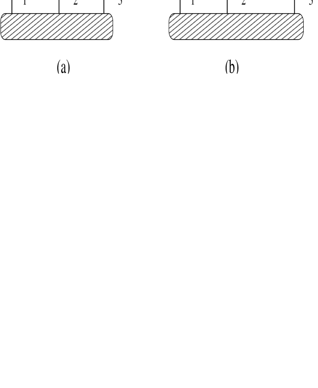
FIG. 2.: The diagrams corresponding to the pionic contributions to the current: (a) the pion-in-flight diagram, (b) the pair term. The bound state of the quarks is represented by the blobs at the beginning and the end of the diagrams.

From the 2-body operators $\mbox{\boldmath${\rm J}$}_{2b}$, (65-66) we may write down the current matrix element between the 3-quark state

$$\mbox{\boldmath${\rm M}$}_{2b}=3\mbox{\boldmath${\rm M}$}_{2b}^{(1)}=3\frac{1}{N}\int\int d^{3}pd^{3}q\bar{\Psi}\gamma_{0}^{(1)}\mbox{\boldmath${\rm J}$}_{2b}^{(23)}\Psi.$$ (69)

Taking the curl of Eq. (69) the magnetic moment can be determined. The resulting expressions are given in Appendix C. As a check using the obtained magnetic moment operators we have determined the exchange magnetic moment contribution to the trinucleon system. Our results agree with those obtained by Kloet and Tjon [33].

TABLE III.: The single quark current contribution $\mu_{N}^{(1)}$ to the magnetic moment in units of nuclear magneton, together with the two-body corrections and the anomalous correction $\delta\mu_{N}^{(1)}$ arising from the pion one-loop diagrams. Also are shown the total combined prediction of our calculations and the experimental results

N	$\mu_{N}^{(1)}$	$\mu_{N}^{(\pi\pi\gamma)}$	$\mu_{N}^{(N\bar{N}\gamma)}$	$\delta\mu_{N}^{(1)}$	$\mu_{N}^{tot}$	exp
			$\sigma=0.09~{}GeV^{2}$
p	2.81	0.20	-0.21	0.12	2.92	2.79
n	-1.87	-0.20	0.21	-0.16	-2.02	-1.91
			$\sigma=0.12~{}GeV^{2}$
p	2.44	0.19	-0.18	0.11	2.56	2.79
n	-1.63	-0.19	0.18	-0.14	-1.78	-1.91
			$\sigma=0.15~{}GeV^{2}$
p	2.20	0.18	-0.16	0.10	2.32	2.79
n	-1.46	-0.18	0.16	-0.13	-1.61	-1.91

To get an estimate of the exchange current contributions in the 3-quark case we have used for the couplings and cut off mass the values from Ref. [32]. They are taken to be $g_{qq\pi}^{2}/4\pi=0.67$. The results for the magnetic moments are shown in Table III. Our estimates are in strong disagreement with those obtained in Ref. [32]. The pion-in-flight contribution is substantially smaller than found in Ref. [32] using the chiral constituent model [34]. This may be partially due to the 3-quark wavefunction used, which has a matter radius smaller than in our case. Moreover, it contains only nonrelativistic components. The pair contribution is found to be comparable to the pion-in-flight term, leading to an almost cancellation of the mesonic current pionic contributions.

FIG. 3.: The diagrams contributing to the anomalous magnetic moment of the single quark

The presence of mesonic degrees of freedom will modify the single quark current. The resulting e.m. current operator can in general be characterized by a large number of off-shell form factors [36]-[38], which reduces to 2 when we assume that the initial and final quark is on-mass shell. Using this approximation we may estimate the resulting anomalous magnetic $\kappa$ term due to the the pionic contributions. Near $Q^{2}=0$ we have

$$J_{\mu}^{\gamma qq}=e_{q}\gamma_{\mu}+\kappa_{q}\frac{ie}{2M_{p}}\sigma_{\mu\nu}q_{\nu},$$ (70)

where $\kappa_{q}=\kappa_{s}+\kappa_{v}\tau_{z}$ for the u,d-quark. The $\kappa$ coefficients can be determined in a simple model, assuming that the loop corrections are given by only the one-loop pionic contributions to the e.m. vertex. Similarly as in the two-body current case we approximate the single quark orbital by a free quark propagation with a constituent mass given by the ground state orbital energy. With the above simplifying assumptions the calculation amounts to calculating the magnetic moment contributions of the diagrams shown in Fig. 3. Using the same cutoff mass regularization as for the two-body currents we find for the anomalous magnetic moment in units of the nuclear magneton,

$$\kappa^{(a)}=\kappa_{v}^{(a)}\tau_{z}=ig_{\pi qq}^{2}\tau_{z}\frac{4M_{p}}{3m_{q}^{3}}\int\frac{d^{4}k}{\left(2\pi\right)^{4}}\frac{4\left(p\cdot k\right)^{2}-p^{2}k^{2}}{\left[k^{2}-2pk+i\epsilon\right]\left[k^{2}-m_{\pi}^{2}+i\epsilon\right]^{2}}\left(\frac{\Lambda_{\pi}^{2}}{k^{2}-\Lambda_{\pi}^{2}}\right)^{2}\left(1+2\frac{k^{2}-m_{\pi}^{2}}{k^{2}-\Lambda_{\pi}^{2}}\right)$$ (71)

and

$$\kappa^{(b)}=\kappa_{s}^{(b)}+\kappa_{v}^{(b)}\tau_{z}=-ig_{\pi qq}^{2}\frac{1-\tau_{z}}{2}\frac{2M_{p}}{3m_{q}^{3}}\int\frac{d^{4}k}{\left(2\pi\right)^{4}}\frac{4\left(p\cdot k\right)^{2}-p^{2}k^{2}}{\left[k^{2}-2pk+i\epsilon\right]^{2}\left[k^{2}-m_{\pi}^{2}+i\epsilon\right]}\left(\frac{\Lambda_{\pi}^{2}}{k^{2}-\Lambda_{\pi}^{2}}\right)^{2},$$ (72)

where $p$ is the momentum of the quark. For details we refer to Appendix D. Eq. (71) corresponds to the coupling of the photon to the pion, Eq. (72) to the coupling of the photon to the quark.

TABLE IV.: The quark anomalous magnetic moments in units of nucleon magneton in the one-loop approximation for various string tension $\sigma$.The first set is the prediction for only the pion loops, while the second set is with both pion and kaon loops included.

$\sigma~{}(GeV^{2})$	$\kappa_{u}$	$\kappa_{d}$	$\kappa_{s}$
	pion loops
0.09	0.101	-0.160	0.0
0.12	0.092	-0.140	0.0
0.15	0.085	-0.126	0.0
	pion and kaon loops
0.09	0.132	-0.151	-0.034
0.12	0.121	-0.133	-0.032
0.15	0.112	-0.120	-0.031

In Table IV are shown the calculated anomalous magnetic moments of the u, d and s quarks for $\Lambda=675~{}MeV$ for various choices of $\sigma$. Clearly, the results depend on the constituent quark masses. These are given in Table I for the considered string tensions.

Using Eq. (57) the $\kappa$-term in Eq. (70) yields a nucleon magnetic moment correction

$$\delta\mu_{z}=3\delta\mu_{z}^{(1)}=3\left<\psi_{symm}\left|\kappa_{q}(1)\sigma_{z}(1)\right|\psi_{symm}\right>\lambda_{0}$$ (73)

with

$$\lambda_{0}=\frac{\int r^{2}dr(|g|^{2}-|f|^{2})}{\int r^{2}dr(|g|^{2}+|f|^{2})}$$ (74)

In Table III the predictions for the nucleon are shown including also the one-pion loop contributions (73) and two-body currents. Our results obtained for the one-loop corrections are smaller than reported by Glozman and Riska [39]. This is due to the inclusion of the lower component in the single quark orbitals. Neglecting these we recover the results of Ref. [39]. From Table III we see that the proton and neutron magnetic moment is in reasonable agreement with experiment for a string tension of $\sigma=0.1~{}~{}GeV^{2}$. For this value of the string tension the model predicts a nucleon mass of $940MeV$, remarkably close to the empirical value. The anomalous magnetic moment contributions are found to be of the order of 10%.

Due to the one-loop contributions the magnetic moments of the other baryons are modified. Corrections from kaon loops have also been considered. Because of the larger kaon mass the contributions are expected in general to be smaller in size than those of the pion loops. In Table IV the calculated anomalous moment of the strange quark due to the kaon one-loop corrections are given. In the calculations a cutoff mass of $\Lambda=675~{}MeV$ has been used. The isoscalar and isovector anomalous magnetic moment pieces are also changed by the kaon loop contributions. From Table IV we see that the kaon loop contributions are indeed smaller in magnitude as compared to the pion loop ones. The full results for the magnetic moments of the baryon octet and decuplet, including the pionic exchange currents and the pion and kaon one-loop contributions are summarized in Table V. For the value of the string tension $\sigma=0.1$ the overall agreement with the experimental data is reasonable. From the table we see that the anomalous magnetic moment contribution leads to an improvement of the predictions.

TABLE V.: The magnetic moment $\mu_{B}$ of the baryon octet and decuplet in units of nuclear magneton, including the anomalous contribution $\delta\mu_{B}$ arising from the pion and kaon one-loop diagrams and the pion exchange corrections for different string tension $\sigma$. Also are shown the experimental results

B	$\delta\mu_{B}$	$\mu_{B}$	$\delta\mu_{B}$	$\mu_{B}$	$\delta\mu_{B}$	$\mu_{B}$	exp
	$\sigma=0.09~{}GeV^{2}$		$\sigma=0.12~{}GeV^{2}$		$\sigma=0.15~{}GeV^{2}$
p	0.15	2.95	0.14	2.59	0.12	2.34	2.79
n	-0.16	-2.02	-0.14	-1.78	-0.13	-1.61	-1.91
$\Sigma^{-}$	-0.13	-1.16	-0.11	-1.00	-0.10	-0.89	-1.16
$\Sigma^{0}$	0.00	0.85	0.00	0.74	0.00	0.67
$\Sigma^{+}$	0.12	2.84	0.11	2.48	0.11	2.25	2.46
$\Lambda$	-0.02	-0.68	-0.02	-0.62	-0.02	-0.58	-0.61
$\Xi^{-}$	0.00	-0.57	0.00	-0.53	0.00	-0.50	-0.65
$\Xi^{0}$	-0.06	-1.57	-0.05	-1.39	-0.05	-1.28	-1.25
$\Delta^{++}$	0.26	5.88	0.24	5.13	0.22	4.61	4.52
$\Delta^{+}$	0.07	2.88	0.07	2.51	0.07	2.27
$\Delta^{0}$	-0.11	-0.11	-0.10	-0.10	-0.08	-0.08
$\Delta^{-}$	-0.30	-3.11	-0.26	-2.70	-0.24	-2.44
$\Sigma^{+*}$	0.15	3.24	0.14	2.80	0.13	2.50
$\Sigma^{0*}$	-0.04	0.23	-0.03	0.18	-0.03	0.15
$\Sigma^{-*}$	-0.22	-2.76	-0.20	-2.43	-0.18	-2.20
$\Xi^{0*}$	0.04	0.59	0.04	0.47	0.03	0.38
$\Xi^{-*}$	-0.14	-2.40	-0.13	-2.15	-0.12	-1.96
$\Omega^{-}$	-0.07	-2.06	-0.06	-1.86	-0.06	-1.73	-2.02

VII Conclusion

We have written down the general effective quark Lagrangian as obtained from the standard QCD Lagrangian by integrating out the gluonic degrees of freedom. Considering the baryon Green’s function, neglecting gluon and meson exchanges, we find in lowest order of the approximation scheme that it is given by a product of 3 independent single quark Green’s functions. As a result the Hamiltonian can be written as a sum of three quark terms, where the single quark solutions satisfy the Dyson-Schwinger equation with a nonlocal kernel.

The nonlinear equation for the single quark propagator $S$ (attached to the string in a gauge–invariant way) has been solved in the Gaussian correlator approximation. The resulting 3-quark wavefunction has been used to determine the magnetic moments of the baryons. This has been done for both the octet and decuplet of the SU(3) flavour group.

Comparing the predictions we find that the magnetic moments are mostly in close overall agreement with the experiment for a string tension of $\sigma=0.1~{}GeV^{2}$. We find, that the predicted magnetic moment of the nucleon is improved substantially once we choose a string tension to give a reasonable nucleon mass. The same applies for the $\Delta$-isobar. Effects due to the presence of virtual mesons are in general expected to be important. We have estimated the pionic one-loop and one pion exchange contributions to the magnetic moment. The single quark corrections from pionic loops are found to be of the order of 10%, whereas the total effect of 2-body current contributions are predicted to be small, to be contrasted to the results of Ref. [32]. This is due to the cancellation of the pion in flight and pair term in the present model. Because of the anomalous magnetic contributions there seems to be somewhat an improvement of the predictions.

Our results for predictions of the magnetic moments of baryons are encouraging, but are in need of including higher order corrections. In particular, the mass spectrum obtained from our lowest order approximation does not contain the $N-\Delta$ mass splitting. This is due to neglecting contributions like the hyperfine interaction arising from the one gluon interaction. It is clearly of interest to investigate how the magnetic moments are changed when effects from color Coulomb and hyperfine interaction are accounted for.

A Magnetic moment calculation in coordinate space

The one-quark contribution to the magnetic moment can be written as in (45)

$$\langle\Delta H_{1}\rangle=-e_{q}^{(1)}\int(\varphi^{(1)*}\mbox{\boldmath${\rm\sigma}$}^{(1)}\mbox{\boldmath${\rm A}$}\chi^{(1)}+\chi^{(1)*}\mbox{\boldmath${\rm\sigma}$}^{(1)}\mbox{\boldmath${\rm A}$}\varphi^{(1)})d^{3}r,$$ (A1)

where $\mbox{\boldmath${\rm A}$}=\frac{1}{2}(\mbox{\boldmath${\rm H}$}\times\mbox{\boldmath${\rm r}$})$ is the vector potential of external constant magnetic field.

Inserting in (A.1) $\varphi^{(1)}=g(r)\Omega_{jlM}$ and $\chi^{(1)}=if(r)\Omega_{jl^{\prime}M}$, and taking into account that $\Omega_{jl^{\prime}M}=-(\mbox{\boldmath${\rm\sigma}$}\mbox{\boldmath${\rm n}$})\Omega_{jlM}$, one easily obtains

$$\langle\Delta H_{1}\rangle=-\frac{1}{2}e^{(1)}_{q}\int d^{3}r(g^{*}f+f^{*}g)r\Omega^{*}_{jlM}\{(\mbox{\boldmath${\rm\sigma}$}\mbox{\boldmath${\rm n}$})(\mbox{\boldmath${\rm n}$}\mbox{\boldmath${\rm H}$})-\mbox{\boldmath${\rm\sigma}$}\mbox{\boldmath${\rm H}$}\}\Omega_{jlM}$$ (A2)

Eq.(A.2) contains the matrix element $\int d\mbox{\boldmath${\rm n}$}\Omega^{*}_{jlM}n_{i}n_{k}\Omega_{jlM}$, which simplifies when $l=0$, so that $\langle n_{i}n_{k}\rangle=\frac{1}{3}\delta_{ik}$.

In this case one obtains, taking into account relation $\langle\Delta H_{1}\rangle=\Delta E=-\mbox{\boldmath${\rm\mu}$}^{(1)}\mbox{\boldmath${\rm H}$}$,

$$\mbox{\boldmath${\rm\mu}$}^{(1)}=-\frac{1}{3}e^{(1)}_{q}\int(g^{*}(r)f(r)+f^{*}(r)g(r))rd^{3}r\Omega^{*}_{jlM}\mbox{\boldmath${\rm\sigma}$}^{(1)}\Omega_{jlM}=$$

$$=-\mbox{\boldmath${\rm\sigma}$}^{(1)}\frac{2}{3}e^{(1)}_{q}\int Re(g^{*}(r)f(r))r^{3}dr$$ (A3)

In the case of a local scalar potential $U(r)$ one can further express $f(r)$ through $g(r)$ using the Dirac equation for the one-quark state

$$rf(r)=\frac{1}{\varepsilon+m+U(r)}\left(\frac{d}{dr}(gr)+\frac{\kappa}{r}gr\right)$$ (A4)

Introducing (A.4) into (A.3) and integrating by parts one obtains

$$\mu^{(i)}_{z}=\frac{e_{q}^{(i)}\sigma_{z}^{(i)}}{3}\int\frac{|g|^{2}r^{2}dr}{(\varepsilon+m+U)^{2}}(3(\varepsilon+m+U)-rU^{\prime}(r))$$ (A5)

For $U(r)=\sigma r$ one obtains Eq.(49).

B Magnetic moment of the multiplet

In this Appendix the calculation of the nucleon magnetic moment is generalized to the baryon octet and decuplet. By analogy with the fully symmetrical $3q$ wave function for the nucleon, Eqs. (46-47), wave functions for the baryon multiplets can be formulated. The flavor octet with total spin $1/2$ up becomes,

$$\Psi^{p}_{symm} = \frac{\sqrt{2}}{6}\left\{2d_{-}u_{+}u_{+}-u_{-}d_{+}u_{+}-d_{+}u_{-}u_{+}+2u_{+}d_{-}u_{+}\right.$$ (B2)

$$\left.-u_{+}u_{-}d_{+}-u_{-}u_{+}d_{+}-u_{+}d_{+}u_{-}-d_{+}u_{+}u_{-}+2u_{+}u_{+}d_{-}\right\},$$

$$\Psi^{n}_{symm} = \frac{\sqrt{2}}{6}\left\{2u_{-}d_{+}d_{+}-d_{-}u_{+}d_{+}-u_{+}d_{-}d_{+}+2d_{+}u_{-}d_{+}\right.$$ (B4)

$$\left.-d_{+}d_{-}u_{+}-d_{-}d_{+}u_{+}-d_{+}u_{+}d_{-}-u_{+}d_{+}d_{-}+2d_{+}d_{+}u_{-}\right\},$$

$$\Psi^{\Sigma^{+}}_{symm} = \frac{\sqrt{2}}{6}\left\{2s_{-}u_{+}u_{+}-u_{-}s_{+}u_{+}-s_{+}u_{-}u_{+}+2u_{+}s_{-}u_{+}\right.$$ (B6)

$$\left.-u_{+}u_{-}s_{+}-u_{-}u_{+}s_{+}-u_{+}s_{+}u_{-}-s_{+}u_{+}u_{-}+2u_{+}u_{+}s_{-}\right\},$$

$$\Psi^{\Sigma^{0}}_{symm} = \frac{-1}{6}\left\{u_{+}d_{-}s_{+}+d_{+}u_{-}s_{+}+s_{+}d_{-}u_{+}+s_{+}u_{-}d_{+}-2u_{+}s_{-}d_{+}-2d_{+}s_{-}u_{+}\right.$$ (B9)

$$\left.+u_{-}d_{+}s_{+}+d_{-}u_{+}s_{+}-2s_{-}d_{+}u_{+}-2s_{-}u_{+}d_{+}+u_{-}s_{+}d_{+}+d_{-}s_{+}u_{+}\right.$$

$$\left.-2u_{+}d_{+}s_{-}-2d_{+}u_{+}s_{-}+s_{+}d_{+}u_{-}+s_{+}u_{+}d_{-}+u_{+}s_{+}d_{-}+d_{+}s_{+}u_{-}\right\},$$

$$\Psi^{\Sigma^{-}}_{symm} = \frac{\sqrt{2}}{6}\left\{2s_{-}d_{+}d_{+}-d_{-}s_{+}d_{+}-s_{+}d_{-}d_{+}+2d_{+}s_{-}d_{+}\right.$$ (B11)

$$\left.-d_{+}d_{-}s_{+}-d_{-}d_{+}s_{+}-d_{+}s_{+}d_{-}-s_{+}d_{+}d_{-}+2d_{+}d_{+}s_{-}\right\},$$

$$\Psi^{\Lambda}_{symm} = \frac{\sqrt{3}}{6}\left\{u_{-}d_{+}s_{+}-d_{-}u_{+}s_{+}+u_{-}s_{+}d_{+}-d_{-}s_{+}u_{+}-u_{+}d_{-}s_{+}+d_{+}u_{-}s_{+}\right.$$ (B13)

$$\left.-s_{+}d_{-}u_{+}+s_{+}u_{-}d_{+}+s_{+}d_{+}u_{-}-s_{+}u_{+}d_{-}-u_{+}s_{+}d_{-}+d_{+}s_{+}u_{-}\right\},$$

$$\Psi^{\Xi^{0}}_{symm} = \frac{\sqrt{2}}{6}\left\{2u_{-}s_{+}s_{+}-s_{-}u_{+}s_{+}-u_{+}s_{-}s_{+}+2s_{+}u_{-}s_{+}\right.$$ (B15)

$$\left.-s_{+}s_{-}u_{+}-s_{-}s_{+}u_{+}-s_{+}u_{+}s_{-}-u_{+}s_{+}s_{-}+2s_{+}s_{+}u_{-}\right\},$$

$$\Psi^{\Xi^{-}}_{symm} = \frac{\sqrt{2}}{6}\left\{2d_{-}s_{+}s_{+}-s_{-}d_{+}s_{+}-d_{+}s_{-}s_{+}+2s_{+}d_{-}s_{+}\right.$$ (B17)

$$\left.-s_{+}s_{-}d_{+}-s_{-}s_{+}d_{+}-s_{+}d_{+}s_{-}-d_{+}s_{+}s_{-}+2s_{+}s_{+}d_{-}\right\},$$

where the subscripts ($\pm$) refer to the spin projection. For the flavor decuplet with total spin $3/2$ up we have

$$\Psi^{\Delta^{++}}_{symm} = u_{+}u_{+}u_{+},$$ (B18)

$$\Psi^{\Delta^{+}}_{symm} = \frac{1}{\sqrt{3}}\left\{u_{+}u_{+}d_{+}+u_{+}d_{+}u_{+}+d_{+}u_{+}u_{+}\right\},$$ (B19)

$$\Psi^{\Delta^{0}}_{symm} = \frac{1}{\sqrt{3}}\left\{d_{+}d_{+}u_{+}+d_{+}u_{+}d_{+}+u_{+}d_{+}d_{+}\right\},$$ (B20)

$$\Psi^{\Delta^{-}}_{symm} = d_{+}d_{+}d_{+},$$ (B21)

$$\Psi^{\Sigma^{+}}_{symm} = \frac{1}{\sqrt{3}}\left\{u_{+}u_{+}s_{+}+u_{+}s_{+}u_{+}+s_{+}u_{+}u_{+}\right\},$$ (B22)

$$\Psi^{\Sigma^{0}}_{symm} = \frac{1}{\sqrt{6}}\left\{u_{+}d_{+}s_{+}+d_{+}u_{+}s_{+}+u_{+}s_{+}d_{+}+s_{+}u_{+}d_{+}+d_{+}s_{+}u_{+}+s_{+}d_{+}u_{+}\right\},$$ (B23)

$$\Psi^{\Sigma^{-}}_{symm} = \frac{1}{\sqrt{3}}\left\{d_{+}d_{+}s_{+}+d_{+}s_{+}d_{+}+s_{+}d_{+}d_{+}\right\},$$ (B24)

$$\Psi^{\Xi^{0}_{symm}} = \frac{1}{\sqrt{3}}\left\{s_{+}s_{+}u_{+}+s_{+}u_{+}s_{+}+u_{+}s_{+}s_{+}\right\},$$ (B25)

$$\Psi^{\Xi^{-}}_{symm} = \frac{1}{\sqrt{3}}\left\{s_{+}s_{+}d_{+}+s_{+}d_{+}s_{+}+d_{+}s_{+}s_{+}\right\},$$ (B26)

$$\Psi^{\Omega^{-}}_{symm} = s_{+}s_{+}s_{+}.$$ (B27)

These fully symmetrical wave functions Eqs. (B2)-(B27) can be written symbolically as,

$$\psi^{N}_{JM,symm}=\Gamma^{\alpha\beta\gamma}_{JM}(f_{1}f_{2}f_{3})\psi^{f_{1}}_{\alpha}\psi^{f_{2}}_{\beta}\psi^{f_{3}}_{\gamma}.$$ (B28)

As the orbital of the $s$-quark is heavier than the $u$- and $d$-quark orbitals Eq. (51) has to be split up in contributions from the $u,d$-quark and from the $s$-quark. Using the symmetrical wavefunction Eq. (B28) this is realized by writing,

$$\mu_{z}=3\mu_{z}^{(1)}=3\sum_{f_{1}f_{2}f_{3}}\left<\Gamma^{\alpha\beta\gamma}_{JM}(f_{1}f_{2}f_{3})\psi^{f_{1}}_{\alpha}\psi^{f_{2}}_{\beta}\psi^{f_{3}}_{\gamma}\left|e_{q}(1)\sigma_{z}(1)\right|\Gamma^{\alpha\beta\gamma}_{JM}(f_{1}f_{2}f_{3})\psi^{f_{1}}_{\alpha}\psi^{f_{2}}_{\beta}\psi^{f_{3}}_{\gamma}\right>{\lambda}_{f_{1}},$$ (B29)

with,

$${\lambda}_{f_{i}}=-\frac{2}{3}\int g_{f_{i}}^{*}(r)f_{f_{i}}(r)r^{3}dr.$$ (B30)

The flavor index $f_{i}$ can take the values $u,d$ or $s$. Note that $\lambda_{u}=\lambda_{d}$ as the same orbital is taken for the $u$- and $d$-quark. Evaluating Eq. (B29) for the different baryon wave functions Eqs. (B2-B27) results in the expressions in Table VI.

TABLE VI.: The matrix elements of the e.m. current for the baryons.

N	$\mu_{N}/3$
p	$\frac{1}{3}{\lambda}_{u}$
n	$-\frac{2}{9}{\lambda}_{u}$
$\Sigma^{+}$	$\frac{8}{27}{\lambda}_{u}+\frac{1}{27}{\lambda}_{s}$
$\Sigma^{0}$	$\frac{2}{27}{\lambda}_{u}+\frac{1}{27}{\lambda}_{s}$
$\Sigma^{-}$	$-\frac{4}{27}{\lambda}_{u}+\frac{1}{27}{\lambda}_{s}$
$\Lambda$	$-\frac{1}{9}{\lambda}_{s}$
$\Xi^{0}$	$-\frac{4}{27}{\lambda}_{s}-\frac{2}{27}{\lambda}_{u}$
$\Xi^{-}$	$-\frac{4}{27}{\lambda}_{s}+\frac{1}{27}{\lambda}_{u}$
$\Delta^{++}$	$\frac{2}{3}{\lambda}_{u}$
$\Delta^{+}$	$\frac{1}{3}{\lambda}_{u}$
$\Delta^{0}$	$0$
$\Delta^{-}$	$-\frac{1}{3}{\lambda}_{u}$
$\Sigma^{+*}$	$\frac{4}{9}{\lambda}_{u}-\frac{1}{9}{\lambda}_{s}$
$\Sigma^{0*}$	$\frac{1}{9}{\lambda}_{u}-\frac{1}{9}{\lambda}_{s}$
$\Sigma^{-*}$	$-\frac{2}{9}{\lambda}_{u}-\frac{1}{9}{\lambda}_{s}$
$\Xi^{0*}$	$-\frac{2}{9}{\lambda}_{s}+\frac{2}{9}{\lambda}_{u}$
$\Xi^{-*}$	$-\frac{2}{9}{\lambda}_{s}-\frac{1}{9}{\lambda}_{u}$
$\Omega^{-}$	$-\frac{1}{3}{\lambda}_{s}$

C Pionic two-body contribution to the magnetic moment

In this Appendix the pion-in-flight and pair contributions to the magnetic moment of the nucleons are given. Following Ref. [33] these contributions are determined by taking the curl of the pionic two-body currents Eq. (69). The 3-quark state $\Psi$ is given by the product of three single quark orbitals Eq. (35). Because of symmetry considerations it suffices to calculate the magnetic moment contribution of pion exchange between say the second and the third quark only and multiply the result by a factor of 3 to include the contribution of the other possible permutations of quark pairs.

Considering the pion-in-flight contribution first (Eq. (65)), taking the curl gives rather long expressions which can be divided into two parts,

$$\delta\mu_{z}^{proton}=-\delta\mu_{z}^{neutron}=3\left(\delta\mu_{z}^{A}+3\delta\mu_{z}^{B}\right).$$ (C1)

The first part gives the larger contribution and can be written as,

$$\delta\mu_{z}^{A} = \lim_{Q^{2}\rightarrow 0}\frac{2eg_{\pi qq}^{2}}{3(2\pi)^{3}N}\int d^{3}qd^{3}pd^{3}p^{\prime}\frac{1}{(\mbox{\boldmath${\rm\Delta}$}^{2}+m_{\pi}^{2})^{2}}\left(|\tilde{g}(k_{1})|^{2}+|\tilde{f}(k_{1})|^{2}\right)\times$$ (C7)

$$\left\{\tilde{g}(k^{\prime}_{2})\tilde{f}(k_{2})\tilde{g}(k^{\prime}_{3})\tilde{f}(k_{3})\frac{1}{3k_{2}k_{3}}\left(\mbox{\boldmath${\rm p}$}\mbox{\boldmath${\rm\Delta}$}-p_{z}\Delta_{z}\right)\right.$$

$$+\tilde{g}(k^{\prime}_{2})\tilde{f}(k_{2})\tilde{f}(k^{\prime}_{3})\tilde{g}(k_{3})\frac{1}{6k_{2}k^{\prime}_{3}}\left((2\mbox{\boldmath${\rm p}$}-\mbox{\boldmath${\rm p}$}^{\prime}+\sqrt{3}\mbox{\boldmath${\rm q}$})\mbox{\boldmath${\rm\Delta}$}-(2p_{z}-p^{\prime}_{z}+\sqrt{3}q_{z})\Delta_{z}\right)$$

$$+\tilde{f}(k^{\prime}_{2})\tilde{g}(k_{2})\tilde{g}(k^{\prime}_{3})\tilde{f}(k_{3})\frac{1}{6k^{\prime}_{2}k_{3}}\left((2\mbox{\boldmath${\rm p}$}-\mbox{\boldmath${\rm p}$}^{\prime}-\sqrt{3}\mbox{\boldmath${\rm q}$})\mbox{\boldmath${\rm\Delta}$}-(2p_{z}-p^{\prime}_{z}-\sqrt{3}q_{z})\Delta_{z}\right)$$

$$\left.+\tilde{f}(k^{\prime}_{2})\tilde{g}(k_{2})\tilde{f}(k^{\prime}_{3})\tilde{g}(k_{3})\frac{-2}{3k^{\prime}_{2}k^{\prime}_{3}}\left(\mbox{\boldmath${\rm p}$}^{\prime}\mbox{\boldmath${\rm\Delta}$}-p^{\prime}_{z}\Delta_{z}\right)\right\}\times$$

$$\left(1+2\frac{\mbox{\boldmath${\rm\Delta}$}^{2}+m_{\pi}^{2}}{\mbox{\boldmath${\rm\Delta}$}^{2}+\Lambda_{\pi}^{2}}\right)\left(\frac{\Lambda_{\pi}^{2}}{\mbox{\boldmath${\rm\Delta}$}^{2}+\Lambda_{\pi}^{2}}\right)^{2}.$$

The second part comes from the curl applied to the wavefunctions

$$\delta\mu_{z}^{B} = \lim_{Q^{2}\rightarrow 0}\frac{2eg_{\pi qq}^{2}}{3(2\pi)^{3}N}\int d^{3}qd^{3}pd^{3}p^{\prime}\frac{1}{(\mbox{\boldmath${\rm\Delta}$}^{2}+\mu^{2})^{2}}\left(|\tilde{g}(k_{1})|^{2}+|\tilde{f}(k_{1})|^{2}\right)\frac{1}{3}\left(\hat{\mbox{\boldmath${\rm k}$}}^{\prime}_{2}\times\mbox{\boldmath${\rm\Delta}$}\right)_{z}$$ (C12)

$$\left\{\frac{\partial\tilde{g}(k^{\prime}_{2})}{\partial k^{\prime}_{2}}\tilde{f}(k_{2})\tilde{g}(k^{\prime}_{3})\tilde{f}(k_{3})\left(\hat{\mbox{\boldmath${\rm k}$}}_{2}\times\hat{\mbox{\boldmath${\rm k}$}}_{3}\right)_{z}-\frac{\partial\tilde{g}(k^{\prime}_{2})}{\partial k^{\prime}_{2}}\tilde{f}(k_{2})\tilde{f}(k^{\prime}_{3})\tilde{g}(k_{3})\left(\hat{\mbox{\boldmath${\rm k}$}}_{2}\times\hat{\mbox{\boldmath${\rm k}$}}^{\prime}_{3}\right)_{z}\right.$$

$$-\frac{\partial\tilde{f}(k^{\prime}_{2})}{\partial k^{\prime}_{2}}\tilde{g}(k_{2})\tilde{g}(k^{\prime}_{3})\tilde{f}(k_{3})\left(\hat{\mbox{\boldmath${\rm k}$}}^{\prime}_{2}\times\hat{\mbox{\boldmath${\rm k}$}}_{3}\right)_{z}+\frac{\partial\tilde{f}(k^{\prime}_{2})}{\partial k^{\prime}_{2}}\tilde{g}(k_{2})\tilde{f}(k^{\prime}_{3})\tilde{g}(k_{3})\left(\hat{\mbox{\boldmath${\rm k}$}}^{\prime}_{2}\times\hat{\mbox{\boldmath${\rm k}$}}^{\prime}_{3}\right)_{z}$$

$$+\tilde{f}(k^{\prime}_{2})\tilde{g}(k_{2})\tilde{g}(k^{\prime}_{3})\tilde{f}(k_{3})\frac{1}{k^{\prime}_{2}}\left(\hat{\mbox{\boldmath${\rm k}$}}^{\prime}_{2}\times\hat{\mbox{\boldmath${\rm k}$}}_{3}\right)_{z}\left.-\tilde{f}(k^{\prime}_{2})\tilde{g}(k_{2})\tilde{f}(k^{\prime}_{3})\tilde{g}(k_{3})\frac{1}{k^{\prime}_{2}}\left(\hat{\mbox{\boldmath${\rm k}$}}^{\prime}_{2}\times\hat{\mbox{\boldmath${\rm k}$}}^{\prime}_{3}\right)_{z}\right\}$$

$$\times\left(1+2\frac{\mbox{\boldmath${\rm\Delta}$}^{2}+m_{\pi}^{2}}{\mbox{\boldmath${\rm\Delta}$}^{2}+\Lambda_{\pi}^{2}}\right)\left(\frac{\Lambda_{\pi}^{2}}{\mbox{\boldmath${\rm\Delta}$}^{2}+\Lambda_{\pi}^{2}}\right)^{2}.$$

The normalization factor $N$ is the same as used before in the single quark current contribution (Eq. (62)). The momenta are expressed in terms of the Jacobi coordinates Eqs. (63) again, but from imposing the Breit system and momentum conservation we now get $\mbox{\boldmath${\rm P}$}^{\prime}=-\mbox{\boldmath${\rm P}$}=\mbox{\boldmath${\rm Q}$}/2$ and $2\sqrt{3}(\mbox{\boldmath${\rm q}$}^{\prime}-\mbox{\boldmath${\rm q}$})=\mbox{\boldmath${\rm Q}$}$. In writing down these expressions use has been made of the spin-isospin operator sandwiched between the fully symmetric wavefunctions in spin-isospin and orbital space of the 3 quarks,

$$\begin{array}[]{c}\left<\psi_{symm}^{p}\left|\left(\mbox{\boldmath${\rm\tau}$}^{(1)}\times\mbox{\boldmath${\rm\tau}$}^{(2)}\right)_{z}\sigma^{(1)}_{i}\sigma^{(2)}_{j}\right|\psi_{symm}^{p}\right>=-\left<\psi_{symm}^{n}\left|\left(\mbox{\boldmath${\rm\tau}$}^{(1)}\times\mbox{\boldmath${\rm\tau}$}^{(2)}\right)_{z}\sigma^{(1)}_{i}\sigma^{(2)}_{j}\right|\psi_{symm}^{n}\right>\\ =-\frac{2}{3}\epsilon_{ij3}.\end{array}$$ (C13)

It should be noted that the spin-isospin factor (C13) is identical to that found for the tri-nucleon case. For all the other baryon wavefunctions given in Appendix B the matrix element of the considered two-body e.m. operators vanish, because of the isospin structure of the e.m. operator. Hence the considered two-body currents contribute only to the magnetic moment of the proton and neutron.

The second part $\delta\mu^{B}_{z}$ is a relativistic effect which enlarges the values by about 10% and which vanishes in the static limit as is shown at the end of this section.

In the same way the pair term can be analyzed. We find

$$\delta\mu^{proton}_{z}=-\delta\mu^{neutron}_{z}=3\left(\delta\mu_{z}^{C}+3\delta\mu_{z}^{D}\right)$$ (C14)

with

$$\delta\mu_{z}^{C} = \lim_{Q^{2}\rightarrow 0}\frac{eg_{\pi qq}^{2}}{2m_{q}(2\pi)^{3}N}\int d^{3}qd^{3}pd^{3}p^{\prime}\frac{1}{\mbox{\boldmath${\rm\Delta}$}^{2}+m_{\pi}^{2}}\frac{1}{3}\left(|\tilde{g}(k_{1})|^{2}+|\tilde{f}(k_{1})|^{2}\right)$$ (C19)

$$\left\{\frac{1}{k_{2}}\left(\frac{1}{3}-\frac{\mbox{\boldmath${\rm\Delta}$}\mbox{\boldmath${\rm k}$}_{2}-\Delta_{z}(k_{2})_{z}}{\Delta^{2}+m_{\pi}^{2}}\right)\tilde{g}(k^{\prime}_{2})\tilde{f}(k_{2})\tilde{g}(k^{\prime}_{3})\tilde{g}(k_{3})\right.$$

$$+\frac{1}{k^{\prime}_{2}}\left(\frac{2}{3}+\frac{\mbox{\boldmath${\rm\Delta}$}\mbox{\boldmath${\rm k}$}^{\prime}_{2}-\Delta_{z}(k^{\prime}_{2})_{z}}{\Delta^{2}+m_{\pi}^{2}}\right)\tilde{f}(k^{\prime}_{2})\tilde{g}(k_{2})\tilde{g}(k^{\prime}_{3})\tilde{g}(k_{3})$$

$$+\frac{1}{k_{3}}\left(\frac{1}{3}+\frac{\mbox{\boldmath${\rm\Delta}$}\mbox{\boldmath${\rm k}$}_{3}-\Delta_{z}(k_{3})_{z}}{\Delta^{2}+m_{\pi}^{2}}\right)\tilde{g}(k^{\prime}_{2})\tilde{g}(k_{2})\tilde{g}(k^{\prime}_{3})\tilde{f}(k_{3})$$

$$\left.+\frac{1}{k^{\prime}_{3}}\left(\frac{2}{3}-\frac{\mbox{\boldmath${\rm\Delta}$}\mbox{\boldmath${\rm k}$}^{\prime}_{3}-\Delta_{z}(k^{\prime}_{3})_{z}}{\mbox{\boldmath${\rm\Delta}$}^{2}+m_{\pi}^{2}}\right)\tilde{g}(k^{\prime}_{2})\tilde{g}(k_{2})\tilde{f}(k^{\prime}_{3})\tilde{g}(k_{3})\right\}\left(\frac{\Lambda_{\pi}^{2}}{\mbox{\boldmath${\rm\Delta}$}^{2}+\Lambda_{\pi}^{2}}\right)^{2}$$

and

$$\delta\mu_{z}^{D} = \lim_{Q^{2}\rightarrow 0}\frac{eg_{\pi qq}^{2}}{6m_{q}(2\pi)^{3}N}\int\int\int d^{3}qd^{3}pd^{3}p^{\prime}\frac{1}{\mbox{\boldmath${\rm\Delta}$}^{2}+m_{\pi}^{2}}\frac{1}{3}\left(|\tilde{g}(k_{1})|^{2}+|\tilde{f}(k_{1})|^{2}\right)$$ (C23)

$$\left\{\frac{\partial\tilde{g}(k^{\prime}_{2})}{\partial k^{\prime}_{2}}\tilde{g}(k_{2})\left(\tilde{g}(k^{\prime}_{3})\tilde{f}(k_{3})\left(\hat{\mbox{\boldmath${\rm k}$}}^{\prime}_{2}\hat{\mbox{\boldmath${\rm k}$}}_{3}-(\hat{k}^{\prime}_{2})_{z}(\hat{k}_{3})_{z}\right)-\tilde{f}(k^{\prime}_{3})\tilde{g}(k_{3})\left(\hat{\mbox{\boldmath${\rm k}$}}^{\prime}_{2}\hat{\mbox{\boldmath${\rm k}$}}^{\prime}_{3}-(\hat{k}^{\prime}_{2})_{z}(\hat{k}^{\prime}_{3})_{z}\right)\right)\right.$$

$$+\tilde{g}(k^{\prime}_{3})\tilde{g}(k_{3})\left(-\frac{\partial\tilde{g}(k^{\prime}_{2})}{\partial k^{\prime}_{2}}\tilde{f}(k_{2})\left(\hat{\mbox{\boldmath${\rm k}$}}^{\prime}_{2}\hat{\mbox{\boldmath${\rm k}$}}_{2}-(\hat{k}^{\prime}_{2})_{z}(\hat{k}_{2})_{z}\right)+\frac{\partial\tilde{f}(k^{\prime}_{2})}{\partial k^{\prime}_{2}}\tilde{g}(k_{2})\left(\hat{\mbox{\boldmath${\rm k}$}}^{\prime}_{2}\hat{\mbox{\boldmath${\rm k}$}}^{\prime}_{2}-(\hat{k}^{\prime}_{2})_{z}(\hat{k}^{\prime}_{2})_{z}\right)\right)$$

$$-\left.\tilde{f}(k^{\prime}_{2})\tilde{g}(k_{2})\tilde{g}(k^{\prime}_{3})\tilde{g}(k_{3})\frac{1}{k^{\prime}_{2}}\left(\hat{\mbox{\boldmath${\rm k}$}}^{\prime}_{2}\hat{\mbox{\boldmath${\rm k}$}}^{\prime}_{2}-(\hat{k}^{\prime}_{2})_{z}(\hat{k}^{\prime}_{2})_{z}\right)\right\}\left(\frac{\Lambda_{\pi}^{2}}{\mbox{\boldmath${\rm\Delta}$}^{2}+\Lambda_{\pi}^{2}}\right)^{2}.$$

In the non-relativistic limit the lower component of the wavefunction can be expressed in the upper component as

$$\tilde{f}(k)=-\frac{|k|}{2m_{q}}\tilde{g}(k),$$ (C24)

where $m_{q}$ is the constituent mass of the quark. As a result, the pionic two-body current contributions Eqs. (C1-C12) and Eqs. (C14-C23) can be simplified considerably. We obtain for the pion-in-flight contribution

$$\begin{array}[]{c}\delta\mu^{A}_{z}=\frac{eg_{\pi qq}^{2}}{6m_{q}^{2}(2\pi)^{3}N}\int d^{3}qd^{3}pd^{3}p^{\prime}\left(|\tilde{g}(k_{1})|^{2}+|\tilde{f}(k_{1})|^{2}\right)\tilde{g}(k^{\prime}_{2})\tilde{g}(k_{2})\tilde{g}(k^{\prime}_{3})\tilde{g}(k_{3})\\ \frac{\mbox{\boldmath${\rm\Delta}$}^{2}-\Delta_{z}\Delta_{z}}{\left(\mbox{\boldmath${\rm\Delta}$}^{2}+m_{\pi}^{2}\right)^{2}}\left(1+2\frac{\mbox{\boldmath${\rm\Delta}$}^{2}+m_{\pi}^{2}}{\mbox{\boldmath${\rm\Delta}$}^{2}+\Lambda_{\pi}^{2}}\right).\left(\frac{\Lambda_{\pi}^{2}}{\mbox{\boldmath${\rm\Delta}$}^{2}+\Lambda_{\pi}^{2}}\right)^{2}.\end{array}$$ (C25)

For the pair term we get

$$\begin{array}[]{c}\delta\mu^{C}_{z}=\frac{eg_{\pi qq}^{2}}{6m_{q}^{2}(2\pi)^{3}N}\int d^{3}qd^{3}pd^{3}p^{\prime}\left(|\tilde{g}(k_{1})|^{2}+|\tilde{f}(k_{1})|^{2}\right)\tilde{g}(k^{\prime}_{2})\tilde{g}(k_{2})\tilde{g}(k^{\prime}_{3})\tilde{g}(k_{3})\\ \left(\frac{\mbox{\boldmath${\rm\Delta}$}^{2}-\Delta_{z}^{2}}{\left(\mbox{\boldmath${\rm\Delta}$}^{2}+m_{\pi}^{2}\right)^{2}}-\frac{1}{\mbox{\boldmath${\rm\Delta}$}^{2}+m_{\pi}^{2}}\right)\left(\frac{\Lambda_{\pi}^{2}}{\mbox{\boldmath${\rm\Delta}$}^{2}+\Lambda_{\pi}^{2}}\right)^{2},\end{array}$$ (C26)

while $\delta\mu^{B}_{z}$ and $\delta\mu^{D}_{z}$ vanish. These expressions agree with the results of Refs. [33] and [35].

D Anomalous magnetic moment contributions from pion loops

Our starting point is the e.m. currents, corresponding to the one-loop diagrams shown in Fig. 3,

$$J_{\mu}^{(a)} = -2ig_{\pi qq}^{2}e\tau_{z}\int\frac{d^{4}k}{\left(2\pi\right)^{4}}\frac{\gamma_{5}\left(\not p-\not k+m_{q}\right)\gamma_{5}\left(2k_{\mu}+Q_{\mu}\right)}{\left[(p-k)^{2}-m_{q}^{2}+i\epsilon\right]\left[k^{2}-m_{\pi}^{2}+i\epsilon\right]\left[\left(k+Q\right)^{2}-m_{\pi}^{2}+i\epsilon\right]}$$ (D2)

$$\frac{\Lambda_{\pi}^{2}}{k^{2}-\Lambda_{\pi}^{2}}\frac{\Lambda_{\pi}^{2}}{\left(k+Q\right)^{2}-\Lambda_{\pi}^{2}}\left(1+\frac{k^{2}-m_{\pi}^{2}}{\left(k+Q\right)^{2}-\Lambda_{\pi}^{2}}+\frac{\left(k+Q\right)^{2}-m_{\pi}^{2}}{k^{2}-\Lambda_{\pi}^{2}}\right)$$

and

$$J_{\mu}^{(b)}=-ig_{\pi qq}^{2}e\frac{1-\tau_{z}}{2}\int\frac{d^{4}k}{\left(2\pi\right)^{4}}.\frac{\gamma_{5}\left(\not p^{\prime}-\not k+m_{q}\right)\gamma_{\mu}\left(\not p-\not k+m_{q}\right)\gamma_{5}}{\left[(p^{\prime}-k)^{2}-m_{q}^{2}+i\epsilon\right]\left[(p-k)^{2}-m_{q}^{2}+i\epsilon\right]\left[k^{2}-m_{\pi}^{2}+i\epsilon\right]}\left(\frac{\Lambda_{\pi}^{2}}{k^{2}-\Lambda_{\pi}^{2}}\right)^{2}$$ (D3)

Since we have assumed a finite form factor at the $\pi qq$ vertex, similar as in the two-body current case, the two additional terms are needed in the last factor of Eq. (D2) to satisfy current conservation. ¿From these currents the anomalous magnetic moment has to be extracted. By applying the Gordon decomposition to the current Eq. (70) near $Q^{2}=0$ it can be seen that the anomalous magnetic moment $\kappa$ is the term proportional to $-\frac{e}{2M}K_{\mu}$ with $K_{\mu}=p_{\mu}+p^{\prime}_{\mu}$. To isolate this term the currents are rewritten by explicit evaluation of the $\gamma$-matrix algebra and taking the limit $Q^{2}\to 0$. Using the approximation that the initial and final quark is on-mass shell we obtain

$$J_{\mu}^{(a)} = -2ig_{\pi qq}^{2}e\tau_{z}\gamma^{\nu}\int\frac{d^{4}k}{\left(2\pi\right)^{4}}\frac{2k_{\mu}k_{\nu}}{\left[k^{2}-2pk+i\epsilon\right]\left[k^{2}-m_{\pi}^{2}+i\epsilon\right]^{2}}\left(\frac{\Lambda_{\pi}^{2}}{k^{2}-\Lambda_{\pi}^{2}}\right)^{2}\left(1+2\frac{k^{2}-m_{\pi}^{2}}{k^{2}-\Lambda_{\pi}^{2}}\right)$$ (D4)

$$\equiv -2ig_{\pi qq}^{2}e\tau_{z}\gamma^{\nu}C_{\mu\nu}^{(a)},$$ (D5)

and

$$J_{\mu}^{(b)} = ig_{\pi qq}^{2}e\frac{1-\tau_{z}}{2}\gamma^{\nu}\int\frac{d^{4}k}{\left(2\pi\right)^{4}}\frac{2k_{\mu}k_{\nu}-k^{2}g_{\mu\nu}}{\left[k^{2}-2pk+i\epsilon\right]^{2}\left[k^{2}-m_{\pi}^{2}+i\epsilon\right]}\left(\frac{\Lambda_{\pi}^{2}}{k^{2}-\Lambda_{\pi}^{2}}\right)^{2}$$ (D6)

$$\equiv ig_{\pi qq}^{2}e\frac{1-\tau_{z}}{2}\gamma^{\nu}C_{\mu\nu}^{(b)}.$$ (D7)

As the tensors $C^{\mu\nu}$ depend only on the initial and final momenta they can be written as,

$$C_{\mu\nu}^{(i)}=A_{1}^{(i)}K_{\mu}K_{\nu}+A_{2}^{(i)}K_{\mu}Q_{\nu}+A_{3}^{(i)}Q_{\mu}K_{\nu}+A_{4}^{(i)}Q_{\mu}Q_{\nu}+A_{5}^{(i)}g_{\mu\nu},$$ (D8)

where $A_{n}^{(i)}$ are Lorentz invariants. It can readily be seen, that only the first term $A_{1}^{(i)}$ contributes to the magnetic moment. Substituting Eq. (D8) in Eqs. (D5-D7) and taking the initial and final quark on-mass shell we find for the anomalous magnetic moment corrections

$$\kappa^{(a)}=8iM_{p}m_{q}g_{\pi qq}^{2}\tau_{z}A_{1}^{(a)},$$ (D9)

$$\kappa^{(b)}=-4iM_{p}m_{q}g_{\pi qq}^{2}\frac{1-\tau_{z}}{2}A_{1}^{(b)}.$$ (D10)

The Lorentz invariant expression $A_{1}^{(i)}$ can immediately be determined from the tensor $C_{\mu\nu}^{(i)}$. We get

$$A_{1}^{(i)}=\frac{1}{3K^{4}}\left(4K^{\mu}K^{\nu}-K^{2}g^{\mu\nu}\right)C_{\mu\nu}^{(i)}.$$ (D11)

Inserting Eq. (D11) in (D9-D10) the expressions (71-72) are obtained.

The kaon one-loop diagrams can be calculated in similar way. The starting point is the expressions Eqs. (D2-D3) again, where the mass of the pion is replaced by the mass of the kaon and the isospin structure is changed to $(\tau_{z}+3Y)/2$ and $-(\frac{2}{9}+\frac{4}{3}Y)$ respectively in Eqs. (D2-D3) with $Y$ the hypercharge. The expressions for the anomalous magnetic moment due to the kaon loop become,

$$\kappa^{(a)}=ig_{Kqq}^{2}\left(\tau_{z}+3Y\right)\frac{2M_{p}}{3m_{q}^{3}}\int\frac{d^{4}k}{\left(2\pi\right)^{4}}\frac{4\left(p\cdot k\right)^{2}-p^{2}k^{2}+3m_{q}\left(M_{q}-m_{q}\right)p\cdot k}{\left[k^{2}-2pk+m_{q}^{2}-M_{q}^{2}+i\epsilon\right]\left[k^{2}-m_{K}^{2}+i\epsilon\right]^{2}}\left(\frac{\Lambda_{K}^{2}}{k^{2}-\Lambda_{K}^{2}}\right)^{2}\left(1+2\frac{k^{2}-m_{K}^{2}}{k^{2}-\Lambda_{K}^{2}}\right)$$ (D12)

and

$$\kappa^{(b)}=ig_{Kqq}^{2}\left(\frac{2}{9}+\frac{4}{3}Y\right)\frac{2M_{p}}{3m_{q}^{3}}\int\frac{d^{4}k}{\left(2\pi\right)^{4}}\frac{4\left(p\cdot k\right)^{2}-p^{2}k^{2}+3m_{q}\left(M_{q}-m_{q}\right)p\cdot k}{\left[k^{2}-2pk+m_{q}^{2}-M_{q}^{2}+i\epsilon\right]^{2}\left[k^{2}-m_{K}^{2}+i\epsilon\right]}\left(\frac{\Lambda_{K}^{2}}{k^{2}-\Lambda_{K}^{2}}\right)^{2}$$ (D13)

with $M_{q}$ the mass of the intermediate quark, $m_{q}$ the mass of the initial and final quark. The coupling constant $g_{Kqq}$ and the cutoff $\Lambda_{K}$ are taken the same as for the pion loop.

REFERENCES

[1]
K.Wilson, Phys. Rev. D10 (1974) 2445
[2] H.G.Dosch, Phys. Lett. B190 (1987) 177;
H.G.Dosch and Yu.A.Simonov, Phys. Lett. B205 (1988) 339
[3] Yu.A. Simonov, Nucl. Phys. B307 (1988) 512
[4] Yu.A. Simonov, Phys. Lett. B226 (1989) 151
[5] Yu.A.Simonov, Phys. Lett. B228 (1989) 413
M.Fabre and Yu.A.Simonov, Ann. Phys. 212 (1991) 235
[6]
Yu.A.Simonov, Z.Phys. C53 (1992) 419
Yu.S.Kalashnikova and A.V.Nefediev, Phys. Lett. B (in press); hep-ph/0008242;
Yu.S.Kalashnikova, A.V.Nefediev and Yu.A.Simonov, Subm to Phys. Rev. D
[7]
A.Yu.Dubin, A.B.Kaidalov and Yu.A.Simonov, Yad. Fiz., Phys. Lett. B323
(1994) 41
[13]
A.B.Kaidalov and Yu.A.Simonov , Phys. At.Nucl. 63 (2000) 1428;
Phys. Lett. B477 (2000) 163
[14] Yu.A.Simonov, QCD and Topics in Hadron Physics;
in Proc. of the XVII intern. School for Physics; ”QCD:
Perturbative or nonperturbative”, Lisbon, 29- Sept. -October 1999.
Editors: L.S.Ferreira, P.Nagueira and J.I.Silva-Marcos, World Scientific,
(2000), p. 60; Yu.A.Simonov, Yad. Fiz. 54 (1991) 192
[16] Yu.A.Simonov and J.A.Tjon, Ann. Phys. 228 (1993) 1
[17] H.G.Dosch and Yu.A.Simonov, Phys. At. Nucl. 57 (1994) 143
[18] Yu.A.Simonov, Phys. At. Nucl. 60 (1997) 2069;
Few Body Syst. 25 (1998) 45
[19] Yu.A.Simonov and J.A.Tjon, Phys. Rev. D62 (2000) 014501,
[20] Yu.A.Simonov and J.A.Tjon, Phys. Rev. D62 (2000) 094511.
[21]Yu.A.Simonov, JETP Lett. 71 (2000) 127;
V.I.Shevchenko and Yu.A.Simonov, Phys. Rev. Lett. 85 (2000) 1811
[22] Yu.A.Simonov, Phys. At. Nucl. 62 (1999) 1932
[23] V.I.Shevchenko and Yu.A.Simonov,
Phys. Lett. B437(1998) 146
original formulation see in
S.V.Ivanov, G.P.Korchemsky, Phys. Lett. B154 (1989) 197
S.V.Ivanov, G.P.Korchemsky, A.V. Radyshkin, Sov J. Nucl. Phys.
44 (1986) 145
[24]
L.del Debbio, A. Di Giacomo and Yu.A.Simonov, Phys. Lett.
B332 (1994) 111;
Yu.A.Simonov, Phys. Usp. 39 (1996) 313
[25]
G.S. Bali, Phys. Rev. D62 (2000) 114503.
[26]
I.I.Balitsky, Nucl. Phys., B254 (1985) 166
[27]
E.E.Salpeter, Phys. Rev. 87 (1952) 328.
[28]
E.E.Salpeter and H.A.Bethe, Phys. Rev. 84 (1951) 1232
[29]
B.S.De Witt, Phys. Rev. 162, 1195, 1239 (1967)
J.Honerkamp, Nucl. Phys. B 48, 269 (1972);
G.’t Hooft Nucl. Phys. B 62, 444 (1973), Lectures
at Karpacz, in : Acta Univ. Wratislaviensis 368, 345 (1976);
L.F.Abbot, Nucl. Phys. B 185, 189 (1981)