Geophysical aspects of very long baseline neutrino experiments

Abstract

Several proposed experiments will send beams of neutrinos through the Earth along paths with a source-receiver distance of hundreds or thousands of kilometers. Knowledge of the physical properties of the medium traversed by these beams, in particular the density, will be necessary in order to properly interpret the experimental data. Present geophysical knowledge allows the average density along a path with a length of several thousand km to be estimated with an accuracy of about $\pm 5$ per cent. Physicists planning neutrino beam experiments should decide whether or not this level of uncertainty is acceptable. If greater accuracy is required, intensive geophysical research on the Earth structure along the beam path should be conducted as part of the preparatory work on the experiments.

1 Introduction

The Earth is a tectonically active planet. Large scale thermal convection, which is related to the motion of tectonic plates on the Earth’s surface, is taking place in the Earth’s crust and mantle (which collectively extend from the core-mantle boundary, $r\approx 3480$ km, to the Earth’s surface, $r\approx 6371$ km, where $r$ is the radius). The crust and mantle consist primarily of silicate rocks. The outermost layer is the crust, which has a thickness ranging from about 80 km under Tibet to about 5 km in beneath oceans. As discussed below, the physical properties of the crust are highly laterally heterogeneous. The mantle is divided into the upper mantle, which extends from the base of the crust to a depth of about 410 km ($r\approx 5961$ km); the transition zone, in the depth range 410 km to 660 km ($r\approx 5711$ km to $r\approx 5961$ km); and the lower mantle, in the depth range 660 km to 2891 km ($r\approx 3480$ km to $r\approx 5710$ km). The boundaries between the upper mantle and the transition zone, and between the transition zone and the lower mantle, are thought to be due to phase transitions in silicate minerals.

The Earth’s core consists primarily of iron and thus has a considerably greater density than the mantle. The outer core ($r\approx 1222$ km to $r\approx 3480$ km) is liquid; magnetohydrodynamic convection in the outer core is considered to be the cause of the Earth’s magnetic field. The inner core, which extends from the base of the outer core to the Earth’s center ($r=0$ to $r\approx 1222$ km), is solid.

For further general information on the structure of the Earth’s interior see recent textbooks (e.g., Lay and Wallace, 1995; Shearer, 1999) and the works cited therein.

Due to the increase of pressure with depth, the Earth’s density and elastic constants are vertically heterogeneous. However, because the Earth is tectonically active, its physical properties are also laterally heterogeneous. Let us denote the laterally averaged one-dimensional (1-D) density structure by $\rho(r)$, where $\rho$ is the density in units of gm/cm³ (or kg/m³), and denote the three dimensional (3-D) density distribution by $\rho(r,\theta,\phi)$, where $\theta$ and $\phi$ are respectively the colatitude and longitude, in spherical polar coordinates.

The Earth’s average density can be determined from its total mass, $m_{e}=5.97\times 10^{24}$ kg, and its outer radius. If the Earth were a homogeneous sphere, its moment of inertia would be $0.40Mr_{e}^{2}$, where $r_{e}$ is the Earth’s outer radius. However, the observed moment of inertia has a much smaller value, approximately $0.33Mr_{e}^{2}$. This confirms that the Earth’s inner regions (i.e. the outer and inner core) are significantly denser than average.

Even if the Earth’s total mass and moment of inertia are combined with other geodetic data such as the spherical harmonic expansion of the Earth’s external gravity field (which is inferred from satellite data), these data provide integral constraints on the Earth’s density distribution but are insufficient to determine it uniquely. It therefore is necessary to use seismological data as the primary basis for inferring the Earth’s density distribution. However, for technical reasons that are not discussed in detail here, inferring the Earth’s density distribution directly from observed seismological data is not practically realizable (Bullen, 1975; Kennett, 1998). It thus is necessary to follow a two step inference process. First the spatial distribution of seismic wave velocities is inferred from seismological data; second, the density distribution is inferred from the seismic velocities, using the above integral constraints together with other empirical relations. Both of these steps introduce uncertainty into the density model.

1.1 Seismic velocities

For the purposes of very long baseline neutrino experiments, isotropic Earth models can probably be regarded as sufficiently accurate; the discussion in this paper is limited to such models. The most general anisotropic elastic solid has 21 independent elastic constants, but an isotropic elastic solid has only two independent elastic constants, the Lamé constants $\lambda$ and $\mu$.

In an isotropic elastic body the velocity of compressional elastic waves (P-waves), $\alpha$, and the velocity of transverse elastic waves (S-waves), $\beta$, are given respectively by

$$\alpha = \sqrt{(\lambda+2\mu)/\rho}$$ (1)

$$\beta = \sqrt{\mu/\rho}.$$ (2)

As a rough approximation, the ratio of P- and S-wave velocities in the solid Earth is given by

$$\alpha\approx 1.7\beta,$$ (3)

but the exact value of the proportionality constant varies with the chemical composition, pressure and temperature.

2 How Earth models are inferred

Inversion of observed seismic data for Earth structure is an underdetermined inverse problem, and all Earth models are subject to error and uncertainty. Regularization constraints of some type (e.g., smoothness, minimum variation from the starting model, etc.) must be applied to obtain a stable solution. Inverse theory allows formal error estimates to be made, but it is well known that systematic errors, which cannot be quantitatively estimated, may often be on the same order or larger. Systematic errors are due to factors such as the uneven distribution of seismic observatories on the Earth’s surface (in particular the lack of observatories on the ocean bottom) and the uneven spatial distribution of earthquakes, and thus cannot be easily reduced. The approximations (e.g., ray-theoretic, linearized perturbation with respect to a spherically symmetric model, etc.) used to model seismic wave propagation are another significant source of systematic errors; progress in forward modeling and inversion techniques is leading to reduction of such errors. Anelastic attenuation (absorption) of seismic waves also places inherent limits on resolving power, especially of deeper and shorter wavelength structure.

A 1-D model seismic velocity specifies $\alpha(r)$ and $\beta(r)$, while a 3-D model specifies $\alpha(r,\theta,\phi)$ and $\beta(r,\theta,\phi)$. A 1-D model may either be a globally averaged model or a model of the depth dependence under some region; similarly, a 3-D model may either be a global model or may be limited to some particular region. The main focus of seismological research on Earth structure has shifted to the quest to infer 3-D Earth models. In this context, the role of 1-D models is to provide the starting point for defining a 3-D model as a perturbation to the 1-D starting model.

The primary data used to obtain seismic velocity models are the arrival times of seismic body waves (P- and S-waves that travel through the Earth’s interior). The arrival time data are then analyzed to determine the location $(r_{0},\theta_{0},\phi_{0})$ and origin time $t_{0}$ of each earthquake and can then be converted to the travel time from the source to the receiver. A large dataset of travel time data for many earthquakes is then inverted to obtain a new Earth model, and the earthquake location process is then updated. This process is iterated several times until convergence is obtained. Travel time data are in some cases supplemented by surface wave dispersion data (the frequency dependence of the phase and group velocities of seismic surface waves) or free oscillation data (the frequencies of several hundred of the longest period modes, which are basically equivalent to surface waves). A recent trend is to use the seismic waveforms themselves (the recorded displacement of the ground as a function of time), rather than secondary data such as the travel times, as the data in the inversion.

Improvements in data and in inversion methodology over the past 20 years have led to steady improvement in seismic velocity models. Two well known 1-D models are the “Preliminary Reference Earth Model” (PREM) of Dziewonski and Anderson (1981) and model ak135 (Kennett et al., 1995). The latter is based on a more extensive dataset than the former, and is therefore more accurate. Research on 3-D Earth structure is a highly active field; recent reviews by Garnero (2000) and Nataf (2000) provide a useful starting point.

Lateral variation of elastic properties and density is greatest in the crust and uppermost mantle, but the density of broadband seismic observatories used for global seismology is far too small (especially in view of the non-uniform geographical distribution) to determine the lateral heterogeneity of the “crustal structure” (where this term includes both the crust and the uppermost mantle). Geophysicists must therefore use data collected from various local and regional surveys to correct for the effect of crustal structure so that their data can then be analyzed to determine 3-D Earth structure on a global scale. Two widely used models for this purpose are CRUST 5.1 (Mooney et al., 1998), which has a resolution of 5^o (i.e., about 500 km), and its successor, Crust 2.0 (http://mahi.ucsd.edu/Gabi/rem.dir/crust/crust2.html), with a resolution of 2^o. These models are not intended as accurate models of the crust, but rather are intended as “pretty good” models, for the purpose of removing crustal effects. Physicists planning neutrino beam experiments should exercise appropriate caution when using these models.

2.1 Density models

Both global and regional density models are subject to considerable uncertainty. Global scale density models are typically derived by applying an equation of state, which is an empirical approximation, to seismic velocity models (e.g., Bullen, 1975). Crustal density models are derived using a variety of empirical relations between seismic velocities and densities (see Mooney et al., 1998). It is striking that, especially for the case of sedimentary rocks, many of these empirical relations were published in the 1970s, which suggests that there has not recently been a high level of activity in this field.

It is difficult to quantify the uncertainty of published density models. One interesting approach is that of Kennett (1998). He exploited the fact that the frequencies of the longest period modes of the Earth’s free oscillations depend separately on the elastic constants and the density to a marginally resolvable extent to conduct the following numerical experiment. He fixed the seismic velocities and density of his Earth model to the values of the PREM model, and constructed a random ensemble of density models centered around the PREM model. He then calculated the free oscillation eigenfrequencies for each model and compared them to the observed eigenfrequencies to construct a set of the 50 best fitting models. These density models, all of which can be said to fit the free oscillation data acceptably, have a range of about $\pm 2\sim 3$ per cent in the upper mantle. This should not be regarded as a conclusive error estimate, but it is one reasonable indication of the general level of uncertainty of present 1-D global density models.

3 Density models for neutrino beam experiments

Let us consider a hypothetical neutrino beam experiment (Fig. 1) with a neutrino source in Tokyo and a detector in Shanghai. Note that the neutrino beam follows a straight line, but a seismic wave from Tokyo to Shanghai (or vice versa) follows a curved path (the path of minimum travel time). Thus it is not possible to infer the physical properties of the neutrino beam path based only on observations of seismic waves traveling from Tokyo to Shanghai. Published 3-D Earth models, which were obtained by analyzing a large dataset using many sources and receivers, can be used to obtain a seismic velocity profile along the neutrino beam path, which can then be empirically converted to density. If the accuracy of the density profile obtained using the above procedure is deemed insufficient, further information could in principle be obtained by conducting a seismic observation campaign with receivers along the entire great circle from Tokyo to Shanghai. However, the fact that much of the beam path lies under the oceans would greatly complicate such a campaign.

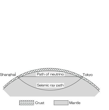
Figure 1: Schematic depiction of a hypothetical neutrino beam experiment.

Figure 2 shows the various density profiles under the hypothetical Tokyo-Shanghai path, taken from Model Crust 2.0. As shown in Fig. 2, the variation between the various density profiles is $\pm 4$ per cent in the depth range from 10–20 km and $\pm 7$ per cent in the depth range from 20–30 km. The variations in density are due to the differences in the physical properties of the various types of geological units, but can also be regarded as a crude indicator of the general level of uncertainty of the density. As, generally speaking, the amplitude of the Earth’s lateral hetereogeneity decreases with increasing depth, the variability of $\pm 7$ per cent in Fig. 2 can reasonably be regarded as as an upper bound on the uncertainty. Note that the density in the depth range 20–30 km in the rightmost column of Fig. 2 (3.35 g/cm³) is the value for the uppermost mantle, and is about 10 per cent higher than the density of the lowermost crust.

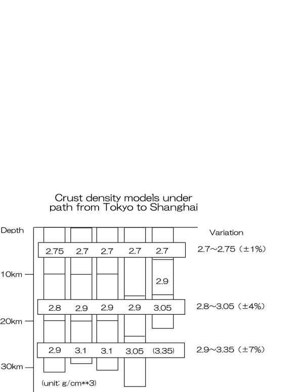
Figure 2: The various density profiles under the Tokyo-Shanghai path, from model Crust 2.0. Order from left to right is arbitrary.

4 Discussion

Neutrino beam physicists should be aware of the various uncertainties and limitations of present geophysical knowledge of the Earth’s density distribution, as discussed in this paper. The planning of neutrino beam experiments should include simulation of the data reduction process, including a propagation of error analysis, to study the effect of this uncertainty. Three possible scenarios can be envisioned. (1) The uncertainty of present density models poses no significant problems; (2) moderate reduction of the uncertainty, through more detailed analysis of existing data, is required: (3) significant reduction of this uncertainty, by conducting a large scale campaign of geophysical observations, is required. Obviously, scenario (1) would be most desirable, while scenario (3) would be discouraging. This issue should be resolved at an early stage of the planning of neutrino beam experiments.

References

Bullen, K., The Earth’s Density, Chapman & Hall (London, 1975).

Dziewonski, A. M., & Anderson, D. L., Preliminary reference Earth model, 1981, Phys. Earth Planet. Int., 25, 297-356.

Garnero, E. J., Heterogeneity of the lowermost mantle, 2000, Ann. Rev. Earth Planet. Sci., 28, 509-537.

Kennett, B. L. N., On the density distribution within the Earth, 1998, Geophys. J. Int., 132, 374-382.

Kennett, B. L. N., Engdahl, E. R., & Buland, R., Constraints on seismic velocities in the Earth from travel-times, 1995, Geophys. J. Int., 122, 108-124.

Lay, T., and T. C. Wallace, Modern Global Seismology, Academic (San Diego, 1995).

Mooney, W. D., Laske, G., & Masters, T. G., Crust 5.1: A global crustal model at $5^{o}\times 5^{o}$, 1998, J. Geophys. Res., 103, 727-747.

Nataf, H.-C., Seismic imaging of mantle plumes, 2000, Ann. Rev. Earth Planet. Sci., 28, 391-417.

Shearer, P. M., Introduction to Seismology, Cambridge U. Press (Cambridge, 1999).