We analyse a simple RPV extension of the MSSM, with bilinear R-parity violation in the soft terms and vevs, but not between the terms in the superpotential. The model gives two massive neutrinos, and can fit all constraints from neutrino data. We show analytically how to compute the lepton number violating Lagrangian parameters from neutrino masses and mixing angles. Conversely, we numerically vary the bilinear couplings as input parameters to determine the allowed ranges that are consistent with neutrino data. We briefly comment on the implications of our bounds for low energy LFV processes.

PACS number(s): 12.60.Jv, 14.60.Pq, 11.30.Fs

Neutrino Physics, Supersymmetric Standard Model, Solar and Atmospheric Neutrinos

I Introduction

The observed solar [1, 2] and atmospheric neutrino deficits [3, 4] can be explained by flavour-non-diagonal neutrino masses. The atmospheric neutrino anomaly is consistent with $\Delta m^{2}_{\rm atm}\sim(2-5)\times 10^{-3}~{}{\rm eV}^{2}$ (with $\sin^{2}2\theta_{\rm{atm}}>0.88$) [4]. The vacuum oscillation interpretation of solar neutrino data requires $\Delta m^{2}_{\rm solar}\sim 10^{-10}~{}{\rm eV}^{2}$, while the matter enhanced MSW solution prefers the range $\Delta m^{2}_{\rm solar}\sim(10^{-10}-10^{-4})~{}{\rm eV}^{2}$ [1, 2], see table I. In the standard three neutrino framework , which offers two independent mass differences, there are various mass hierarchies which can explain both solar and atmospheric results. These are summarised in table II. The oscillation explanation of the solar neutrino problem and the atmospheric neutrino anomaly requires two mixing angles and two hierarchical neutrino mass squared differences, namely $\Delta m^{2}_{{\mathrm{sun}}}\ll\Delta m^{2}_{{\mathrm{atm}}}$.

Experiment	$\Delta m^{2}$ (eV2)	$\sin^{2}2\theta$	$\tan^{2}\theta$
Atmospheric	$(2-5)\times 10^{-3}$	$0.88-1$	–
MSW-LMA	$(2-70)\times 10^{-5}$	$0.6\ -\ 1$	$(2-40)\times 10^{-1}$
MSW-SMA	$(0.4-1)\times 10^{-5}$	$10^{-3}\ -\ 10^{-2}$	$(1-30)\times 10^{-4}$
MSW-LOW	$4\times 10^{-10}-2\times 10^{-7}$	$0.7\ -\ 1$	$(1-80)\times 10^{-1}$
Vacuum	$(1-6)\times 10^{-10}$	$0.5\ -\ 1$	$(1-90)\times 10^{-1}$
Just-so	$(4-10)\times 10^{-12}$	$0.5\ -\ 1$	$(3-30)\times 10^{-1}$
Chooz	$>3\times 10^{-3}$	$\sin\theta<0.22$

TABLE I.: Allowed mass squared differences and mixing angles for MSW-LMA, MSW-SMA, MSW-LOW, Vacuum and Just-so stand for MSW large mixing angle, small mixing, and low, and for vacuum and just-so oscillation solutions, respectively. See e.g. [7]. We take the most conservative bounds.

Spectrum	Solar	Atmospheric
Hierarchical	$\Delta m_{12}^{2}$	$\Delta m_{13}^{2}$
Degenerate	$\Delta m_{23}^{2}\quad{\mathrm{or}}\quad\Delta m_{12}^{2}$	$\Delta m_{13}^{2}$
Pseudo-Dirac	$\Delta m_{23}^{2}\quad{\mathrm{or}}\quad\Delta m_{12}^{2}$	$\Delta m_{13}^{2}$

TABLE II.: Different possible regimes and corresponding mass squared difference.

We assume that the three neutrino masses $m_{i}$, $i=1,2,3$, satisfy $m_{1}<m_{2}<m_{3}$. As we will see, in our model we only have two non-zero neutrino masses thus our spectra can only be hierarchical or pseudo-Dirac, with $\Delta m_{\mathrm{a}tm}^{2}=\Delta m_{13}^{2}$ and $\Delta m_{\mathrm{s}olar}^{2}=\Delta m_{12}^{2},\Delta m_{23}^{2}$ respectively, see table II. The $3\times 3$ rotation matrix [8] (MNS) which rotates from neutrino flavour ($f$) to mass ($m$) eigenstates can be parametrised by three rotations: $V_{fm}=R_{23}(\theta_{23})R_{13}(\theta_{13})R_{12}(\theta_{12})$. We neglect the Majorana and Dirac phases, and write

$$V_{fm}=\left[\begin{array}[]{ccc}c_{12}c_{13}&c_{13}s_{12}&s_{13}\\ -c_{23}s_{12}-c_{12}s_{13}s_{23}&c_{12}c_{23}-s_{12}s_{13}s_{23}&c_{13}s_{23}\\ s_{23}s_{12}-c_{12}c_{23}s_{13}&-c_{12}s_{23}-c_{23}s_{12}s_{13}&c_{13}c_{23}\end{array}\right].$$ (1)

Massive neutrinos can be accomodated in the R-parity ($R_{p}$) violating Supersymmetric Standard Model [9, 10, 11, 12], where $R_{p}$ is defined as $(-1)^{3B+L+2S}$, and $B,L$ and $S$ are respectively the baryon number, lepton number and spin. $R_{p}$ is frequently imposed on the Supersymmetric SM to forbid renormalisable baryon and lepton number violating interactions. However, the phenomenological bounds on $B$ and/or $L$ violation [12] can be satisfied by imposing $B$ as a symmetry and allowing the lepton number violating couplings to be large enough to generate Majorana neutrino masses. We assume in this work that the baryon number violating couplings are absent, and concentrate on the “bilinear” lepton number violating interactions in the superpotential and soft terms. We neglect the trilinear R-parity violating (RPV) couplings that can appear in the superpotential.

Neutrino masses in RPV theories have been studied analytically for many years [10, 13], and recently numerically with more care [14, 15, 16]. The calculation of the neutrino masses to any given order can be performed by calculating the relevant self energy diagrams in the mass insertion approximation for the small RPV mass parameters. Alternatively, one can diagonalise the RPV mass matrices of particles which propagate in the loops. We use the mass insertion approximation, which allows us to identify analytically the contribution from the different parameters and thus use neutrino data to constrain the RPV couplings directly. Our purpose in this paper is to consider a simple model in which lepton number violation appears as a misalignment of the soft terms with respect to the superpotential. We then calculate the neutrino mass matrix in the mass insertion approximation.

Constraints on RPV parameters from neutrino masses and mixings are significant, as typically they provide the stronger bounds on the couplings than other low energy lepton-flavor violating (LFV) processes. In this paper we present two approaches in order to constrain the bilinear R-parity violating Lagrangian parameters. The first one is an analytic approach in which we obtain expressions for the two bilinear RPV parameters appearing in the Lagrangian in terms of neutrino masses and mixing angles. The second approach is a numerical one which follows that in ref [17, 18]. The bilinear parameters are varied as inputs and we use neutrino data to constrain the allowed ranges of these parameters. For that, since we only have ranges for the physically observed inputs, we constrain our parameter space (6 variables) by using the following inputs from neutrino data:

• $\Delta m^{2}_{\mathrm{atm}}$ and $\sin^{2}2\theta_{\mathrm{atm}}$,

• $\Delta m^{2}_{\mathrm{sun}}$ and $\sin^{2}2\theta_{\mathrm{sun}}$,

• $\sin\theta_{{\mathrm{Chooz}}}$.

Imposing these constraints implies an indirect restriction on the effective mass $m_{\mathrm{eff}}$ that enters the neutrinoless-double beta decay amplitude, i.e., $|m_{\mathrm{eff}}|\leq\sum_{i}m_{\nu_{i}}|V^{2}_{ei}|$. As we will show, we have checked in the different analyses we did of that the experimental bound [19] on $m_{\mathrm{eff}}$ is always satisfied.
The paper is organized as follows, in section II we present the model. Section III presents analytic and numerical results. Section IV discusses a model which generates neutrinos masses at tree-level and through loops considering only $R_{p}$-violating parameter contributions from the misalignment of the $\mu$ parameters and the vevs. In section V we discuss the implications of our results for low energy lepton flavour violating processes. We then present a summary of the paper.

II The Bilinear RPV Model

In a $R_{p}\!\!\!\!\!\!/~{}~{}$ supersymmetric model, the Higgs and the sleptons can mix (they have the same gauge quantum numbers), so the down-type Higgs and sleptons can be assembled in a vector $L_{J}=(H_{d},L_{i})$ with $J:4..1$. With this notation, the superpotential for the supersymmetric SM with $R_{p}$ violation can be written as

$$W=\mu^{J}{H}_{u}L_{J}+\frac{1}{2}\lambda^{JK\ell}L_{J}L_{K}E^{c}_{\ell}+\lambda^{{}^{\prime}Jpq}L_{J}Q_{p}D^{c}_{q}+h_{u}^{pq}{H}_{u}Q_{p}U^{c}_{q}~{}~{}.$$ (2)

The $R_{p}$ violating and conserving coupling constants have been assembled into vectors and matrices in $L_{J}$ space: we call the usual $\mu$ parameter $\mu_{4}$, and identify the usual $\epsilon_{i}=\mu_{i}$, $h_{e}^{jk}=\lambda^{4jk}$, and $h_{d}^{pq}=\lambda^{{}^{\prime}4pq}$. Lower case roman indices $i,j,k$ and $p,q$ are lepton and quark generation indices. We also include possible $R_{p}$ violating couplings among the soft SUSY breaking parameters, which can be written as

$$V_{soft} = \frac{\tilde{m}_{u}^{2}}{2}H_{u}^{\dagger}H_{u}+\frac{1}{2}L^{J\dagger}[\tilde{m}^{2}_{L}]_{JK}L^{K}+B^{J}H_{u}L_{J}$$ (4)

$$+A_{u}^{ps}H_{u}Q_{p}U^{c}_{s}+A^{{}^{\prime}Jps}L_{J}Q_{p}D^{c}_{s}+\frac{1}{2}A^{JKl}L_{J}L_{K}E^{c}_{l}+h.c.~{}~{}~{}.$$

Clearly field redefinitions of the $H_{d},L_{i}$ fields correspond to basis changes in $L_{J}$ space and consequently the Lagrangian parameters will be altered. Thus, whenever constraints are placed on the Lagrangian parameters the basis in which these are valid must be defined. Alternatively, we can construct basis-independent parametrisations of the couplings and constrain these. In this paper we take the second approach using the basis independent parameters $\delta_{\mu},\delta_{B}$, constructed in refs.[20, 21], which are defined in table III.
It is well known that this model can generate $\Delta L=2$ neutrino masses from tree-level and loop diagrams. There will be a non-zero neutrino mass at tree-level if $\mu_{I}\neq(\sqrt{\sum_{J}\mu_{J}^{2}}/\sqrt{\sum_{J}v_{J}^{2}})v_{I}$—that is if $(\mu_{4},\mu_{3},\mu_{2},\mu_{1})$ is not parallel with $(v_{4},v_{3},v_{2},v_{1})$ [9]. In the $v_{i}=\langle\tilde{\nu}_{i}\rangle=0$ basis, a neutrino $\nu_{3}$ acquires mass $m_{3}$ at tree level via a “seesaw”, with neutralinos playing the role of the heavy Majorana fermion, and the mass $\mu_{i}\nu_{i}\tilde{h}_{u}^{o}$ in the place of the “Dirac” mass, see figure 1.

FIG. 1.: Tree-level neutrino mass in the mass insertion approximation.

In the mass insertion approximation for $R_{p}\!\!\!\!\!\!/~{}~{}$ masses there are three types of loops that can contribute masses to the two neutrinos that are massless at tree level. There are the well-known loops involving trilinear $R_{p}\!\!\!\!\!\!/~{}~{}$ couplings $\lambda$ or $\lambda^{\prime}$ at both vertices. Then there is the Grossman-Haber diagram [11], figure 2, with gauge couplings at the vertices and $R_{p}\!\!\!\!\!\!/~{}~{}$ provided by mass insertions of the soft masses which mix the Higgses and the sleptons. Finally, there is figure 3, which has one gauge coupling and one trilinear/yukawa, and at least one unit of lepton number violation provided by a $R_{p}\!\!\!\!\!\!/~{}~{}$ mass insertion. The last two types of loops have frequently been neglected in analytic estimates of neutrino masses. In a previous work [20, 21], two of us showed that the analytic estimates in models with lepton number violating masses ($\equiv$ bilinear $R_{p}\!\!\!\!\!\!/~{}~{}$) suffer from two linked problems: confusion about the interaction eigenstate basis choice in the Lagrangian, and an incomplete set of one loop diagrams contributing to neutrino masses. “Basis independent” formulae for all the diagrams can be found in [21]. For a discussion of the construction of basis-independent invariants, see, e.g. [9, 20, 21, 22, 23, 24, 25].

R-parity violating models can be divided into classes based on which of the diagrams make significant contributions to the neutrino mass matrix $[m_{\nu}]_{ij}$ [20, 21]: in the first case, the loop diagrams with bilinear $R_{p}\!\!\!\!\!\!/~{}~{}$ are much smaller than the trilinear diagrams. In this case, $[m_{\nu}]_{ij}$ is due to the tree mass and the canonical $\lambda$ and $\lambda^{\prime}$ diagrams, and can have a large variety of patterns depending on the MSSM and $R_{p}\!\!\!\!\!\!/~{}~{}$ inputs. This case has recently been carefully studied in refs. [17, 18]. In the second case, the loops with bilinear $R_{p}\!\!\!\!\!\!/~{}~{}$ due to soft masses make significant contributions to $[m_{\nu}]_{ij}$, but the bilinears contributing at tree level$(\delta_{\mu}^{i})$ are negligible in the loops. This is the case we study in this section. To isolate the effect of the soft $R_{p}\!\!\!\!\!\!/~{}~{}$, we assume that the trilinears are negligible. The third possibility is that loops with lepton number violation from $\delta_{\mu}$ are important. Such loops can contribute $[m_{\nu}]_{ij}\sim\delta_{\mu}^{2}h_{\tau}^{2}m_{\tau}^{2}/(16\pi m_{SUSY})$, whereas the tree contribution is $m_{\nu}^{tree}\sim\delta_{\mu}^{2}m_{SUSY}$. This generates a very large hierarchy among neutrino masses, so this case is unlikely to be realised. We discuss this further in section IV.

$\begin{array}[]{||c|c||}\hline\cr\hline\cr&\\ \delta_{\mu}^{i}\equiv\frac{\vec{\mu}\cdot\lambda^{i}\cdot\vec{v}}{|\vec{\mu}|\sqrt{2}m_{e}^{i}}&\frac{\mu^{i}}{|\mu|}\\ &\\ \hline\cr&\\ \delta_{B}^{i}\equiv\frac{\vec{B}\cdot\lambda^{i}\cdot\vec{v}}{|\vec{B}|\sqrt{2}m_{e}^{i}}&\frac{B^{i}}{|B|}\\ &\\ \hline\cr&\\ \delta_{\lambda^{\prime}}^{ipq}\equiv\frac{\vec{\lambda}^{{}^{\prime}pq}\cdot\lambda^{i}\cdot\vec{v}}{\sqrt{2}m_{e}^{i}}&{\lambda}^{{}^{\prime}ipq}\\ &\\ \hline\cr&\\ \delta_{\lambda}^{ijk}\equiv\frac{\vec{v}\cdot\lambda^{i}\lambda^{k}\lambda^{j}\cdot\vec{v}}{2m_{e}^{i}m_{e}^{j}}&{\lambda}^{ijk}\\ &\\ \hline\cr\hline\cr\end{array}$

TABLE III.: The basis-independent invariants used to parametrise the bilinear $R_{p}\!\!\!\!\!\!/~{}~{}$ relevant for neutrino masses, together with their value in the $\langle\tilde{\nu}_{i}\rangle=0$ basis. They are zero if $R_{p}$ is conserved. (Note that these invariants have signs: for arbitrary vectors $\vec{a}$ and $\vec{b}$, $\vec{a}\cdot\lambda^{i}\cdot\vec{b}=-\vec{b}\cdot\lambda^{i}\cdot\vec{a}$).

FIG. 2.: The Grossman-Haber loop. The blobs indicate possible positions for $R_{p}\!\!\!\!\!\!/~{}~{}$ mass insertions. The misalignment between $\vec{\mu}$ and $\vec{v}$ allows a mass insertion on the lepton/higgsino lines (at points I, or VIII). The soft $R_{p}\!\!\!\!\!\!/~{}~{}$ masses appear as mass insertions at positions VI and IV on the scalar line.

FIG. 3.: Schematic representation of the charged loops with one gauge and a Yukawa coupling. These diagrams occur if gauginos mix with charged leptons—that is if $\delta_{\mu}\neq 0$. The blobs indicate possible positions for $R_{p}\!\!\!\!\!\!/~{}~{}$ interactions; each diagram contains two blobs. The $R_{p}\!\!\!\!\!\!/~{}~{}$ interactions can be trilinears (at VII) or mass insertions. The misalignment between $\vec{\mu}$ and $\vec{v}$ allows a mass insertion on the lepton/higgsino lines (at points I, III, or VIII), or on the scalar line at point $V$. The soft $R_{p}\!\!\!\!\!\!/~{}~{}$ masses can appear as a mass insertion at position IV.

We take in this section a model where $\delta_{B}^{i},\delta_{\mu}^{j}\neq 0$, and where $\delta_{\lambda},\delta_{\lambda^{\prime}}$ are negligible. Such a model could arise if the $R_{p}\!\!\!\!\!\!/~{}~{}$ is originated in the soft terms. It is interesting to consider because it shows the contribution of $\delta_{B}^{j}$ to $[m_{\nu}]_{ij}$, and allows us to set bounds on the $\delta_{B}^{j}$. We want to determine which values of $(\delta_{B}^{1},\delta_{B}^{2},\delta_{B}^{3})$ and $(\delta_{\mu}^{1},\delta_{\mu}^{2},\delta_{\mu}^{3})$ reproduce a neutrino mass matrix consistent with the data. We do this in two ways. First we assume that the neutrino masses and mixing angles are all known, and analytically solve for $\vec{\delta}_{\mu}$ and $\vec{\delta}_{B}$ as a function of the masses and mixing angles. This is tractable because the $\vec{\delta}_{\mu}$, $\vec{\delta}_{B}$ model only has two non-zero neutrino masses, so the algebra reduces to two dimensions.

Secondly, we start with $\vec{\delta}_{\mu}$ and $\vec{\delta}_{B}$ as inputs, varied over “sensible” ranges, and numerically determine whether the resulting neutrino mass matrix is consistent with observations using the inputs given above.

There are three relevant diagrams contributing to $[m_{\nu}]_{ij}$ in this model: the tree diagram of figure 1, and the Grossman-Haber diagram of figure 2 with $R_{p}\!\!\!\!\!\!/~{}~{}$ at points IV and VI, and with $R_{p}\!\!\!\!\!\!/~{}~{}$ at points I and VI. Exact formulae for these diagrams can be found in [21]. Our simplifying assumptions generate a neutrino mass matrix of the form

$$[m_{\nu}]_{ij}=m_{\mu}^{(0)}\hat{\delta}_{\mu}^{i}\hat{\delta}_{\mu}^{j}+m_{\mu B}^{(0)}(\hat{\delta}_{\mu}^{i}\hat{\delta}_{B}^{j}+\hat{\delta}_{B}^{i}\hat{\delta}_{\mu}^{j})+m_{B}^{(0)}\hat{\delta}_{B}^{i}\hat{\delta}_{B}^{j}$$ (5)

where

$$m_{\mu}^{(0)} = |\vec{\delta}_{\mu}|^{2}m_{SUSY}$$ (6)

$$m_{\mu B}^{(0)} = \frac{\alpha}{16\pi}|\vec{\delta}_{\mu}||\vec{\delta}_{B}|m_{SUSY}=\sqrt{\frac{\alpha}{16\pi}m_{\mu}^{(0)}m_{B}^{(0)}}$$ (7)

$$m_{B}^{(0)} = \frac{\alpha}{16\pi}|\vec{\delta}_{B}|^{2}m_{SUSY}$$ (8)

and $\alpha=\frac{g^{2}}{16\pi}$, $\hat{\delta}_{\mu}$ and $\hat{\delta}_{B}$ are unit vectors in $\{L^{i}\}$ space:

$$\hat{\delta}_{\mu}=\frac{1}{\sqrt{\sum_{i}(\delta_{\mu}^{i})^{2}}}(\delta_{\mu}^{e},\delta_{\mu}^{\mu},\delta_{\mu}^{\tau})~{}~{}~{}.$$ (9)

We have set all the unknown sparticle masses equal to $m_{SUSY}$ = 100 GeV, and neglected the mixing angles among MSSM particles. This is phenomenologically reasonable since superpartners have not been detected. Using the correct dependence on the MSSM parameters would have two effects: $m_{\mu B}^{(0)}$ would no longer be related to $m_{\mu}^{(0)}$ and $m_{B}^{(0)}$ as in eqn (7), and there could be additional (probably small) contributions to $[m_{\nu}]_{ij}$ with more complex index structure induced by spartner mass differences.

III Results

A $\vec{\delta}_{\mu}$ and $\vec{\delta}_{B}$ as a function of masses and mixing angles

In this section, we wish to go from the data to the Lagrangian parameters $\vec{\delta}_{\mu}$ and $\vec{\delta}_{B}$. We assume that the three neutrino masses (one of which is zero) and three mixing angles are all known exactly; from these six inputs we wish to analytically solve for the six parameters $\delta_{\mu}^{i}$ and $\delta_{B}^{i}$, $(i=1,3)$. The data do not fully determine $\vec{\delta}_{\mu}$ and $\vec{\delta}_{B}$, because these two vectors are not required to be orthogonal. An orthonormal basis would be $\hat{\delta}_{\mu}$ and $\hat{\delta}_{B_{\perp}}$ where

$$\hat{\delta}_{B_{\perp}}=\frac{1}{\sqrt{\sum_{i}(\delta_{B_{\perp}}^{i})^{2}}}(\delta_{B_{\perp}}^{e},\delta_{B_{\perp}}^{\mu},\delta_{B_{\perp}}^{\tau})~{}~{}~{},$$ (10)

and

$$\delta_{B_{\perp}}^{i}=\delta_{B}^{i}-(\delta_{B}\cdot\hat{\delta}_{\mu})\hat{\delta}_{\mu}^{i}~{}~{}~{}.$$ (11)

The parameters $\vec{\delta}_{\mu}$ and $\vec{\delta}_{B}$ can be expressed in terms of the two neutrino masses and the mixing angles, and one additional parameter which could be taken as the angle between $\vec{\delta}_{\mu}$ and $\vec{\delta}_{B}$ (which we will call $\rho$).

We first express the neutrino mass matrix $[m_{\nu}]_{ij}$ in terms of the orthonormal basis ($\hat{\delta}_{\mu}$, $\hat{\delta}_{B_{\perp}}$). Since $[m_{\nu}]_{ij}$ is a mass matrix in the two dimensional space spanned by $\vec{\delta}_{\mu}$ and $\vec{\delta}_{B}$, it has two non-zero eigenvalues and the problem reduces to two dimensional algebra. Secondly, we diagonalise $[m_{\nu}]_{ij}$, and compare the eigenvalues and eigenvectors to the observed masses and mixing angles. This allows us to determine $\vec{\delta}_{\mu}$ and $\vec{\delta}_{B}$ as a function of the masses and mixing angles, and one free parameter. The free parameter arises because $\vec{\delta}_{\mu}$ and $\vec{\delta}_{B}$ are not orthogonal, so what fraction of the heavier neutrino mass is due to $\vec{\delta}_{B}$ is a free parameter.

In the ($\hat{\delta}_{\mu}$, $\hat{\delta}_{B_{\perp}}$) basis, $[m_{\nu}]_{ij}$ can be written

$$[m_{\nu}]_{ij} = (m_{\mu}^{(0)}+2m_{\mu B}^{(0)}\cos\rho+m_{B}^{(0)}\cos^{2}\rho)\hat{\delta}_{\mu}^{i}\hat{\delta}_{\mu}^{j}$$ (13)

$$+(m_{\mu B}^{(0)}\sin\rho+m_{B}^{(0)}\sin\rho\cos\rho)(\hat{\delta}_{\mu}^{i}\hat{\delta}_{B_{\perp}}^{j}+\hat{\delta}_{B_{\perp}}^{i}\hat{\delta}_{\mu}^{j})+m_{B}^{(0)}\sin^{2}\rho\hat{\delta}_{B_{\perp}}^{i}\hat{\delta}_{B_{\perp}}^{j}$$

$$\equiv m_{\mu}\hat{\delta}_{\mu}^{i}\hat{\delta}_{\mu}^{j}+m_{\mu B}(\hat{\delta}_{\mu}^{i}\hat{\delta}_{B_{\perp}}^{j}+\hat{\delta}_{B_{\perp}}^{i}\hat{\delta}_{\mu}^{j})+m_{B}\hat{\delta}_{B_{\perp}}^{i}\hat{\delta}_{B_{\perp}}^{j}$$ (14)

where $\rho$ is the angle between $\hat{\delta}_{\mu}$ and $\hat{\delta}_{B}$ : $\cos\rho=\hat{\delta}_{\mu}\cdot\hat{\delta}_{B}$. The matrix $[m_{\nu}]_{ij}$ has two non-zero eigenvalues, so the neutrino mass spectrum is either hierarchical with $\Delta m^{2}_{atm}=m_{3}^{2}$ and $\Delta m^{2}_{sol}=m_{2}^{2}$, or pseudo-Dirac, with $\Delta m^{2}_{atm}=m_{3}^{2},m_{2}^{2}$ and $\Delta m^{2}_{sol}=m_{3}^{2}-m_{2}^{2}$. The eigenvectors are the last two columns of $V_{fm}$ in eq. (1), and lie in the 2-d sub-space spanned by $(\delta_{B}^{1},\delta_{B}^{2},\delta_{B}^{3})$ and $(\delta_{\mu}^{1},\delta_{\mu}^{2},\delta_{\mu}^{3})$.

We can now determine $(\delta_{B}^{1},\delta_{B}^{2},\delta_{B}^{3})$ and $(\delta_{\mu}^{1},\delta_{\mu}^{2},\delta_{\mu}^{3})$ as a function of the neutrino masses and mixing angles, and the angle $\gamma$ between $(\delta_{\mu}^{1},\delta_{\mu}^{2},\delta_{\mu}^{3})$ and $(V_{13},V_{23},V_{33})$. We solve for the angle $\rho$ (between $\vec{\delta}_{B}$ and $\vec{\delta}_{\mu}$) as a function of $\gamma$ in equation (19).

In the mass eigenstate basis spanned by $V_{f2}$ and $V_{f3}$ ($f:1..3)$, the neutrino mass matrix is

$$\left[\begin{array}[]{cc}m_{2}&0\\ 0&m_{3}\end{array}\right].$$ (15)

Suppose that $(\delta_{\mu}^{1},\delta_{\mu}^{2},\delta_{\mu}^{3})$ is rotated by an angle $\gamma$ with respect to $(V_{13},V_{23},V_{33})$, so that the mass matrix (15) is

$$\left[\begin{array}[]{cc}\cos^{2}\gamma m_{2}+\sin^{2}\gamma m_{3}&\cos\gamma\sin\gamma(m_{2}-m_{3})\\ \cos\gamma\sin\gamma(m_{2}-m_{3})&\cos^{2}\gamma m_{3}+\sin^{2}\gamma m_{2}\end{array}\right]=\left[\begin{array}[]{cc}m_{B}&m_{\mu B}\\ m_{\mu B}&m_{\mu}\end{array}\right],$$ (16)

in the basis of $(\delta_{\mu}^{1},\delta_{\mu}^{2},\delta_{\mu}^{3})$ and $(\delta_{B_{\perp}}^{1},\delta_{B_{\perp}}^{2},\delta_{B_{\perp}}^{3})$. By comparing eqn (16) to eqn (14), we find

$$m_{B}^{(0)}\sin^{2}\rho\equiv\frac{\alpha}{16\pi}|\delta_{B}|^{2}m_{SUSY}\sin^{2}\rho=(\cos^{2}\gamma m_{2}+\sin^{2}\gamma m_{3})$$ (17)

$$m_{\mu}^{(0)}\left(1-\frac{\alpha}{16\pi}\right)\equiv|\delta_{\mu}|^{2}m_{SUSY}\left(1-\frac{\alpha}{16\pi}\right)=\frac{m_{2}m_{3}}{\cos^{2}\gamma m_{2}+\sin^{2}\gamma m_{3}}$$ (18)

$$\cot\rho=\frac{\cos\gamma\sin\gamma(m_{2}-m_{3})}{\cos^{2}\gamma m_{2}+\sin^{2}\gamma m_{3}}-\sqrt{\frac{\alpha}{16\pi}\frac{m_{2}m_{3}}{(\cos^{2}\gamma m_{2}+\sin^{2}\gamma m_{3})^{2}}}$$ (19)

$$\frac{1}{|\delta_{\mu}|}\delta_{\mu}^{f}=\cos\gamma V_{f3}+\sin\gamma V_{f2}$$ (20)

$$\frac{1}{|\delta_{B_{\perp}}|}\delta_{B_{\perp}}^{f}=-\sin\gamma V_{f3}+\cos\gamma V_{f2}.$$ (21)

We can now determine the values of $(\delta_{\mu}^{1},\delta_{\mu}^{2},\delta_{\mu}^{3})$ and $(\delta_{B}^{1},\delta_{B}^{2},\delta_{B}^{3})$ corresponding to atmospheric and different solar solutions.

We first compute values of $|\delta_{\mu}|$ and $|\delta_{B}|$ that give solar and atmospheric neutrino masses.
To get degenerate masses $m_{2}\sim m_{3}\sim\sqrt{\Delta m^{2}_{atm}}$, the angle $\rho$ between $\vec{\delta}_{B}$ and $\vec{\delta}_{\mu}$ must be of order $\pm\pi/2$. So $\vec{\delta}_{B}$ must be approximately orthogonal to $\vec{\delta}_{\mu}$, and $\frac{\alpha}{16\pi}|{\delta}_{B}|^{2}\simeq|{\delta}_{\mu}|^{2}\simeq\sqrt{\Delta m^{2}_{atm}}/m_{SUSY}$. This seems unnatural and fine-tuned, so we do not pursue this possibility.
For the case of hierarchical neutrino masses, we plot in figure 4 the allowed values of $|\delta_{\mu}|$ and $|\delta_{B}|$ corresponding to combined constraints from Chooz and atmospheric (SuperK) results and three of the solar solutions. The allowed parameter space corresponds to the space contained between the lines in figure 4. The shortest pair of lines corresponds to the LMA MSW solution, the middle lines to the SMA solution and the longest pair of lines to the Vacuum solution. We obtain these two lines by varying the angle $\gamma$ for the maximum and minimum allowed values of the masses $m_{2}$ and $m_{3}$, as given in table I. In this plot (fig.4), the left [bottom] end of the allowed parameter space corresponds to $m_{3}$ induced by ${\delta}_{B}$ [${\delta}_{\mu}$].

FIG. 4.: Allowed region in parameter space for various solar oscillation solutions combined with the atmospheric and Chooz constraints. The allowed region is between the lines; the longest pair of lines correspond to the vacuum solar solution, and the shortest [middle length] lines to the LMA [SMA] MSW solution.

It was pointed out in [16] that their MSUGRA bilinear model was effectively controlled by two vectors, $\vec{\delta}_{\mu}$ and the misalignment between $\mu$ and the trilinears ($\equiv\delta_{\lambda}$). The parametrisation of equations (17) to (21) should therefore approximately describe the results of [16], replacing $\vec{\delta}_{B}$ by $\vec{\delta}_{\lambda}$. Their heavy neutrino mass $m_{3}$ is induced by the tree diagram of figure 1, so the angle $\gamma$ (between the eigenvector corresponding to $m_{3}$ and $\vec{\delta}_{\mu}$) is small. It is easy to see from equation (20) that the atmospheric mixing angle is therefore controlled by the relative size of $\delta_{\mu}^{\mu}$ and $\delta_{\mu}^{\tau}$, as was indeed found by [16]. We see from equation (21) that the solar mixing angles are determined from the relative size of the elements of $\vec{\delta}_{B_{\perp}}$, rather than from the elements of $\vec{\delta}_{B}$. This means that the solar angle will sometimes show a correlation with the elements of $\vec{\delta}_{B}$, specifically if $\vec{\delta}_{B}$ is approximately perpendicular to $\vec{\delta}_{\mu}$. This agrees with the results of [16].

The Chooz results require $V_{e3}=\cos\gamma\hat{\delta}_{\mu}^{e}-\sin\gamma\hat{\delta}_{B_{\perp}}^{e}\mathrel{\hbox to0.0pt{\raise 2.15277pt\hbox{$<$}\hss}{\lower 2.15277pt\hbox{$\sim$}}}.1$. For large angle solar solutions (LMA), $V_{e2}\sim 1/\sqrt{2}$, so $\hat{\delta}_{\mu}^{e}\simeq\frac{1}{\sqrt{2}}\sin\gamma$, and $\hat{\delta}_{B_{\perp}}^{e}\simeq\frac{1}{\sqrt{2}}\cos\gamma$, and $V_{e3}$ is small due to a cancellation between $\hat{\delta}_{\mu}^{e}$ and $\hat{\delta}_{B_{\perp}}^{e}$. For small angle solar solutions, both $\hat{\delta}_{\mu}^{e}$ and $\hat{\delta}_{B_{\perp}}^{e}$ may be small. This scenario has cosmological attractions, because it would allow a baryon asymmetry produced before the electroweak phase transition to survive. Baryon + lepton number violating processes are in thermal equilibrium before the electroweak phase transition, so a primordial asymmetry must be stored in a conserved quantum number (which could be one of the $B/3-L_{i})$ to survive. For $B/3-L_{e}$ to be effectively conserved before the phase transition, we need [27] $(B_{4}{\mu}^{e}-\mu_{4}{B}^{e})\mathrel{\hbox to0.0pt{\raise 2.15277pt\hbox{$<$}\hss}{\lower 2.15277pt\hbox{$\sim$}}}2\times 10^{-7}|\mu||B|/\tan\beta$. For $\delta_{\mu}\sim 10^{-6}$, $\delta_{B}\sim 10^{-4}$, as could generate the atmospheric and SMA solar masses, this is satisfied for $\hat{\delta}_{\mu}^{e}\mathrel{\hbox to0.0pt{\raise 2.15277pt\hbox{$<$}\hss}{\lower 2.15277pt\hbox{$\sim$}}}.1$ or $\hat{\delta}_{B}^{e}\mathrel{\hbox to0.0pt{\raise 2.15277pt\hbox{$<$}\hss}{\lower 2.15277pt\hbox{$\sim$}}}2\times 10^{-3}$.

In the case of a hierarchical spectrum, then only for very small values of the angle $\gamma$ do we find that $\cos^{2}\gamma m_{2}\sim\sin^{2}\gamma m_{3}$. In this case $|\delta_{\mu}|$ will generate the neutrino with a mass $m_{3}\rightarrow\sqrt{\Delta m_{atm}^{2}}$ and $|\delta_{B}|$ will generate the neutrino with a mass $m_{2}\rightarrow\sqrt{\Delta m_{solar}^{2}}$. For all other values of $\gamma$ then $|\delta_{B}|\rightarrow\sqrt{\Delta m_{atm}^{2}}$ and $|\delta_{\mu}|\rightarrow\sqrt{\Delta m_{solar}^{2}}$. That is, the loop is giving the largest contribution to the neutrino masses. So the “measure” on parameter space determined by the angle $\gamma$ does not correspond to natural theoretical expectations. For large values of $\gamma$ the atmospheric mixing angle is now controlled by the relative size of $\delta_{B_{\perp}}^{\mu}$ and $\delta_{B_{\perp}}^{\tau}$.

B Masses and mixing angles from $\vec{\delta}_{\mu}$ and $\vec{\delta}_{B}$

In this subsection we present numerical results of our scan of parameter space varying the inputs parameters in the range of $|\delta_{\mu}|<10^{-6}$ and $|\delta{{}_{B}}|<4.10^{-5}$. This scan allows us to consider the case when tree contributions are larger, of the same order or smaller than the loop contributions. 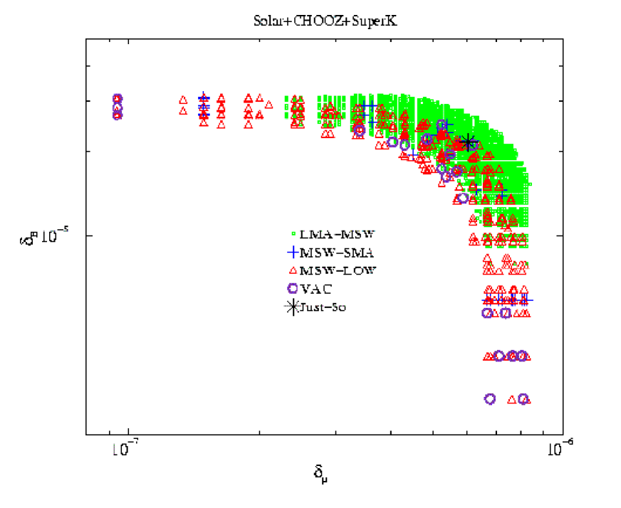We present in figure 5 the allowed region in parameter space in the $|\delta_{B}|$ vs $|\delta_{\mu}|$ plane, these results are in agreement with the ones obtained in ref. [21]. The different points displayed correspond to combined constraints from Chooz+SuperK atmospheric data and one of the solar solutions. As expected, figures 5 and 4 are quite similar.

FIG. 5.: We present the available region in parameter space for a combined fit using Chooz, atmospheric and one of the solar oscillations solutions.

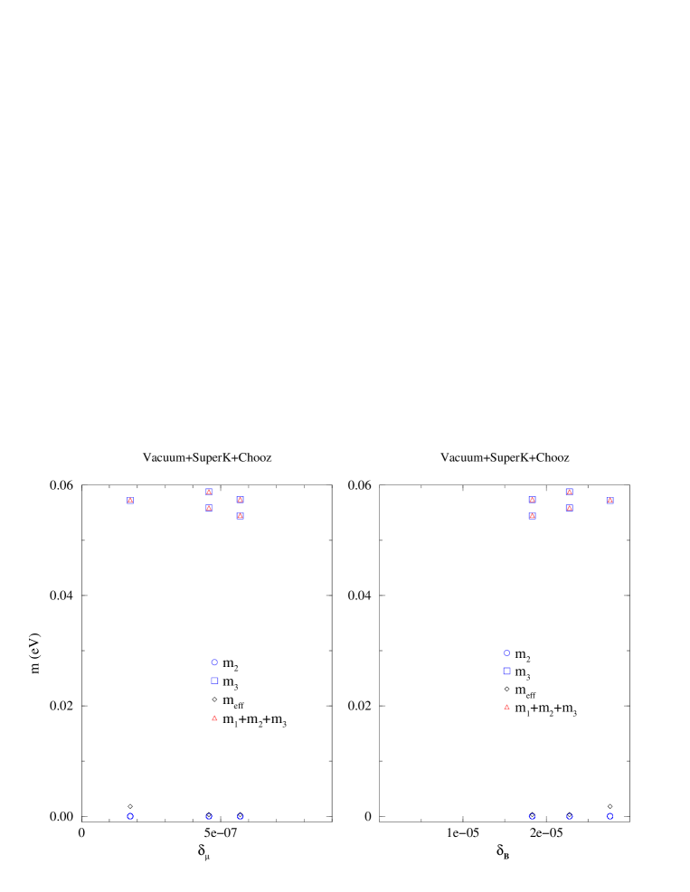
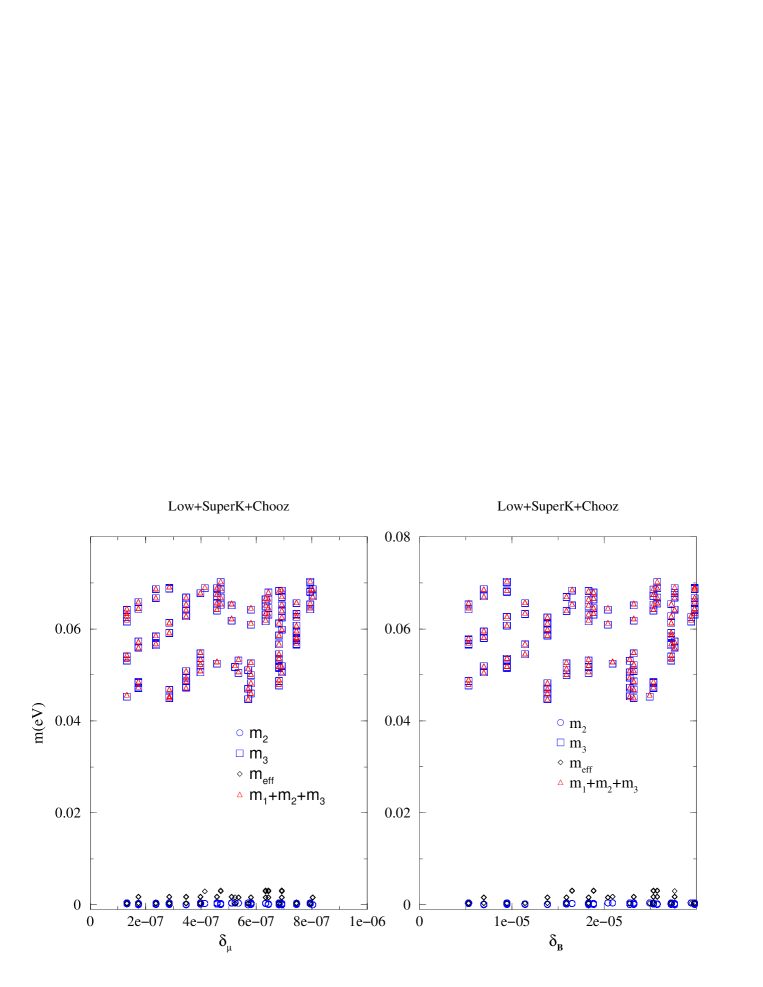
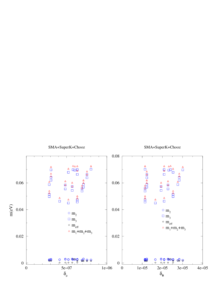
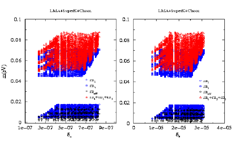
In order to study the spectrum for each of the possible combined solutions we give samples of the different mass spectra for different values of the input parameters $\vec{\delta}_{\mu}$ and $\vec{\delta}_{B}$. For illustration, in figures 6,7, 8 and 9 we present the obtained spectra for the combined constraint of Chooz and the atmospheric SuperK data with one of the solar solutions as functions of $|\delta_{\mu}|$ and $|\delta_{B}|$ . We also plot $m_{eff}$ and $\sum_{i}m_{i}$ and we see that the bounds from neutrinoless double beta decay [19] and the cosmological constraint $\sum_{i}m_{i}\mathrel{\vbox{\hbox{$<$}\nointerlineskip\hbox{$\sim$}}}$few eV are respectively fulfilled. From these plots one can read that the scan shows us only hierarchical spectra for all combined constraints.

FIG. 6.: The mass spectrum is represented together with $m_{\mathrm{eff}}$ and the sum of the eigenvalues in the case of a combined fit with Chooz, Vacuum solar solution and atmospheric SuperK constraints.

FIG. 7.: The mass spectrum together with the effective mass $m_{\mathrm{eff}}$ and the sum of the eigenvalues are represented for a combined fit with Chooz, Superk and MSW-LOW oscillation solutions.

FIG. 8.: The mass spectrum together with the effective mass $m_{\mathrm{eff}}$ and the sum of the eigenvalues are represented in the case of a combined fit with Chooz, Superk atmospheric and MSW-SMA oscillation solutions.

FIG. 9.: The mass spectrum together with the effective mass $m_{\mathrm{eff}}$ and the sum of the eigenvalues are represented for a combined fit with Chooz, Superk atmospheric and MSW-LMA constraints.

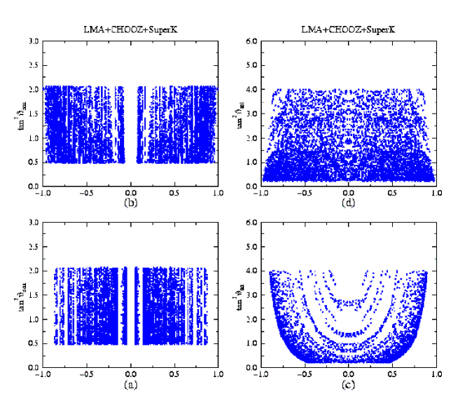
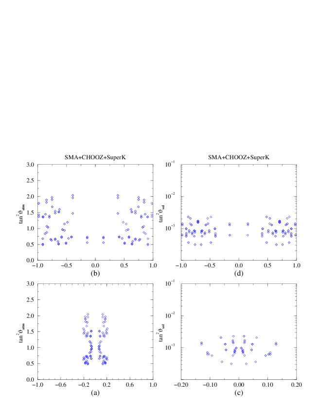
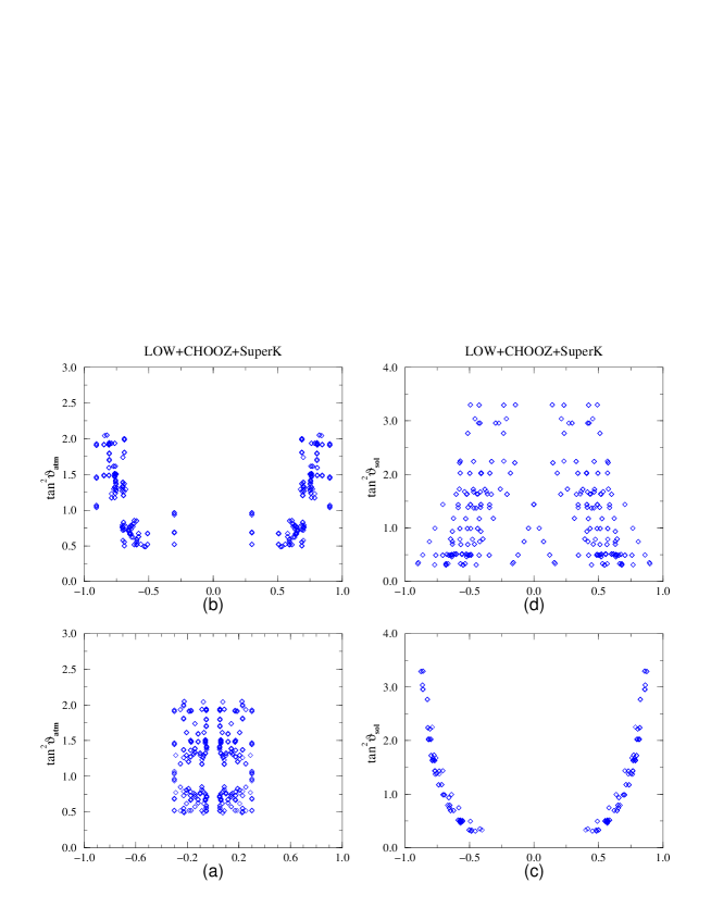
In figures 10, 11, 12 and 13 we plot the different solar and atmospheric mixing angles as functions of the R-parity violating parameters ${|\delta_{\mu}^{1,2}|\over|\delta_{\mu}|}$ and ${|\delta_{B_{\perp}}^{1,2}|\over|\delta_{B_{\perp}}|}$. The allowed ranges for the RPV parameters agree with the estimates of equations (20) and (21).

In general, the observed discreteness in all our plots is in part due to the step taken in our scan of parameter space and we note that the dependence on a single parameter is complicated since many solutions can be found for the same input value. Also the same value of the physical parameter involved can correspond to different values of the inputs.

FIG. 10.: The allowed atmospheric and solar angles for a combined fit of MSW-LMA, Chooz and SuperK atmospheric data. The atmospheric (solar) angle is plotted as a function of ${|\hat{\delta}_{\mu}^{1}|}$ and ${|\hat{\delta}_{\mu}^{2}|}$ (${|\hat{\delta}_{B_{\perp}}^{1}|}$ and ${|\hat{\delta}_{B_{\perp}}^{2}|}$) in (a) and (b) (in (c) and (d)) respectively.

FIG. 11.: The allowed atmospheric and solar angles for a combined fit of MSW-SMA, Chooz and SuperK atmospheric data. The atmospheric (solar) angle is plotted as a function of ${|\hat{\delta}_{\mu}^{1}|}$ and ${|\hat{\delta}_{\mu}^{2}|}$ (${|\hat{\delta}_{B_{\perp}}^{1}|}$ and ${|\hat{\delta}_{B_{\perp}}^{2}|}$) in (a) and (b) (in (c) and (d)) respectively.

FIG. 12.: The allowed atmospheric and solar angles for a combined fit of MSW-LOW, Chooz and SuperK atmospheric constraints. The atmospheric (solar) angle is plotted as a function of ${|\hat{\delta}_{\mu}^{1}|}$ and ${|\hat{\delta}_{\mu}^{2}|}$ (${|\hat{\delta}_{B_{\perp}}^{1}|}$ and ${|\hat{\delta}_{B_{\perp}}^{2}|}$) in (a) and (b) (in (c) and (d)) respectively.

FIG. 13.: The allowed atmospheric and solar angles for a combined fit of Vacuum, Chooz and SuperK atmospheric solutions.The atmospheric (solar) angle is plotted as a function of ${|\hat{\delta}_{\mu}^{1}|}$ and ${|\hat{\delta}_{\mu}^{2}|}$ (${|\hat{\delta}_{B_{\perp}}^{1}|}$ and ${|\hat{\delta}_{B_{\perp}}^{2}|}$) in (a) and (b) (in (c) and (d)) respectively.

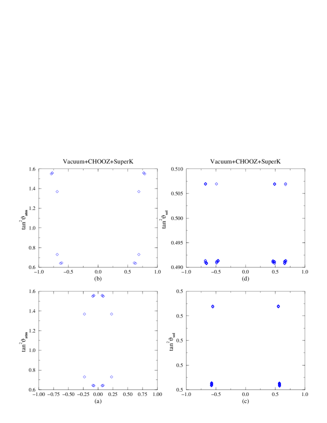
IV Model with only $\delta_{\mu}$

In this section, we show that a realistic neutrino mass matrix cannot be generated in an RPV model where only the invariant $\vec{\delta}_{\mu}$ is non-zero. This toy model is interesting because it allows us to study whether the $O(|\delta_{\mu}|^{2})$ loop contributions to $[m_{\nu}]_{ij}$ need to be taken into account. We assume that the only non-zero invariant is $\vec{\delta}_{\mu}$, and ask whether we can generate $m_{2}$ from the $\delta_{\mu}$ loops of figure 3 if $m_{3}$ is due to the tree level diagram of figure 1. The answer is no, even for large $\tan\beta$, because the loop mass is necessarily small (of order the vacuum or just-so masses), and the solar mixing angle is also small.

The analysis of this section is quite relevant as this type of model has been constrained using other low energy LFV processes, as in [29]. However, as mentioned in the introduction, typically neutrino data will put tighter constraints on the RPV parameters and as we have seen it is not possible to accomodate all neutrino data simultaneously.

We take

$$|\vec{\delta}_{\mu}|\sim\frac{[\Delta m^{2}_{atm}]^{1/4}}{m_{SUSY}}$$ (22)

and $\delta_{\mu}^{\mu}\sim\delta_{\mu}^{\tau}\gg\delta_{\mu}^{e}$ so that the heaviest neutrino mass $m_{3}$ explains the atmospheric neutrino anomaly and is consistent with Chooz. The solar neutrino mass will come from the “see-saw-type” loops of figure 3, with one $\delta_{\mu}$ mass insertion on an external leg.

The diagrams of figure 3 can have R-parity violating mass insertions at (I,V), (I,III) or (III,VIII). The potentially largest is (I,V) (see [21] for exact formulae), because it is proportional to $\tan\beta$:

$$(I,V)\sim g\delta_{\mu}^{i}\delta_{\mu}^{j}\tan\beta\frac{m_{e_{j}}^{2}}{16\pi^{2}m_{SUSY}}~{}~{}~{}~{}.$$ (23)

We refer to this as “see-saw-type” because it is a mass between the neutrino $\nu_{3}$ who acquired mass at tree level, and the massless-at-tree-level neutrinos $\nu_{2}$ and $\nu_{1}$. Neglecting the muon and electron masses with respect to the tau mass, equation (23) is a mass between $\nu_{3}$ and $\nu_{\tau}$. The largest see-saw mass it could induce for $\nu_{2}$ would arise if $\nu_{2}\sim\nu_{\tau}$, and is of order

$$m_{2}\mathrel{\vbox{\hbox{$<$}\nointerlineskip\hbox{$\sim$}}}m_{\nu}^{tree}\left(\frac{\tan\beta h_{\tau}^{2}}{8\pi^{2}}\right)^{2}~{}~{}~{}.$$ (24)

This could generate $m_{2}\sim 10^{-5}m_{\nu}^{tree}$ for $\tan\beta\sim 50$. So if all free parameters are stretched, it might just be possible to get a “see-saw” loop mass of order the Vacuum or JUST SO solar neutrino masses.

The neutrino which gets a loop mass will only have a very small $\nu_{e}$ component, so will not have the large mixing angle required for the Vacuum and JUST SO solar solutions. However, recall that we choose $\delta_{\mu}^{\tau}\sim\delta_{\mu}^{\mu}\gg\delta_{\mu}^{e}$, so that the tree level mass explains the atmospheric neutrino anomaly and agrees with Chooz. The loops mix $\nu_{3}$ with $\nu_{\tau}$, so the second massive neutrino will be composed largely of $\nu_{\tau}$ and $\nu_{\mu}$, and the massless neutrino will be mostly $\nu_{e}$. An $R_{p}$ violating model with $\delta_{\mu}\neq 0$ and all the other invariants zero therefore can not explain observed neutrino data.

V Effects on low energy LFV processes

It is also of interest to comment on the effects of the allowed values for the different $\delta_{B}^{i}$, $\delta_{\mu}^{i}$ from neutrino masses and mixings on low energy lepton flavour violating processes. In this model there can be tree level contributions from the RPV parameters to some of the $\Delta L=0$ processes. We can estimate the contributions to processes like $\mu\rightarrow e\gamma$, $\mu\rightarrow eee$ $\mu-e$ conversion in nuclei, and other LFV processes at low energy.

In general the branching ratios for these processes will be proportional to

$$\left({\delta_{\mu}^{i}\delta_{\mu}^{j}\over G_{f}m_{susy}^{2}}\right)^{2},\hskip 28.45274pt\left({\delta_{B}^{i}\delta_{B}^{j}\over G_{f}m_{susy}^{2}}\right)^{2},\hskip 28.45274pt\left({\delta_{\mu}^{i}\delta_{B}^{j}\over G_{f}m_{susy}^{2}}\right)^{2}.$$ (25)

Thus it is trivial to see using simple estimates that the branching ratios of low energy lepton flavour violating processes will automatically be suppressed given the constraints from neutrino data. The obtained branching ratios are well below current and anticipated experimental values.

Our simple model for generating neutrino masses and mixings correlates the ratios of branching ratios of different LFV low energy processes. The exact values of these correlations will depend on the combined constraint of solar, atmospheric and Chooz experiments which is used.

A generic consequence of this model is that the lightest supersymmetric particle (LSP) will decay. The details of this analysis will be presented elsewhere.

VI SUMMARY

In this paper, we studied a minimal model of bilinear $R_{p}$ violation which is consistent with the atmospheric and solar neutrino anomalies. In the “basis-independent” formalism in which we work, the model has $\vec{\delta}_{\mu}\neq\vec{\delta}_{B}\neq 0$, and all other invariants zero . In the basis where there are no $R_{p}\!\!\!\!\!\!/~{}~{}$ trilinears, this model has R-parity violating $B_{i}H_{u}L^{i}$ masses and sneutrino vevs. Such a model could arise if the superpotential was $R_{p}$ conserving, but R-parity violation was introduced through the soft terms.

In the limit where we neglect MSSM mixing angles and set all spartner masses to a common scale $m_{SUSY}$, the neutrino mass matrix is controlled by the 6 parameters $\delta^{i}_{\mu},\delta^{i}_{B}$ (i: 1..3). There are two massive neutrinos. If we make the simplifying assumption that we know the neutrino masses and the mixing matrix (MNS) exactly, we can solve for $\vec{\delta}_{\mu}$ and $\vec{\delta}_{B}$ as a function of one additional parameter, which can be taken as the angle between $\vec{\delta}_{\mu}$ and $\vec{\delta}_{B}$. We plot the allowed values of $|\vec{\delta}_{\mu}|$ versus $|\vec{\delta}_{B}|$ for different solar solutions in figure 4. See also figure 5. This gives some idea of the weak-scale $R_{p}\!\!\!\!\!\!/~{}~{}$ Lagrangian mass terms which can induce a phenomenologically correct neutrino sector. In reality however, we do not know the neutrino masses or the MNS matrix elements exactly, so we numerically vary the six inputs parameters, and find ranges where the neutrino masses and MNS matrix elements are consistent with combined fits of SuperK, Chooz and solar data.

This model differs from usual models of bilinear $R_{p}\!\!\!\!\!\!/~{}~{}$ in that it has different loop diagrams. $\vec{\delta}_{B}$ generates a loop contribution to the neutrino mass matrix of order $g^{2}|\vec{\delta}_{B}|^{2}m_{SUSY}$ via the Grossman-Haber diagram of figure 2. This diagram has frequently been overlooked in the literature. If $\vec{\delta}_{\mu}\propto\vec{\delta}_{B}$, then this is a loop correction to the tree mass and so its not useful to generate another neutrino mass. However we treat $\vec{\delta}_{\mu}$ and $\vec{\delta}_{B}$ as phenomenological weak-scale inputs, and allow them to vary independently. The Grossman-Haber diagram is therefore the source of our loop neutrino masses. This is in contrast to a MSUGRA bilinear model, where $\mu$ is misaligned at the GUT scale with respect to the trilinears, and the loop diagrams are proportional to trilinear couplings squared. The trilinear diagrams are more important than the Grossman-Haber diagram in MSUGRA models, because renormalisation group running makes the latter a loop correction to the tree level mass ($\vec{\delta}_{\mu}\sim\vec{\delta}_{B}$).

The simplicity of this $\vec{\delta}_{\mu}-\vec{\delta}_{B}$ model is attractive: neutrino oscillations can be explained with six additional parameters (and all of the MSSM!). This is in contrast to most models with trilinear R-parity violation, where a multitude of couplings contribute to the neutrino masses. The phenomenology of this model is quite different from other RPV violating models with respect to the scalar sector of the theory. For neutrino masses $m_{3}=\sqrt{\Delta m^{2}_{atm}}$ and $m_{2}=\sqrt{\Delta m^{2}_{sol}}$ and a given MNS matrix, the $R_{p}\!\!\!\!\!\!/~{}~{}$ mass terms $B_{i}$ and $\mu_{i}$ in the Lagrangian are determined as a function of one free parameter, which is the angle $\gamma$ in equations (17) to (21). This parametrisation can describe more general models of bilinear $R_{p}\!\!\!\!\!\!/~{}~{}$ under certain circumstances, as was discussed in section III A. We have also shown that combined solutions of SuperK, Chooz and all possible solar oscillations solutions can be obtained.

REFERENCES

- [1] Q.R. Ahmed et al.,, “Measurement of charged current interactions produced by solar neutrinos at the Sudbury Neutrino Observatory”.
- [2] B.T. Cleveland et al., Nucl. Phys. B (Proc. Suppl.) 38, 47 (1995); Kamiokande Collaboration, Y. Fukuda et al., Phys. Rev. Lett. 77, 1683 (1996); GALLEX Collaboration, W. Hampel et al., Phys. Lett. B 388, 384 (1996); SAGE Collaboration, J.N. Abdurashitov et al., Phys. Rev. Lett. 77, 4708 (1996); J.N. Bahcall, M.H. Pinsonneault, Rev. Mod. Phys. 67, 781 (1995).
- [3] R. Becker-Szendy et al., IMB Collaboration, Nucl. Phys. B (Proc. Suppl.) 38 (1995) 331. W.W.M. Allison et al. Soudan-2 Collaboration, Phys. Lett. B391 (1997) 491, Phys. Lett. B449 (1999) 137. Y. Fukuda et al., Kamiokande Collaboration, Phys. Lett. B 335 (1994) 237. R. Davis et al., Phys.Rev.Lett. 21 (1968) 1205; B.T. Cleveland et al., Astrophys. J. 496 (1998) 505. W. Hampel et al., Phys. Lett. B 388 (1996) 384. D.N. Abdurashitov et al., Phys. Rev. Lett. B 77 (1996) 4708; astro-ph/9907131. K. S. Hirata et al., Kamiokande Collaboration, Phys. Rev. Lett. 77 (1996) 1683.
- [4] Super-Kamiokande Collaboration, Y. Fukuda et al., Phys. Rev. Lett. 81, 1562 (1998), Phys. Rev. Lett. 85, 3999 (2000).
- [5] LSND Collaboration, C. Athanassopoulos et al., Phys. Rev. Lett. 75, 2650 (1995); ibid. 77, 3082 (1996); ibid. 81, 1774 (1998); Phys. Rev. C 58, 2489 (1998).
- [6] A.O. Bazarkoet al., Nucl. Phys. Proc. Suppl. 91, 210 (2000) .
- [7] J. N. Bahcall, M.C. Conzalez-Garcia, C. Pena-Garay, hep-ph/0106258; P.I. Krastev and A. Yu. Smirnov, hep-ph/0108177; G.L. Fogli et al, hep-ph/0106247.
- [8] Z. Maki, M. Nakagawa and S. Sakata, Prog. Theor. Phys. 28 (1962) 870.
- [9] H.P. Nilles and N. Polonsky, Nucl. Phys. B499 (1997) 33. T. Banks, Y. Grossman, E. Nardi and Y. Nir, Phys. Rev. D52 (1995) 5319. F.M. Borzumati, Y. Grossman, E. Nardi and Y. Nir, Phys.Lett. B384 (1996) 123. E.Nardi, Phys. Rev. D55 (1997) 5772.
- [10] L. Hall and M. Suzuki. Nucl. Phys., B231:419, 1984.
- [11] Y. Grossman and H. Haber, Phys. Rev. Lett. 78 (1997) 3438; Phys.Rev. D59 093008; hep-ph/9906310.
- [12] H. Dreiner, hep-ph/9707435. G. Bhattacharyya, Nucl. Phys. Proc. Suppl. 52A (1997) 83 and hep-ph/9709395. B. Allanach, A. Dedes and H. Dreiner, Phys. Rev. D60 (1999) 075014.
- [13] R. Godbole, P. Roy and X. Tata, Nucl. Phys. B401 (1993) 67. M. Nowakowski and A. Pilaftsis, Nucl. Phys. B461 (1996) 19. B. de Carlos and P. White, Phys. Rev. D54 (1996) 3427. A.Y. Smirnov and F. Vissani, Nucl. Phys. B460 (1996) 37. D.E. Kaplan and A.E. Nelson, JHEP 01 (2000) 033.. E.J. Chun and J.S. Lee, Phys. Rev. D60 (1999) 075002. V. Bednyakov, A. Faessler and S. Kovalenko, Phys. Lett. B442 (1998) 203. J.C. Romão, hep-ph/9907466. S.Y. Choi, E.J. Chun, S.K. Kang and J.S. Lee, Phys. Rev. D 60 (1999) 075002. M. Dress, S. Pakvasa, X. Tata and T. ter Veldhuis, Phys. Rev. D57 (1997) 5335. S. Rakshit, G. Bhattacharyya and A. Raychadhuri, Phys. Rev. D59 091701. G. Bhattacharyya, H.V. Klapdor-Kleingrothaus, H. Pas, Phys.Lett. B463 (1999) 77. S. Bergmann, H.V. Klapdor-Kleingrothaus, H. Pas, hep-ph/0004048. E.J. Chun, S.K. Kang, C.W. Kim and J.S. Lee, Nucl. Phys. B544 (1999) 89. K. Choi, E.J. Chun and K. Hwang, Phys. Rev. D60 (1999) 031301. O.C.W. Kong, Mod. Phys. Lett. A14 (1999) 903. E. Ma, Phys. Rev. D61 (2000) 033012. A. Joshipura and S. Vempati, Phys. Rev. D 60 (1999) 111303. A. Joshipura, V. Ravindran and S. Vempati, Phys. Lett B451 (1999) 98; A. Joshipura and M. Nowakowshi, Phys. Rev. D51 (1995) 2421. A. Datta, B. Mukhopadhyaya and S. Roy, Phys. Rev. D61 (20000 055006. F Takayama, M. Yamaguchi, Phys.Lett. B476 (2000) 116. N. Haba, M. Matsuda, M. Tanimoto, Phys.Lett. B478 (2000) 351-357. B. Mukhopadhyaya, S. Roy, F. Vissani, Phys.Lett. B443 (1998) 191. K. Choi and E.J. Chun, Phys. Lett. B488 (2000) 145. J. Mira, E. Nardi, D. Restrepo and J. Valle, hep-ph/0007266. K. Cheung and O.C.W. Kong, Phys. Rev. D61 (2000) 113012. Kiwoon Choi, Eung Jin Chun, Kyuwan Hwang, Phys.Lett.B488 (2000)145-152. hep-ph/0005262
- [14] R. Hempfling Nucl.Phys. B478 (1996) 3.
- [15] Eung Jin Chun, Sin Kyu Kang, Phys.Rev. D61 (2000) 075012,
- [16] M. Hirsch, M.A. Diaz, W. Porod, J.C. Romao, J.W.F. Valle, hep-ph/0004115.
- [17] A. Abada and M. Losada, Nucl Phys. B585 (2000) 45, [hep-ph/9908352].
- [18] A. Abada and M. Losada, Phys. Lett. B492 310 (2000), [hep-ph/0007041].
- [19] H.V. Klapdor-Kleingrothaus, et al., hep-ph/0103062.
- [20] S. Davidson and M. Losada, JHEP 0005 (2000) 021.
- [21] S. Davidson and M. Losada, hep-ph/0010325.
- [22] S. Davidson and J. Ellis, Phys. Lett. B390 (1997) 210; Phys. Rev. D56 (1997) 4182. S. Davidson, Phys. Lett., B439 (1998) 63.
- [23] J. Ferrandis, Phys. Rev. D60 (1999) 095012.
- [24] S. Davidson, M. Losada, N. Rius, Nucl. Phys. B587 118 (2000), [hep-ph/9911317].
- [25] Y. Grossman and H. Haber, hep-ph/0005276.
- [26] S.M. Bilenky, hep-ph/0110210.
-
[27]
see, e.g. S. Davidson,
in Trento 1998, Lepton and baryon number violation, 394,
hep-ph/9808427.
or: B. A. Campbell, S. Davidson, J. Ellis, K. A. Olive, Phys.Lett. B256 (1991) 457; W. Fischler, G.F. Giudice, R.G. Leigh, S. Paban, Phys.Lett. B258 (1991) 45; H. Dreiner, G.G. Ross, Nucl.Phys. B410 (1993) 188. - [28] L. J. Hall, V.A. Kostelecky, S. Raby, Nucl.Phys. B267 (1986) 415. Phys. Lett. B445 (1998) 191. Prog. Part. Nucl. Phys. 40 (1998) 169.
- [29] M. Frank and K. Huitu, hep-ph/0106004.