1 Introduction

The Minimal Supersymmetric Standard Model (MSSM) [1] is considered the most attractive extension of the Standard Model. The MSSM requires the existence of two isodoublets of scalar Higgs fields, implying three neutral Higgs bosons, two CP-even bosons ($h^{0}$, $H^{0}$), one CP-odd ($A^{0}$), and two charged Higgs bosons ($H^{\pm}$). Searching for these Higgs bosons is one of the main goals of all future colliders as the Tevatron, LHC, and an $e^{+}e^{-}$ linear collider. The search strategies very much depend on the way these Higgs bosons decay. It is therefore mandatory to have a clear picture of the decay modes. Thus it is necessary to calculate the widths and branching ratios of the various decays as precisely as possible.

The lightest Higgs boson $h^{0}$ with a mass of at most $140$ GeV will decay mainly into $b\bar{b}$ and to a lesser extent into ${\tau}^{+}{\tau}^{-}$. It is, however, possible that it also decays as

$$h^{0}\to{\tilde{\chi}}^{0}_{1}+{\tilde{\chi}}^{0}_{1}\,,$$ (1)

where ${\tilde{\chi}}^{0}_{1}$ is the lightest neutralino. In the case of $R$-parity conservation, this decay is invisible, and its appearance would reduce the branching ratios of the other decay modes. The heavier neutral Higgs bosons $H^{0}$ and $A^{0}$ may decay into a pair of neutralinos

$$(H^{0},A^{0})\to{\tilde{\chi}}^{0}_{m}+{\tilde{\chi}}^{0}_{n}\,,$$ (2)

with $(m,n=1,\ldots,4)$. At tree level, the decays occur by higgsino-gaugino-Higgs boson couplings [2], and are therefore sensitive to the components of neutralinos. The decays (1) and (2) as well as those of $H^{\pm}\to\tilde{\chi}^{\pm}_{i}{\tilde{\chi}}^{0}_{m},\;(i=1,2)$ have been numerically analyzed in [3, 4] at tree level. Electroweak corrections to the widths of $H^{\pm}\to\tilde{\chi}^{\pm}_{i}{\tilde{\chi}}^{0}_{m}$ due to one-loop exchanges of the third generation quarks and squarks were recently calculated in [5]. The one-loop corrections, involving fermions and sfermions, to the invisible width of $(h^{0},H^{0},A^{0})\to{\tilde{\chi}}^{0}_{1}+{\tilde{\chi}}^{0}_{1}$ have been calculated in the higgsino limit of ${\tilde{\chi}}^{0}_{1},\,(|\mu|\ll M_{1},M_{2})$ in [6], and in the gaugino limit of ${\tilde{\chi}}^{0}_{1},\,(|\mu|\gg M_{1},M_{2})$ very recently in [7]. (Here $M_{1}$ and $M_{2}$ are the $U(1)$ and $SU(2)$ gaugino mass parameters, respectively, and $\mu$ is the higgsino mass parameter.) In these limiting cases, the wave-function corrections can be neglected and no renormalization is necessary. The couplings of $(h^{0},H^{0},A^{0})$ to ${\tilde{\chi}}^{0}_{1}$ ${\tilde{\chi}}^{0}_{1}$ also enter in the neutralino-quark interaction [7], a process which is very important for the dark matter search [8, 9], where one looks for the elastic scattering of neutralinos ${\tilde{\chi}}^{0}_{1}$ off nuclei in a detector. Moreover, since the decays (1,2) are generated by gaugino-higgsino-Higgs boson couplings at tree level, they can be also useful to probe the components of the neutralinos, complementary to the pair production process $e^{+}e^{-}\rightarrow{\tilde{\chi}}^{0}_{m}{\tilde{\chi}}^{0}_{n}$ [10].

In this paper, we present the one-loop corrections to the widths of the decays (1) and (2) due to the exchange of all fermions (quarks and leptons) and their superpartners (sfermions).

The decays (1) and (2) are particularly interesting because the calculation of their radiative corrections requires corrections to the neutralino mass matrix and mixing matrix in addition to the conventional wave-function and vertex corrections with counter terms. The one-loop corrections to the neutralino mass and mixing matrix in the on-shell renormalization scheme were already worked out in [11] and they will be used here.
Related to these decays are the decays of neutralinos into Higgs bosons,

$${\tilde{\chi}}^{0}_{m}\to(h^{0},H^{0},A^{0})+{\tilde{\chi}}^{0}_{n}\,.$$ (3)

These decays are also important as they occur in the cascade decays of gluinos and/or squarks, $\tilde{g}\to q\bar{q}\tilde{\chi}^{0}_{m}$ and $\tilde{q}\to q\tilde{\chi}^{0}_{m}$, with $\tilde{\chi}^{0}_{m}$ then decaying according to (3). The decays (3) with a real Higgs boson emission [12, 13] as well as three-body decays due to an off-shell Higgs boson [14] have been studied at tree level. In this paper, we also present the formulae for the decays (3) including the one-loop corrections.

2 Tree-level widths

Throughout this paper, we will use the notations $m_{{\tilde{\chi}}^{0}_{i}}\equiv m_{i}$ and $H_{k}^{0}\equiv\{h^{0},H^{0},A^{0},G^{0}\}$. In a non-unitary gauge we have the ghost $G^{0}$. The momenta are assigned as $(k=1,2,3$; $m,n=1,\ldots,4)$

$$H_{k}^{0}(p)\to{\tilde{\chi}}^{0}_{m}(k_{1})+{\tilde{\chi}}^{0}_{n}(k_{2})\,.$$ (4)

All couplings are given in the Appendix A (or it is referred to previous works).

The tree-level widths for a neutral Higgs decaying into two neutralinos is [3]

$$\Gamma^{\rm tree}_{H}=\Gamma^{\mbox{\footnotesize tree}}(H_{k}^{0}\to{\tilde{\chi}}^{0}_{m}\,{\tilde{\chi}}^{0}_{n})=$$

$$\frac{g^{2}}{8\pi\,m^{3}_{H_{k}^{0}}\,(1+\delta_{mn})}\,\kappa(m^{2}_{H_{k}^{0}},m^{2}_{m},m^{2}_{n})\,|F^{0}_{mnk}|^{2}\,\left[m^{2}_{H_{k}^{0}}-m^{2}_{m}-m^{2}_{n}-2(-1)^{\delta_{k3}}\,m_{m}m_{n}\right]\,,$$ (5)

with $\kappa(x,y,z)\equiv((x-y-z)^{2}-4yz)^{1/2}$. The couplings $F^{0}_{mnk}$ are given in the Appendix, eqs. (A.1-A.3).

For the decay of a neutralino into a lighter one and $H_{k}^{0}$, we get [12]

$$\Gamma^{\rm tree}_{{\tilde{\chi}}^{0}}=\Gamma^{\mbox{\footnotesize tree}}({\tilde{\chi}}^{0}_{m}\to H_{k}^{0}\,{\tilde{\chi}}^{0}_{n})=$$

$$\hskip 14.22636pt\frac{g^{2}}{16\pi\,m^{3}_{m}}\,\kappa(m^{2}_{m},m^{2}_{H_{k}^{0}},m^{2}_{n})\,|F^{0}_{mnk}|^{2}\,\left[m^{2}_{m}-m^{2}_{H_{k}^{0}}+m^{2}_{n}+2(-1)^{\delta_{k3}}\,m_{m}m_{n}\right]\,.$$ (6)

In our convention, the $4\times 4$ neutralino mixing matrix $Z$, which diagonalizes the neutralino mass matrix $Y$, is real. Therefore, the neutralino mass parameters $m_{m}$ and $m_{n}$ can be positive or negative.

3 One-loop corrections

We calculate the one-loop corrections to the amplitudes of the decays (4) stemming from fermion and sfermion exchange. The renormalization is done in the on-shell scheme. All one-, two-, and three-point functions [15] used for calculating the loop integrals are given in the convention [16].

The correction to the coupling $F^{0}_{mnk}$ is

$$F^{0\,{\rm corr.}}_{mnk}=F^{0}_{mnk}+\Delta F^{0}_{mnk}\,,$$ (7)

with the ultraviolet (UV) finite one-loop correction

$$\Delta F^{0}_{mnk}=\sum_{\rm flavors}\,N_{c}^{f}\,\left(\delta F^{0\,(v)}_{mnk}+\delta F^{0\,(w)}_{mnk}+\delta F^{0\,(c)}_{mnk}\right)\,,$$ (8)

with the color factor $N_{c}^{f}=1$ for (s)lepton and $N_{c}^{f}=3$ for (s)quark exchange. $\sum_{\rm flavors}$ stands for the summation over all (s)fermion flavors, e. g. (top, stops), (bottom, sbottoms), (tau, staus), etc.. For convenience, the color factor $N_{c}^{f}$ is given only in the total correction term eq. (8).

In our convention, both $F^{0}_{mnk}$ and $\Delta F^{0}_{mnk}$ are real. Therefore, the corrected widths can be written as

$$\Gamma^{\rm corr.}_{p}=\Gamma^{\rm tree}_{p}\,\left(1+\frac{\Delta F^{0}_{mnk}}{F^{0}_{mnk}}\right)^{2}\,,$$ (9)

with the decaying particle $p=H_{k}^{0}$ or ${\tilde{\chi}}^{0}_{m}$.

The vertex correction stems from the two diagrams shown in Figs. 1a and 1b. Because of the Majorana nature of the neutralinos the charge conjugated (s)fermion fields denoted by the superscript “$c$” can also circulate in the loop.
For $h^{0}$ and $H^{0}$ ($a=1,2$) we have

$$g\,\delta F^{(v)}_{mna}=\frac{s^{f}_{a}}{(4\pi)^{2}}\sum_{i=1}^{2}\Bigg{\{}m_{f}\Big{(}a^{\tilde{f}}_{im}a^{\tilde{f}}_{in}+b^{\tilde{f}}_{im}b^{\tilde{f}}_{in}\Big{)}\bigg{[}\Big{(}m_{m}+m_{n}\Big{)}C_{0}^{i}+2\Big{(}m_{m}C_{1}^{i}+m_{n}C_{2}^{i}\Big{)}\bigg{]}+$$

$$+\Big{(}a^{\tilde{f}}_{im}b^{\tilde{f}}_{in}+a^{\tilde{f}}_{in}b^{\tilde{f}}_{im}\Big{)}\bigg{[}\Big{(}m_{f}^{2}+m_{{\tilde{f}}_{i}}^{2}+m_{m}m_{n}\Big{)}C_{0}^{i}+\Big{(}m_{m}+m_{n}\Big{)}\Big{(}m_{m}C_{1}^{i}+m_{n}C_{2}^{i}\Big{)}+B_{0}\bigg{]}\Bigg{\}}$$

$$+\frac{1}{(4\pi)^{2}}\sum_{i,j\,=1}^{2}G_{ija}^{\tilde{f}}\,\Bigg{[}\Big{(}a^{\tilde{f}}_{im}b^{\tilde{f}}_{jn}+a^{\tilde{f}}_{jn}b^{\tilde{f}}_{im}\Big{)}m_{f}C_{0}^{ij}-\Big{(}a^{\tilde{f}}_{im}a^{\tilde{f}}_{jn}+b^{\tilde{f}}_{im}b^{\tilde{f}}_{jn}\Big{)}\Big{(}m_{m}C_{1}^{ij}+m_{n}C_{2}^{ij}\Big{)}\Bigg{]}\,.$$ (10)

For $A^{0}$ the vertex correction reads

$$g\,\delta F^{(v)}_{mn3}=\frac{i\,s^{f}_{3}}{\left(4\pi\right)^{2}}\sum_{i=1}^{2}\Bigg{\{}m_{f}\Big{(}a^{\tilde{f}}_{im}a^{\tilde{f}}_{in}+b^{\tilde{f}}_{im}b^{\tilde{f}}_{in}\Big{)}\Big{(}m_{m}+m_{n}\Big{)}\,C_{0}^{i}+$$

$$+\Big{(}a^{\tilde{f}}_{im}b^{\tilde{f}}_{in}+a^{\tilde{f}}_{in}b^{\tilde{f}}_{im}\Big{)}\bigg{[}\Big{(}m_{m}m_{n}-m_{{\tilde{f}}_{i}}^{2}+m_{f}^{2}\Big{)}C_{0}^{i}+\Big{(}m_{n}-m_{m}\Big{)}\Big{(}m_{m}C_{1}^{i}-m_{n}C_{2}^{i}\Big{)}-B_{0}\bigg{]}\Bigg{\}}$$

$$+\frac{i}{(4\pi)^{2}}\,\sum_{i,j\,=1}^{2}G_{ij3}^{\tilde{f}}\,\Bigg{[}\Big{(}a^{\tilde{f}}_{im}b^{\tilde{f}}_{jn}-a^{\tilde{f}}_{jn}b^{\tilde{f}}_{im}\Big{)}\,m_{f}\,C^{ij}_{0}+\Big{(}a^{\tilde{f}}_{im}a^{\tilde{f}}_{jn}-b^{\tilde{f}}_{im}b^{\tilde{f}}_{jn}\Big{)}\,\Big{(}m_{m}C^{ij}_{1}-m_{n}C^{ij}_{2}\Big{)}\Bigg{]}.\,$$ (11)

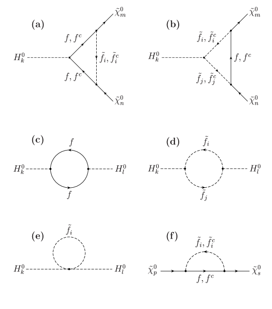
Figure 1: One-loop Feynman graphs with fermion and sfermion exchange contributing to the neutral Higgs boson-neutralino-neutralino decay amplitude. The superscript “$c$” denotes the charge conjugated states.

The abbreviations $B_{0}=B_{0}(m_{H^{0}_{k}}^{2},m_{f}^{2},m_{f}^{2})$, $C^{i}_{..}=C_{..}(m_{m}^{2},m_{H^{0}_{k}}^{2},m_{n}^{2},m_{{\tilde{f}}_{i}}^{2},m_{f}^{2},m_{f}^{2})$, and $C^{ij}_{..}=C_{..}(m_{m}^{2},m_{H^{0}_{k}}^{2},m_{n}^{2},m_{f}^{2},m_{{\tilde{f}}_{i}}^{2},m_{{\tilde{f}}_{j}}^{2})$ have been used.

The wave-function correction is given by

$$\delta{F}_{mnk}^{0\,(w)}\,=\,\frac{\,1}{\,2}\,\bigg{[}\,\delta{Z}^{H^{0}}_{lk}{F}_{mnl}^{0}+\delta{Z}_{qm}^{{\tilde{\chi}}}{F}_{qnk}^{0}+\delta{Z}_{qn}^{{\tilde{\chi}}}{F}_{mqk}^{0}\bigg{]}\,,$$ (12)

with the implicit summations over $l=1,2$ for k = 1 or 2, $l=3,4$ for $k=3$, and $q=1,\ldots,4$. $\delta{Z}^{{\tilde{\chi}}}$ are the wave-function constant terms for the neutralinos given in (20), (21). The wave-function constant terms for the Higgs bosons $\delta{Z}^{H^{0}}$ are

$$\delta{Z}^{H^{0}}_{kk} = -\;{\rm Re}\,\dot{\Pi}^{H^{0}}_{kk}(m_{H_{k}^{0}}^{2})\,,$$ (13)

$$\delta{Z}^{H^{0}}_{kl} = \frac{1}{m^{2}_{H_{k}^{0}}-m^{2}_{H_{l}^{0}}}\,{\rm Re}\,\bigg{\{}\Pi^{H^{0}}_{kl}(m^{2}_{H_{l}^{0}})-\Pi^{H^{0}}_{kl}(m^{2}_{H_{k}^{0}})\bigg{\}}\,,\hskip 56.9055ptl\neq{k}\,,$$ (14)

with $k,l=1,2$ for the system $(h^{0},H^{0})$ and $k,l=3,4$ for $(A^{0},G^{0})$. Eq. (14) has been symmetrized with respect to $(k,l)$. This is due to the on-shell renormalization of the Higgs mixing angle $\alpha$ ($k,l=1,2$) or $\beta$ ($k,l=3,4$). In this scheme ([11], extending [17] for quark and lepton mixing) the counter terms for the mixing angles are determined by the requirement that they cancel the antisymmetric parts of the wave-function corrections.

The decays of $A^{0}$ are a little complicated by the contribution of the $A^{0}-Z^{0}$ mixing in addition to the $A^{0}-G^{0}$ mixing in eq. (14). Moreover, both depend on the gauge parameter $\xi$. However, the sum of these two contributions is independent of $\xi$, as it is shown in Appendix C. Here we work in the $\xi=0$ (Landau) gauge, where the contribution of the $A^{0}-Z^{0}$ mixing vanishes, and use (14) with $m_{H^{0}_{4}}=0$. The resulting on-shell $\tan\beta$ agrees with the one defined by the $A^{0}$–$Z^{0}$ mixing [18, 19, 11].

The Higgs self-energy contributions due to fermions and sfermions are written as

$$\Pi^{H^{0}}_{kl}(k^{2})=\Pi^{H^{0}\,(a)}_{kl}(k^{2})+\Pi^{H^{0}\,(b)}_{kl}(k^{2})+\Pi^{H^{0}\,(c)}_{kl}+T_{kl}\,.$$ (15)

The fermion contribution $\Pi^{H^{0}\,(a)}$ (Fig. 1c) is

$$\Pi^{H^{0}\,(a)}_{ab}(k^{2}) = \frac{2\,s^{f}_{a}\,s^{f}_{b}}{\left(4\pi\right)^{2}}\,\bigg{[}\Big{(}k^{2}-4m_{f}^{2}\Big{)}\,B_{0}(k^{2},m_{f}^{2},m_{f}^{2})-2A_{0}(m_{f}^{2})\bigg{]}\,,$$ (16)

$$\Pi^{H^{0}\,(a)}_{cd}(k^{2}) = -\frac{2\,s^{f}_{c}\,s^{f}_{d}}{\left(4\pi\right)^{2}}\,\bigg{[}k^{2}\,B_{0}(k^{2},m_{f}^{2},m_{f}^{2})-2A_{0}(m_{f}^{2})\bigg{]}\,,$$ (17)

with $a,b=1,2$ and $c,d=3,4$. The sfermion contributions $\Pi^{H^{0}\,(b)}$ (Fig. 1d) and $\Pi^{H^{0}\,(c)}$ (Fig. 1e) are

$$\Pi^{H^{0}\,(b)}_{kl}(k^{2}) = \frac{1}{\left(4\pi\right)^{2}}\;\sum_{i,j=1}^{2}G^{{\tilde{f}}}_{jik}\,G^{{\tilde{f}}}_{ijl}\;B_{0}(k^{2},m_{{\tilde{f}}_{i}}^{2},m_{{\tilde{f}}_{j}}^{2})\,,$$ (18)

$$\Pi^{H^{0}\,(c)}_{kl} = {\frac{1}{\left(4\pi\right)^{2}}}\;\sum_{i=1}^{2}\bigg{[}h_{f}^{2}\,c_{kl}^{\tilde{f}}\,+\,g^{2}d_{kl}\,e_{ii}^{\tilde{f}}\bigg{]}A_{0}(m_{{\tilde{f}}_{i}}^{2})\,,$$ (19)

where $k,l=1,2$ or $3,4$. $T_{kl}$ in eq. (15) represent momentum-independent contributions from the tadpole shifts [18, 19] and leading higher-order corrections. We include the latter by the renormalization group improvement as in Ref. [20]. Since the zero-momentum contribution $\Pi^{H^{0}}_{kl}(0)$, including $T_{kl}$, is very large it is often resummed as in Refs. [19, 21]. In practice, we calculate the effective $m_{H^{0}_{a}}(a=1,2)$ and $\alpha$ obtained from the effective mass matrix, which includes the $\Pi^{H^{0}}_{ab}(k^{2}=0)$ contribution with $m_{A^{0}}$, $\tan\beta$, and the (s)quark parameters, and regard them as the lowest-order parameters. If one is replacing $\alpha$ in all the previous formulae with the effective one, the self energies $\Pi^{H^{0}}_{kl}(k^{2})$ in the wave-function correction and $\delta\alpha$ must be replaced by $\Delta\Pi^{H^{0}}_{kl}(k^{2})=\Pi^{H^{0}}_{kl}(k^{2})-\Pi^{H^{0}}_{kl}(0)$. Nevertheless, the form of their sums eqs. (13,14) is not affected by the elimination of $\Pi^{H^{0}}_{kl}(0)$.

The neutralino wave-function terms read

$$\delta{Z}^{{\tilde{\chi}}}_{pp} = -\;{\rm Re}\,\bigg{\{}\Pi^{{\tilde{\chi}}}_{pp}(m_{p}^{2})+2m_{p}\,\Big{[}m_{p}\dot{\Pi}^{{\tilde{\chi}}}_{pp}(m_{p}^{2})+m_{f}\dot{\Pi}^{{\tilde{\chi}}_{S}}_{pp}(m_{p}^{2})\Big{]}\bigg{\}}\,,$$ (20)

$$\delta{Z}^{{\tilde{\chi}}}_{ps} = \frac{1}{m_{p}-m_{s}}\;{\rm Re}\bigg{\{}m_{s}\left[\Pi^{{\tilde{\chi}}}_{ps}(m_{s}^{2})-\Pi^{{\tilde{\chi}}}_{ps}(m_{p}^{2})\right]+m_{f}\left[\Pi^{{\tilde{\chi}}\,S}_{ps}(m_{s}^{2})-\Pi^{{\tilde{\chi}}\,S}_{ps}(m_{p}^{2})\right]\bigg{\}}\,,$$ (21)

$p\neq s$. As before, $\delta{Z}^{{\tilde{\chi}}}_{ps}$ in (21) has been symmetrized by subtracting the counter term for the rotation matrix $Z$ of the neutralinos [11]. The neutralino self-energies due to the sfermion-fermion loop (Fig. 1f ) are

$$\Pi^{\tilde{\chi}}_{ps}(k^{2}) = -\frac{1}{(4\pi)^{2}}\,\sum_{i=1}^{2}(a^{\tilde{f}}_{ip}a^{\tilde{f}}_{is}+b^{\tilde{f}}_{ip}b^{\tilde{f}}_{is})\,B_{1}(k^{2},m_{f}^{2},m_{{\tilde{f}}_{i}}^{2})\,,$$ (22)

$$\Pi^{{\tilde{\chi}}\,S}_{ps}(k^{2}) = \frac{1}{(4\pi)^{2}}\,\sum_{i=1}^{2}(a^{\tilde{f}}_{ip}b^{\tilde{f}}_{is}+a^{\tilde{f}}_{is}b^{\tilde{f}}_{ip})\,B_{0}(k^{2},m_{f}^{2},m_{{\tilde{f}}_{i}}^{2})\,,$$ (23)

see also [20].

We need the counter term for the couplings $gF^{0}_{mnk}$, which is a function of the gauge couplings $g$, $g^{\prime}$, the Higgs boson mixing angle $\alpha$ (for $k=1,2$) or $\beta$ (for $k=3$), and the neutralino rotation matrix $Z$, as shown in eq. (A.2). The counter terms for ($\alpha$, $\beta$) and $Z$ in the on-shell scheme [11] are already included in the wave-function corrections (14) and (21), respectively. The remaining counter term of $\delta g$ and $\delta g^{\prime}$ is, after being absorbed into the correction to $F^{0}_{mnk}$,

$$\delta F^{0\,(c)}_{mnk} = \sum_{x=3,4}\,d^{x}_{k}\left[\left(Z_{mx}Z_{n2}+Z_{m2}Z_{nx}\right)\,\frac{\delta g}{g}-\left(Z_{mx}Z_{n1}+Z_{m1}Z_{nx}\right)\,\tan\theta_{W}\,\frac{\delta g^{\prime}}{g^{\prime}}\right]\,.$$ (24)

We fix the electroweak gauge boson sector by $m_{Z}$, $m_{W}$, and $e$. One gets from the relations $g=e/s_{W}$, $g^{\prime}=e/c_{W}$, and $c_{W}={m_{W}}/{m_{Z}}$ ($c_{W}\equiv\cos\theta_{W}$, $s_{W}\equiv\sin\theta_{W}$) [22, 16]

$$\frac{\delta g}{g}=\frac{\delta e}{e}+\frac{c_{W}^{2}}{2\,s_{W}^{2}}\left(\frac{\delta m_{W}^{2}}{m_{W}^{2}}-\frac{\delta m_{Z}^{2}}{m_{Z}^{2}}\right)\,,\hskip 42.67912pt\frac{\delta g^{\prime}}{g^{\prime}}=\frac{\delta e}{e}-\frac{1}{2}\left(\frac{\delta m_{W}^{2}}{m_{W}^{2}}-\frac{\delta m_{Z}^{2}}{m_{Z}^{2}}\right)\,.$$ (25)

The formulae for $\delta m_{W}$ and $\delta m_{Z}$ can be also found in [11] and for $\delta e/e$ in the Appendix B.

Now all parts are given which are needed in order to calculate the (UV finite) one-loop contribution to the neutral Higgs boson-neutralino-neutralino coupling, eq. (8). The vertex correction part $\delta F^{0\,(v)}_{mnk}$ is given by eqs. (10) and (11), the wave-function correction term $\delta F^{0\,(w)}_{mnk}$ by eq. (12), and $\delta F^{0\,(c)}_{mnk}$ by eq. (24).

Further, one has to note that the on-shell masses and the mixing of the neutralinos are not independent of each other. In fact, when the gauge and Higgs boson sectors are fixed, the neutralino sector is determined by three free parameters only. Here we follow the method given by [11]: The on-shell mass parameters $M$ and $\mu$ are defined as the elements of the on-shell mass matrix $X$ of charginos, and the on-shell mass parameter $M^{\prime}$ is defined as the element of the on-shell mass matrix $Y$ of neutralinos . The finite correction $\Delta Y=Y-Y^{\rm tree}$, where $Y^{\rm tree}$ is the tree-level mass matrix in terms of the on-shell parameters $(M,\mu,M^{\prime},m_{Z},\sin\theta_{W},\tan\beta)$, is calculated by eqs. (42–51) in [11]. The one-loop corrected on-shell masses $m_{i}$ and mixing matrix $Z=Z^{\rm tree}+\Delta Z$ are then obtained by diagonalizing $Y$. For a proper treatment of the loop corrections, the resulting shifts of the masses and the mixing matrix from the tree-level values have to be taken into account.

4 Numerical results

For simplicity, we will take in the following (if not specified otherwise) for the soft breaking sfermion mass parameters of the first, second and third generation $M_{\tilde{Q}_{1,2}}=M_{\tilde{U}_{1,2}}=M_{\tilde{D}_{1,2}}=M_{\tilde{L}_{1,2}}=M_{\tilde{E}_{1,2}}=M_{\tilde{Q}_{3}}=\frac{10}{9}M_{\tilde{U}_{3}}=\frac{10}{11}M_{\tilde{D}_{3}}=M_{\tilde{L}_{3}}=M_{\tilde{E}_{3}}=M_{\tilde{Q}}=500$ GeV and for the trilinear couplings $A_{t}=A_{b}=A_{\tau}=A=300$ GeV. We take $m_{Z}=91.2$ GeV, $m_{W}=80$ GeV, $m_{A^{0}}=500$ GeV, $m_{t}=175$ GeV, $m_{b}=5$ GeV, and $m_{\tau}=1.8$ GeV. Masses of all other SM fermions are neglected. We use the GUT relations $M^{\prime}=\frac{5}{3}\tan^{2}{\theta_{W}}\,M$ and for the gluino mass $m_{\tilde{g}}=({\alpha_{S}}/{\alpha_{EW}})\sin^{2}{\theta_{W}}\,M$. The other input parameters are $\{\,\tan{\beta},\,M,\,\mu\}$ (all as on-shell parameters). For the values of the Yukawa couplings of the $3^{\rm rd}$ quark generation ($h_{t}$, $h_{b}$), we take the running ones at the scale of the decaying particle mass.

In our numerical analysis we have discussed four cases: the tree-level width, the corrections (7–9) with the tree-level $Z$ and $m_{i}$ (“conventional correction”), the corrections (7–9) with the one-loop corrected $Z$ and tree-level $m_{i}$ (“conventional $+$ $\Delta Z$ correction”), and the corrections (7–9) with the one-loop corrected $Z$ and one-loop corrected $m_{i}$ (full correction). The “conventional correction” corresponds to the correction to the gaugino-higgsino-Higgs boson coupling, “conventional $+$ $\Delta Z$ correction” includes the correction to the neutralino components, and the correction due to the shift of $m_{i}$ is added in the full correction.

In Fig. 2a we show, as a function of $\mu$, the tree-level widths of $H^{0}\to{\tilde{\chi}}^{0}_{1}+{\tilde{\chi}}^{0}_{2}$, $H^{0}\to{\tilde{\chi}}^{0}_{1}+{\tilde{\chi}}^{0}_{3}$ and $H^{0}\to{\tilde{\chi}}^{0}_{2}+{\tilde{\chi}}^{0}_{2}$, respectively, for $\tan{\beta}=10$ and $M=150$ GeV. The $H^{0}$ mass is $m_{H^{0}}\sim 500$ GeV. The widths vary with the gaugino and higgsino components of the various neutralino states. Fig. 2b exhibits the corrections to the width of $H^{0}\to{\tilde{\chi}}^{0}_{1}+{\tilde{\chi}}^{0}_{2}$: The “conventional”, “conventional $+\Delta Z$”, and full corrections are shown. One can see that, compared to the “conventional” correction, the corrections by the shifts $\Delta Z$ and $m_{i}$ cannot be neglected. Figs. 2c and 2d show the corrections to the widths of $H^{0}\to{\tilde{\chi}}^{0}_{1}+{\tilde{\chi}}^{0}_{3}$ and $H^{0}\to{\tilde{\chi}}^{0}_{2}+{\tilde{\chi}}^{0}_{2}$, respectively. While the “conventional” correction is dominant for $\mu<0$ in Fig. 2c, the “$\Delta Z$” correction is dominant in Fig. 2d. The full corrections amount to several %.

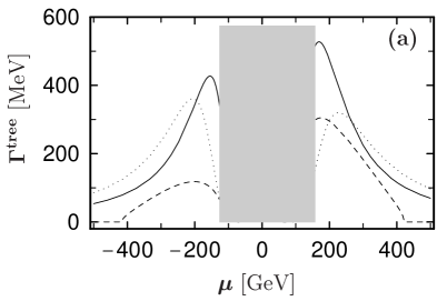
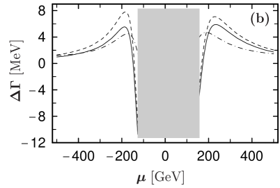
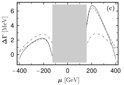
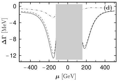
Figure 2: Tree-level widths (a) of the decays $H^{0}\to{\tilde{\chi}}^{0}_{1}+{\tilde{\chi}}^{0}_{2}$ (solid), $H^{0}\to{\tilde{\chi}}^{0}_{1}+{\tilde{\chi}}^{0}_{3}$ (dashed) and $H^{0}\to{\tilde{\chi}}^{0}_{2}+{\tilde{\chi}}^{0}_{2}$ (dotted) and corrections to the widths of these decays (b), (c), and (d), respectively, as a function of $\mu$ for $\tan{\beta}=10$ and $M=150$ GeV. The full, dashed, dash-dotted line corresponds to the full, “conventional + $\Delta{Z}$”, and “conventional” correction. The grey areas are excluded by the bounds $m_{{\tilde{\chi}}^{\pm}_{1}}\geq 100$ GeV, $m_{h^{0}}>92$ GeV.

In Fig. 3, we show the tree and corrected widths of (a) $H^{0}\to{\tilde{\chi}}^{0}_{1}+{\tilde{\chi}}^{0}_{2}$ decay with $\tan\beta=10$, $M=500$ GeV and $\mu=150$ GeV, and those of (b) $A^{0}\to{\tilde{\chi}}^{0}_{1}+{\tilde{\chi}}^{0}_{3}$ decay with $\tan\beta=50$ and $M=\mu=300$ GeV, as functions of $M_{\tilde{Q}}$. In Fig. 3a, the decay is suppressed due to the small gaugino components of ${\tilde{\chi}}^{0}_{1}$ and ${\tilde{\chi}}^{0}_{2}$. The “conventional$+\Delta Z$” correction is close to the full correction and therefore not shown here. We see that the “conventional” correction is dominant. In contrast, the “$\Delta m$” correction in Fig. 3b is large and negative (up to $-16$%), which dominates over the positive “conventional” correction (up to $+4$%). This is because the decay in Fig. 3b is kinematically suppressed and sensitive to the shift of $m_{i}$. We note that the sfermion loop corrections do not decouple in large $M_{\tilde{Q}}$ limit, due to the supersymmetry breaking corrections [23] to the gaugino-higgsino-Higgs boson couplings.

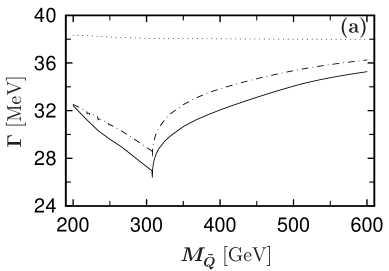
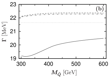
Figure 3: The widths of the decays $H^{0}\to{\tilde{\chi}}^{0}_{1}+{\tilde{\chi}}^{0}_{2}$ (a) and $A^{0}\to{\tilde{\chi}}^{0}_{1}+{\tilde{\chi}}^{0}_{3}$ (b) as a function of $M_{\tilde{Q}}$. The dotted line corresponds to the tree-level width, the dash-dotted, dashed, and solid line corresponds to the “conventional”, “conventional + $\Delta{Z}$”, and full correction, respectively. The parameters are $\tan{\beta}=10$, $M=500$ GeV, and $\mu=150$ GeV (a) and $\tan{\beta}=50$ and $M=\mu=300$ GeV (b).

Figs. 4a and 4b show the dependence of the widths on the trilinear coupling $A$ for the same decays modes and parameter sets as in Figs. 3a and 3b, respectively. The $A$ dependence is mainly caused by $A_{t}$ and numerically important in general.

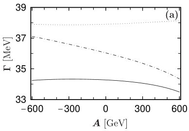
Figure 4: The widths of the decays $H^{0}\to{\tilde{\chi}}^{0}_{1}+{\tilde{\chi}}^{0}_{2}$ (a) and $A^{0}\to{\tilde{\chi}}^{0}_{1}+{\tilde{\chi}}^{0}_{3}$ (b) as a function of $A$. The dotted line corresponds to the tree-level width, the dash-dotted, dashed and solid line corresponds to the “conventional”, “conventional + $\Delta{Z}$”, and full correction, respectively. The parameters are $\tan{\beta}=10$, $M=500$ GeV, and $\mu=150$ GeV (a) and $\tan{\beta}=50$ and $M=\mu=300$ GeV (b).

We also discuss the related decays (3) of the neutralinos. In Figs. 5a and 5b we show the corrections to the width of the decays ${\tilde{\chi}}^{0}_{3}\to h^{0}+{\tilde{\chi}}^{0}_{1}$ and ${\tilde{\chi}}^{0}_{4}\to h^{0}+{\tilde{\chi}}^{0}_{1}$ as functions of $M_{\tilde{Q}}$ and $A$, respectively. The parameters are as in Fig. 3a for Fig. 5a and $\tan{\beta}=10$ and $M=\mu=300$ GeV for Fig. 5b. The total correction can go up to 25%.

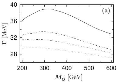
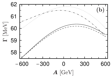
Figure 5: The widths of the decays ${\tilde{\chi}}^{0}_{3}\to h^{0}+{\tilde{\chi}}^{0}_{1}$ (a) and ${\tilde{\chi}}^{0}_{4}\to h^{0}+{\tilde{\chi}}^{0}_{1}$ (b) as a function of $M_{\tilde{Q}}$ (a) and $A$ (b). The dotted line corresponds to the tree-level width, the dash-dotted, dashed and solid line correspond to the “conventional”, “conventional + $\Delta{Z}$”, and full corrections, respectively. The parameters are $\tan{\beta}=10$, $M=500$ GeV, and $\mu=150$ GeV (a) and $\tan{\beta}=10$ and $M=\mu=300$ GeV (b).

Finally, Fig. 6 shows the $\mu$ dependence of the width of the decay $h^{0}\to{\tilde{\chi}}^{0}_{1}+{\tilde{\chi}}^{0}_{1}$ (1), both the tree-level value (Fig. 6a) and the relative one-loop full correction (Fig. 6b). This decay occurs when $\tilde{\chi}^{0}_{1}$ is sufficiently light and is mainly a U(1) gaugino to escape from the present direct search. In order to realize this case, we consider very small $M^{\prime}$ and take the following parameters which are similar to those in Ref. [7]: $M_{\tilde{Q}_{1,2}}=M_{\tilde{U}_{1,2}}=M_{\tilde{D}_{1,2}}=M_{\tilde{Q}_{3}}=M_{\tilde{U}_{3}}=M_{\tilde{D}_{3}}=2M_{\tilde{L}_{1,2}}=2M_{\tilde{E}_{1,2}}=2M_{\tilde{L}_{3}}=2M_{\tilde{E}_{3}}=500$ GeV, $A_{t}=1000$ GeV, $A_{b}=A_{\tau}=0$ GeV, $M^{\prime}=30$ GeV, $M=120$ GeV, $m_{\tilde{g}}=500$ GeV, $\tan\beta=20$, and $m_{A^{0}}=300$ GeV. The loop correction can be comparable to or even larger than the tree-level width as observed in Ref. [7]. Although the decay width is much smaller than the other modes, the effect of the loop correction might be seen in precision studies of $h^{0}$ at a linear collider [7] and in neutralino dark matter search [7, 8, 9].

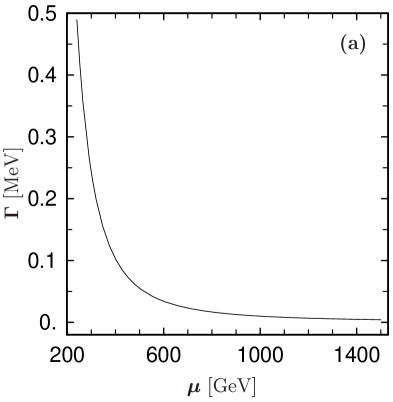
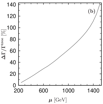
Figure 6: The tree-level width (a) and the relative full correction (b) of the decay$h^{0}\to{\tilde{\chi}}^{0}_{1}+{\tilde{\chi}}^{0}_{1}$ as a function of $\mu$ for the parameters $\tan\beta=20$, $\{M,\,M^{\prime},\,m_{\tilde{g}},\,m_{A^{0}}\}=\{120,\,30,\,500,\,300\}$ GeV, $\{A_{t},\,A_{b},\,A_{\tau}\}=\{1,\,0,\,0\}$ TeV, and $M_{\tilde{Q}_{1,2}}=M_{\tilde{U}_{1,2}}=M_{\tilde{D}_{1,2}}=M_{\tilde{Q}_{3}}=M_{\tilde{U}_{3}}=M_{\tilde{D}_{3}}=2M_{\tilde{L}_{1,2}}=2M_{\tilde{E}_{1,2}}=2M_{\tilde{L}_{3}}=2M_{\tilde{E}_{3}}=500$ GeV.

5 Conclusions

We have presented the calculation of the one-loop corrections to the decays$(h^{0},H^{0},A^{0})\to{\tilde{\chi}}^{0}_{m}+{\tilde{\chi}}^{0}_{n}$ and ${\tilde{\chi}}^{0}_{m}\to(h^{0},H^{0},A^{0})+{\tilde{\chi}}^{0}_{n}$, $(m,n=1,\ldots,4)$, with all fermions and sfermions in the loop. These decays are special in the sense that they require particular care in the treatment of the neutralino mixing and mass matrix in a scheme, where all parameters in the neutralino mass matrix $Y$ and mixing matrix $Z$ are defined on-shell. We have shown the importance of the corrections to these matrices in addition to the conventional corrections (vertex and wave-function corrections with counter terms). We have studied the dependence on the parameters $M$, $\mu$, $A$, $M_{\tilde{Q}}$, and $\tan\beta$. The corrections to the widths of the decays $(h^{0},H^{0},A^{0})\to{\tilde{\chi}}^{0}_{m}+{\tilde{\chi}}^{0}_{n}$ can go up to $\sim$ 15%, those of the decays ${\tilde{\chi}}^{0}_{m}\to(h^{0},H^{0},A^{0})+{\tilde{\chi}}^{0}_{n}$ to $\sim$ 25%. For the invisible decay $h^{0}\to{\tilde{\chi}}^{0}_{1}+{\tilde{\chi}}^{0}_{1}$, giving up the GUT relation for $M^{\prime}$, one even gets corrections up to 140%.

Appendix

In the following we give the formulae for the couplings and for $\delta e$. Furthermore, the proof of the gauge independence of the processes considered will be given.

Appendix A Coupling parameters

The $H^{0}_{k}\,{\tilde{\chi}^{0}}_{m}\,{\tilde{\chi}^{0}}_{n}$ interaction is given by

$${\cal L}=-\frac{1}{2}\,g\,H^{0}_{a}\,\bar{\tilde{\chi}}^{0}_{m}\,F^{0}_{mna}\,{\tilde{\chi}^{0}}_{n}+\frac{i}{2}\,g\,H^{0}_{c}\,\bar{\tilde{\chi}}^{0}_{m}\,F^{0}_{mnc}\,\gamma^{5}\,{\tilde{\chi}^{0}}_{n}\,,$$ (A.1)

with $a=1,2$, $c=3,4$, and

$$F^{0}_{mnk} = \hphantom{+}\frac{d^{u}_{k}}{2}\,\bigg{[}Z_{m4}Z_{n2}+Z_{n4}Z_{m2}-{\tan{\theta_{W}}}(Z_{m4}Z_{n1}+Z_{n4}Z_{m1})\bigg{]}$$ (A.2)

$$+\frac{d^{d}_{k}}{2}\,\bigg{[}Z_{m3}Z_{n2}+Z_{n3}Z_{m2}-{\tan{\theta_{W}}}(Z_{m3}Z_{n1}+Z_{n3}Z_{m1})\bigg{]}\,.$$

The $Z_{mn}$ are the elements of the neutralino mixing matrix which diagonalizes the neutralino mass matrix and

$$d_{k}^{4}=d^{u}_{k} = \Big{(}-{\cos{\alpha}},\,-{\sin{\alpha}},\,\hphantom{-}{\cos{\beta}},\,\hphantom{-}{\sin{\beta}}\Big{)}_{k}\,,$$

$$d_{k}^{3}=d^{d}_{k} = \Big{(}-{\sin{\alpha}},\,\hphantom{-}{\cos{\alpha}},\,-{\sin{\beta}},\,\hphantom{-}{\cos{\beta}}\Big{)}_{k}\,.$$ (A.3)

The superscript “$u$” denotes an up-type and “$d$” a down-type fermion.

The neutral Higgs boson-fermion-fermion couplings, defined by ${\cal L}=s^{f}_{k}\,H_{k}^{0}\,\bar{f}\,f$ are

$$s^{u}_{a}=\frac{h_{u}}{\sqrt{2}}\;d^{u}_{a}\,,\hskip 28.45274pts^{u}_{c}=i\,\frac{h_{u}}{\sqrt{2}}\;d^{u}_{c}\,,\hskip 28.45274pts^{d}_{a}=-\,\frac{h_{d}}{\sqrt{2}}\;d^{d}_{a}\,,\hskip 28.45274pts^{d}_{c}\;=\;-\,i\,\frac{h_{d}}{\sqrt{2}}\;d^{d}_{c}\,,$$ (A.4)

with $a=1,2$ and $c=3,4$, using the Yukawa couplings

$$h_{u}=\frac{g\,m_{u}}{\sqrt{2}\,m_{W}\sin\beta}\,,\hskip 28.45274pth_{d}=\frac{g\,m_{d}}{\sqrt{2}\,m_{W}\cos\beta}\,.$$ (A.5)

The fermion-sfermion-neutralino coupling parameters $a^{{\tilde{f}}}_{ip}$ and $b^{{\tilde{f}}}_{ip}$ ($i=1,2,\,p=1,\ldots,4$) have the form

$$a^{{\tilde{f}}}_{ip} = gf_{Lp}^{f}R^{\tilde{f}}_{i1}+h_{f}Z_{px}R^{\tilde{f}}_{i2}\,,$$ (A.6)

$$b^{{\tilde{f}}}_{ip} = gf_{Rp}^{f}R^{\tilde{f}}_{i2}+h_{f}Z_{px}R^{\tilde{f}}_{i1}\,,$$ (A.7)

with $x=3$ for down-type and $x=4$ for up-type fermions, $R^{\tilde{f}}$ the $2\times 2$ sfermion rotation matrix,

$$f_{Lp}^{f} = \sqrt{2}\,\bigg{[}\Big{(}e_{f}-{I_{f}^{3L}}\Big{)}{\tan{\theta_{W}}}Z_{p1}+{I_{f}^{3L}}Z_{p2}\bigg{]}\,,$$ (A.8)

$$f_{Rp}^{f} = -\sqrt{2}\,e_{f}\,{\tan{\theta_{W}}}\,Z_{p1}\,.$$ (A.9)

${I_{f}^{3L}}$ denotes the SU(2)_L isospin and $e_{f}$ the charge of the fermion $f$.

The $H^{0}_{k}\,{\tilde{f}}_{i}^{*}\,{\tilde{f}}_{j}$ couplings [2] are

$$G_{ij1}^{\tilde{u}}\equiv G(h^{0}\,{\tilde{u}}_{i}^{*}\,{\tilde{u}}_{j})=\left(R^{\tilde{u}}\,G^{\tilde{u}}_{LR1}\,(R^{{\tilde{u}}})^{T}\right)_{ij}=$$

$$-gR^{{\tilde{u}}}\left(\begin{array}[]{cc}-\frac{m_{Z}}{c_{W}}(I_{u}^{3L}-e_{u}s_{W}^{2}){\mbox{s}}_{\alpha+\beta}+\frac{m_{u}^{2}}{m_{W}{\mbox{s}}_{\beta}}{\mbox{c}}_{\alpha}&\frac{m_{u}}{2m_{W}{\mbox{s}}_{\beta}}(A_{u}{\mbox{c}}_{\alpha}+\mu{\mbox{s}}_{\alpha})\\ \frac{m_{u}}{2m_{W}{\mbox{s}}_{\beta}}(A_{u}{\mbox{c}}_{\alpha}+\mu{\mbox{s}}_{\alpha})&-\frac{m_{Z}}{c_{W}}e_{u}s_{W}^{2}{\mbox{s}}_{\alpha+\beta}+\frac{m_{u}^{2}}{m_{W}{\mbox{s}}_{\beta}}{\mbox{c}}_{\alpha}\end{array}\right)(R^{{\tilde{u}}})^{T}\,,$$ (A.12)

$$G_{ij1}^{\tilde{d}}\equiv G(h^{0}\,{\tilde{d}}_{i}^{*}\,{\tilde{d}}_{j})=\left(R^{\tilde{d}}\,G^{\tilde{d}}_{LR1}\,(R^{{\tilde{d}}})^{T}\right)_{ij}=$$

$$gR^{{\tilde{d}}}\left(\begin{array}[]{cc}\frac{m_{Z}}{c_{W}}(I_{d}^{3L}-e_{d}s_{W}^{2}){\mbox{s}}_{\alpha+\beta}+\frac{m_{d}^{2}}{m_{W}{\mbox{c}}_{\beta}}{\mbox{s}}_{\alpha}&\frac{m_{d}}{2m_{W}{\mbox{c}}_{\beta}}(A_{d}{\mbox{s}}_{\alpha}+\mu{\mbox{c}}_{\alpha})\\ \frac{m_{d}}{2m_{W}{\mbox{c}}_{\beta}}(A_{d}{\mbox{s}}_{\alpha}+\mu{\mbox{c}}_{\alpha})&\frac{m_{Z}}{c_{W}}e_{d}s_{W}^{2}{\mbox{s}}_{\alpha+\beta}+\frac{m_{d}^{2}}{m_{W}{\mbox{c}}_{\beta}}{\mbox{s}}_{\alpha}\end{array}\right)(R^{{\tilde{d}}})^{T}\,,$$ (A.15)

$$G_{ij2}^{\tilde{f}}\equiv G(H^{0}\,{\tilde{f}}_{i}^{*}\,{\tilde{f}}_{j})=G(h^{0}{\tilde{f}}_{i}^{*}{\tilde{f}}_{j})\mbox{ with }\alpha\to\alpha-\frac{\pi}{2}\,,$$ (A.16)

(i. e. $\ \sin\alpha\equiv{\mbox{s}}_{\alpha}\to-{\mbox{c}}_{\alpha}\,,\ \cos\alpha\equiv{\mbox{c}}_{\alpha}\to{\mbox{s}}_{\alpha}\,,\ \mbox{and}\;\sin(\alpha+\beta)\equiv{\mbox{s}}_{\alpha+\beta}\to-{\mbox{c}}_{\alpha+\beta})$,

$$G_{ij3}^{\tilde{u}} = G(A^{0}\,{\tilde{u}}_{i}^{*}\,{\tilde{u}}_{j})=\frac{ig}{2m_{W}}\left(\begin{array}[]{cc}\hphantom{-}0&1\\ -1&0\end{array}\right)_{ij}\,m_{u}(A_{u}\cot\beta+\mu)\,,$$ (A.19)

$$G_{ij3}^{\tilde{d}} = G(A^{0}{\tilde{d}}_{i}^{*}{\tilde{d}}_{j})=\frac{ig}{2m_{W}}\left(\begin{array}[]{cc}\hphantom{-}0&1\\ -1&0\end{array}\right)_{ij}\,m_{d}(A_{d}\tan\beta+\mu)\,,$$ (A.22)

$$G_{ij4}^{\tilde{f}}\equiv G(G^{0}\,{\tilde{f}}_{i}^{*}\,{\tilde{f}}_{j})=G(A^{0}{\tilde{f}}_{i}^{*}{\tilde{f}}_{j})\mbox{ with }\beta\to\beta-\frac{\pi}{2}\,,$$ (A.23)

(i. e. $\ \tan\beta\leftrightarrow-\cot\beta$). The superscript “${\tilde{u}}$” (“${\tilde{d}}$”) denotes an up-type (down-type) sfermion.

The $H^{0}_{k}\,H^{0}_{l}\,{\tilde{f}}_{i}^{*}\,{\tilde{f}}_{j}$ interaction is given by

$${\cal L}=-\frac{1}{2}\,\left(h_{f}^{2}\,c_{kl}^{\tilde{f}}\,\delta_{ij}+g^{2}\,d_{kl}\,e_{ij}^{\tilde{f}}\right)\,H^{0}_{k}\,H^{0}_{l}\,{\tilde{f}}_{i}^{*}\,{\tilde{f}}_{j}\,,$$ (A.24)

with

$$c^{\tilde{u}}_{kl} = \left(\begin{array}[]{cccc}{\cos^{2}{\alpha}}&\hphantom{-}{\cos{\alpha}}\,{\sin{\alpha}}&0&0\\ \hphantom{-}{\cos{\alpha}}\,{\sin{\alpha}}&{\sin^{2}{\alpha}}&0&0\\ 0&0&{\cos^{2}{\beta}}&\hphantom{-}{\cos{\beta}}\,{\sin{\beta}}\\ 0&0&\hphantom{-}{\cos{\beta}}\,{\sin{\beta}}&{\sin^{2}{\beta}}\\ \end{array}\right)_{kl}\,,$$ (A.29)

$$c^{\tilde{d}}_{kl} = \left(\begin{array}[]{cccc}{\sin^{2}{\alpha}}&-{\cos{\alpha}}\,{\sin{\alpha}}&0&0\\ -{\cos{\alpha}}\,{\sin{\alpha}}&{\cos^{2}{\alpha}}&0&0\\ 0&0&{\sin^{2}{\beta}}&-{\cos{\beta}}\,{\sin{\beta}}\\ 0&0&-{\cos{\beta}}\,{\sin{\beta}}&{\cos^{2}{\beta}}\\ \end{array}\right)_{kl}\,,$$ (A.34)

$$d_{kl} = c^{\tilde{d}}_{kl}-c^{\tilde{u}}_{kl}\,,$$ (A.35)

$$e_{ij}^{\tilde{f}} = \frac{1}{2\,c_{W}^{2}}\,\left[(I^{3L}_{f}-e_{f}s_{W}^{2})\,R_{i1}^{\tilde{f}}\,R_{j1}^{\tilde{f}}+e_{f}\,s_{W}^{2}\,R_{i2}^{\tilde{f}}\,R_{j2}^{\tilde{f}}\right]\,.$$ (A.36)

Appendix B Counter term $\delta e$

When we give the renormalized electric charge in the Thomson limit with the measured fine structure constant $\alpha=e_{0}^{2}/(4\pi)=1/137$, the counter term $\delta e_{0}$ is given by the general form [16]

$$\frac{\delta e_{0}}{e_{0}}=\frac{1}{2}\;\dot{\Pi}^{AA}_{T}(0)-\frac{s_{W}}{c_{W}}\,\frac{\Pi^{AZ}_{T}(0)}{m_{Z}^{2}}\,,$$ (B.1)

with the momentum derivative of the transverse photon self-energy $\dot{\Pi}^{AA}_{T}$ and the $\gamma-Z^{0}$ mixing self-energy, both for the on-shell photon ($p^{2}=0$). Fermions and sfermions do not contribute to $\Pi^{AZ}_{T}(0)$ as a consequence of the fact that the physical photon is massless to all orders. However, the contribution of light hadrons to $\dot{\Pi}^{AA}_{T}(0)$ has a large theoretical uncertainty [24, 16]. To avoid this problem, in this work we use the $\overline{\rm MS}$ running coupling at $Q=m_{Z}$, $\alpha(m_{Z})=e^{2}(m_{Z})/(4\pi)=1/129$ as input. The counter term $\delta e(m_{Z})$ then becomes

$$\frac{\delta e}{e}=\frac{e^{2}\,e_{f}^{2}}{(4\pi)^{2}}\,\left[\frac{2}{3}\left(\Delta+\log\frac{Q^{2}}{x_{f}^{2}}\right)+\sum_{i=1}^{2}\frac{1}{6}\left(\Delta+\log\frac{Q^{2}}{m_{{\tilde{f}}_{i}}^{2}}\right)\right]\,,$$ (B.2)

with $x_{f}=m_{Z}$ for all $m_{f}<m_{Z}$ and $x_{t}=m_{t}$. Here $\Delta$ denotes the UV divergence factor.

Appendix C Proof of the $\xi$ independence

We investigate the wave-function corrections to the process

$$A^{0}(p)\to{\tilde{\chi}}^{0}_{m}(k_{1})+{\tilde{\chi}}^{0}_{n}(k_{2})\,.$$ (C.1)

Both the contributions of the transitions $A^{0}\to G^{0}\to{\tilde{\chi}}^{0}_{m}+{\tilde{\chi}}^{0}_{n}$ and $A^{0}\to Z^{0}\to{\tilde{\chi}}^{0}_{m}+{\tilde{\chi}}^{0}_{n}$ have a dependence on the gauge parameter $\xi=\xi_{Z}$ in the propagators of $(G^{0},Z^{0})$. We show that the sum of these contributions is independent of $\xi$.
We start from the matrix elements in a general $R_{\xi}$ gauge,

$${\cal M}^{G} = (i\,\Pi_{AG})\frac{i}{p^{2}-\xi m_{Z}^{2}}(-gF_{mn4}^{0})\bar{u}(k_{1})\gamma^{5}v(k_{2})\,,$$ (C.2)

$${\cal M}^{Z} = (-ip^{\mu}\Pi_{AZ})\frac{i}{p^{2}-m_{Z}^{2}}\left(-g_{\mu\nu}+(1-\xi)\frac{p_{\mu}p_{\nu}}{p^{2}-\xi m_{Z}^{2}}\right)(-i\frac{g}{c_{W}}O^{{}^{\prime\prime}L}_{mn})\bar{u}(k_{1})\gamma^{\nu}\gamma^{5}v(k_{2})\,.$$

The self-energies $\Pi_{AG}$ and $\Pi_{AZ}$ by (s)fermion one-loop contributions are $\xi$ independent. The $Z^{0}{\tilde{\chi}}^{0}_{m}{\tilde{\chi}}^{0}_{n}$ couplings $O^{{}^{\prime\prime}L}_{mn}$ are

$$O^{{}^{\prime\prime}L}_{mn}=\frac{1}{2}(-Z_{m3}Z_{n3}+Z_{m4}Z_{n4})\,.$$ (C.4)

As limiting cases, ${\cal M}^{G}=0$ in the physical unitary gauge $\xi\to\infty$ and ${\cal M}^{Z}=0$ in the $\xi=0$ (Landau) gauge. Note that the tadpole contributions have to be included [18, 19] in $\Pi_{AG}$.

We can write ${\cal M}^{G}$ directly as

$${\cal M}^{G}=\frac{1}{p^{2}-\xi m_{Z}^{2}}\,g\,\Pi_{AG}(p^{2})\,F_{mn4}^{0}\,\bar{u}(k_{1})\gamma^{5}v(k_{2})\,.$$ (C.5)

For ${\cal M}^{Z}$ we first contract the Lorentz indices,

$$p^{\mu}\,\left(-g_{\mu\nu}+(1-\xi)\frac{p_{\mu}p_{\nu}}{p^{2}-\xi m_{Z}^{2}}\right)\bar{u}(k_{1})\gamma^{\nu}\gamma^{5}v(k_{2})=\left(\frac{(1-\xi)\,p^{2}}{p^{2}-\xi m_{Z}^{2}}-1\right)\,\bar{u}(k_{1}){p/}\gamma^{5}v(k_{2})\,,$$

and use $\bar{u}(k_{1}){p/}\gamma^{5}v(k_{2})=\bar{u}(k_{1})({k/}_{1}+{k/}_{2})\gamma^{5}v(k_{2})=(m_{m}+m_{n})\bar{u}(k_{1})\gamma^{5}v(k_{2})$. So we get

$${\cal M}^{Z}=-\frac{i}{p^{2}-m_{Z}^{2}}\left(\frac{(1-\xi)\,p^{2}}{p^{2}-\xi m_{Z}^{2}}-1\right)\frac{g}{c_{W}}\,\Pi_{AZ}(p^{2})\,O^{{}^{\prime\prime}L}_{mn}\,(m_{m}+m_{n})\,\bar{u}(k_{1})\gamma^{5}v(k_{2})\,.$$ (C.6)

We use the Slavnov-Taylor identity (see also [19], eq. (3.7))

$$p^{2}\,\Pi_{AZ}(p^{2})+i\,m_{Z}\,\Pi_{AG}(p^{2})=0\,,$$ (C.7)

and split the sum ${\cal M}^{G}+{\cal M}^{Z}$ in an obviously $\xi$ independent and possibly dependent part,

$${\cal M}^{G+Z} = \bigg{\{}\frac{i}{p^{2}-m_{Z}^{2}}\frac{g}{c_{W}}\,\Pi_{AZ}(p^{2})\,O^{{}^{\prime\prime}L}_{mn}\,(m_{m}+m_{n})$$ (C.8)

$$+\,i\,g\,\Pi_{AZ}(p^{2})\frac{p^{2}}{p^{2}-\xi m_{Z}^{2}}\left(\frac{F_{mn4}^{0}}{m_{Z}}-\frac{(1-\xi)}{p^{2}-m_{Z}^{2}}\frac{O^{{}^{\prime\prime}L}_{mn}}{c_{W}}(m_{m}+m_{n})\right)\bigg{\}}\,\bar{u}(k_{1})\gamma^{5}v(k_{2})\,.$$

With the relation (proved later)

$$m_{Z}\,c_{W}\,F^{0}_{mn4}=-O^{{}^{\prime\prime}L}_{mn}\,(m_{m}+m_{n})\,,$$ (C.9)

we get for the part written in the brackets in eq. (C.8)

$$-(m_{m}+m_{n})\frac{O^{{}^{\prime\prime}L}_{mn}}{c_{W}}\left(\frac{1}{m_{Z}^{2}}+\frac{1-\xi}{p^{2}-m_{Z}^{2}}\right)=-(m_{m}+m_{n})\frac{O^{{}^{\prime\prime}L}_{mn}}{m_{Z}^{2}\,c_{W}}\frac{p^{2}-\xi m_{Z}^{2}}{p^{2}-m_{Z}^{2}}\,,$$ (C.10)

and therefore the final result

$${\cal M}^{G+Z}=-i\,\frac{g}{m_{Z}^{2}\,c_{W}}\,\Pi_{AZ}(p^{2})\,O^{{}^{\prime\prime}L}_{mn}\,(m_{m}+m_{n})\,\bar{u}(k_{1})\gamma^{5}v(k_{2})\,.$$ (C.11)

The $\xi$ dependence is completely cancelled in (C.11).

Finally, we prove (C.9). With the abbreviation $A_{ij}=(Z_{mi}Z_{nj}+Z_{mj}Z_{ni})$ and knowing the entries of the neutralino tree-level mass matrix $Y$ (see e. g. eq. (35) in [11]), one can write $F^{0}_{mn4}$ as

$$2\,m_{Z}\,c_{W}\,F^{0}_{mn4}=Y_{13}A_{31}+Y_{23}A_{32}-Y_{14}A_{41}-Y_{24}A_{42}\,.$$ (C.12)

Next we add and subtract the terms $Y_{33}A_{33}+Y_{43}A_{34}$ and $Y_{34}A_{43}+Y_{44}A_{44}$. Exploiting the fact that $Y_{33}=Y_{44}=0$ and $Y_{34}=Y_{43}$, we get

$$2\,m_{Z}\,c_{W}\,F^{0}_{mn4}=\sum_{k}\left(Y_{k3}A_{3k}-Y_{k4}A_{4k}\right)\,.$$ (C.13)

Writing the entries of $Y$ in terms of neutralino masses, $Y_{kj}=\sum_{l}m_{l}Z_{lk}Z_{lj}$, and using $\sum_{k}Z_{ik}Z_{jk}=\delta_{ij}$ we get

$$2\,m_{Z}\,c_{W}\,F^{0}_{mn4} = \sum_{k,l}m_{l}Z_{lk}\left[Z_{l3}\left(Z_{m3}Z_{nk}+Z_{mk}Z_{n3}\right)-Z_{l4}\left(Z_{m4}Z_{nk}+Z_{mk}Z_{n4}\right)\right]$$ (C.14)

$$= \sum_{l}m_{l}\left(\delta_{nl}Z_{l3}Z_{m3}+\delta_{ml}Z_{l3}Z_{n3}-\delta_{nl}Z_{l4}Z_{m4}-\delta_{ml}Z_{l4}Z_{n4}\right)$$

$$= m_{n}Z_{n3}Z_{m3}+m_{m}Z_{m3}Z_{n3}-m_{n}Z_{n4}Z_{m4}-m_{m}Z_{m4}Z_{n4}$$

$$= \left(Z_{m3}Z_{n3}-Z_{m4}Z_{n4}\right)(m_{m}+m_{n})=-2\,O^{{}^{\prime\prime}L}_{mn}\,(m_{m}+m_{n})\,.$$

Therefore, eq. (C.9) is proven.

However, from the Slavnov-Taylor identity one can prove in general that the same cancellation of the gauge dependent parts in $G^{0}$ and $Z^{0}$ propagators occurs for any one-loop two-body decay of $A^{0}$.

References

[1]
H. P. Nilles, Phys. Rep. 110, 1 (1984);
H. E. Haber and G. L. Kane, Phys. Rep. 117, 75 (1985);
R. Barbieri, Riv. Nuov. Cim. 11, 1 (1988).
[2]
J. F. Gunion, H. E. Haber, G. L. Kane, and S. Dawson, The Higgs Hunter’s Guide,
Addison-Wesley (1990);
J. F. Gunion and H. E. Haber, Nucl. Phys. B272, 1 (1986); B402, 567(E) (1993).
[3]
H. Baer, D. Dicus, M. Drees, and X. Tata, Phys. Rev. D 36, 1363 (1987);
J. F. Gunion and H. E. Haber, Nucl. Phys. B307, 445 (1988); B402, 569(E) (1993);
K. Griest and H. E. Haber, Phys. Rev. D 37, 719 (1988).
[4]
A. Djouadi, J. Kalinowski, and P. M. Zerwas,
Z. Phys. C 57, 569 (1993);
A. Djouadi, P. Janot, J. Kalinowski, and P. M. Zerwas,
Phys. Lett. B 376, 220 (1996); A. Djouadi, J. Kalinowski, P. Ohmann, and P. M. Zerwas,
Z. Phys. C 74, 93 (1997); A. Djouadi, Mod. Phys. Lett. A 14, 359 (1999);
G. Bélanger, F. Boudjema, F. Donato, R. Godbole, and S. Rosier-Lees,
Nucl. Phys. B581, 3 (2000).
[5]
Wang Lang–Hui, Ma We–Gan, Zhang Ren–You, and Jiang Yi,
Phys. Rev. D 64, 115004 (2001).
[6]
M. Drees, M. M. Nojiri, D. P. Roy, and Y. Yamada,
Phys. Rev. D 56, 276 (1997); 64, 039901(E) (2001).
[7]
A. Djouadi, M. Drees, P. Fileviez Perez, and M. Mühlleitner,
hep-ph/0109283
[8]
M. Drees and M. M. Nojiri, Phys. Rev. D 47, 4226 (1993);
48, 3483 (1993).
[9]
G. Jungman, M. Kamionkowski, and K. Griest, Phys. Rep. 267, 195 (1996);
A. B. Lahanas, D. V. Nanopoulos, and V. C. Spanos, Mod. Phys. Lett. A
16, 1229 (2001); Phys. Lett. B 518, 94 (2001);
M. Drees, Y. G. Kim, T. Kobayashi, and M. M. Nojiri, Phys. Rev. D
63, 115009 (2001).
[10]
A. Bartl, H. Fraas, and W. Majerotto, Nucl. Phys. B278, 1 (1986);
S. Ambrosanio and B. Mele, Phys. Rev. D 52, 3900 (1995).
[11]
H. Eberl, M. Kincel, W. Majerotto, and Y. Yamada, Phys. Rev. D 64, 115013
(2001).
[12]
J. F. Gunion and H. E. Haber, Phys. Rev. D 37, 2515 (1988).
[13]
S. Ambrosanio and B. Mele, Phys. Rev. D 53, 2541 (1996).
[14] A. Bartl, W. Majerottok, and W. Porod, Phys. Lett. B 465, 187
(1999);
A. Djouadi, Y. Mambrini, and M. Mühlleitner, Eur. Phys. J. C 20, 563
(2001).
[15]
G. ’t Hooft and M. Veltman, Nucl. Phys. B153, 365 (1979);
G. Passarino and M. Veltman, Nucl. Phys. B160, 151 (1979).
[16]
A. Denner, Fortschr. Phys. 41, 307 (1993).
[17]
A. Denner and T. Sack, Nucl. Phys. B347, 203 (1990);
B. A. Kniehl and A. Pilaftsis, Nucl. Phys. B474, 286 (1996).
[18]
P. H. Chankowski, S. Pokorski, and J. Rosiek, Phys. Lett. B 274, 191 (1992);
Nucl. Phys. B423, 437; 497 (1994).
[19]
A. Dabelstein, Z. Phys. C 67, 495 (1995);
Nucl. Phys. B456, 25 (1995).
[20]
D. Pierce and A. Papadopoulos, Phys. Rev. D 50, 565 (1994);
Nucl. Phys. B430, 278 (1994).
[21]
M. Carena, M. Quirós, and C. E. M. Wagner,
Nucl. Phys. B461, 407 (1996).
[22]
A. Sirlin, Phys. Rev. D 22, 971 (1980);
K.-I. Aoki, Z. Hioki, R. Kawabe, M. Konuma, and T. Muta,
Prog. Theor. Phys. Suppl. 73, 1 (1982);
M. Böhm, H. Spiesberger, and W. Hollik,
Fortschr. Phys. 34, 687 (1986).
[23]
P. H. Chankowski, Phys. Rev. D 41, 2877 (1990);
H.-C. Cheng, J. L. Feng, and N. Polonsky, Phys. Rev. D 57, 152 (1998);
S. Kiyoura, M. M. Nojiri, D. M. Pierce, and Y. Yamada,
Phys. Rev. D 58, 075002 (1998).
[24]
H. Burkhardt, F. Jegerlehner, G. Penzo, and C. Verzegnassi,
Z. Phys. C 43, 497 (1989).