Quintessence Unification Models from Non-Abelian Gauge Dynamics

A. de la Macorra

ABSTRACT

We show that the condensates of a non-abelian gauge group, unified with the standard model gauge groups, can parameterize the present day cosmological constant and play the role of quintessence. The models agree with SN1a and recent CMB analysis.

These models have no free parameters. Even the initial energy density at the unification scale and at the condensation scale are fixed by the number of degrees of freedom of the gauge group (i.e. by $N_{c},N_{f}$). The values of $N_{c},N_{f}$ are determined by imposing gauge coupling unification and the number of models is quite limited. Using Affleck-Dine-Seiberg superpotential one obtains a scalar potential $V=\Lambda_{c}^{4+n}\phi^{-n}$. Models with $2<n<4.27$ or equivalently $2\times 10^{-2}GeV<\Lambda_{c}<6\times 10^{3}GeV$ do not satisfy the unification constrain. In fact, there are only three models and they have an inverse power potential with $6/11\leq n\leq 2/3$. Imposing primordial nucleosynthesis bounds the preferred model has $N_{c}=3,N_{f}=6$, with $n=2/3$, a condensation scale $\Lambda_{c}=4.2\times 10^{-8}GeV$ and $w_{\phi o}=-0.90$ with an average value $w_{eff}=-0.93$. Notice that the tracker solution is not a good approximation since it has $w_{tr}=-\frac{2}{n+2}=-0.75$ for $n=2/3$.

We study the evolution of all fields from the unification scale and we calculate the relevant cosmological quantities. We also discuss the supersymmetry breaking mechanism which is relevant for these models.

 

1 INTRODUCTION

The Maxima and Boomerang [3] observations on the cosmic microwave background radiation (”CMBR”) and the superonovae project SN1a [4] have lead to conclude that the universe is flat and it is expanding with an accelerating velocity. These conclusions show that the universe is now dominated by a energy density with negative pressure with $\Omega_{\phi}=0.7\pm 0.1$ and $w_{\phi}<-2/3$ [6]. New analysis on the CMBR peaks constrain the models to have $w_{\phi o}=-0.82^{+.14}_{-.11}$ [7]. This energy is generically called the cosmological constant. Structure formation also favors a non-vanishing cosmological constant consistent with SN1a and CMBR observations [5]. An interesting parameterization of this energy density is in terms of a scalar field with gravitationally interaction only called quintessence [10]. The evolution of scalar field has been widely studied and some general approach con be found in [16, 17]. The evolution of the scalar field $\phi$ depends on the functional form of its potential $V(\phi)$ and a late time accelerating universe constrains the form of the potential [17].

It is well known that the gauge coupling constant of a non-abelian asymptotically free gauge group increases with decreasing energy and the free elementary fields will eventually condense due to the strong interaction, e.g. mesons and baryons in QCD. The scale where the coupling constant becomes strong is called the condensation scale $\Lambda_{c}$ and below it there are no more free elementary fields. These condensates, e.g. ”mesons”, develop a non trivial potential which can be calculated using Affleck’s potential [23]. The potential is of the form $V=\Lambda_{c}^{4+n}\phi^{-n}$, where $\phi$ represents the ”mesons”, and depending on the value of $n$ the potential V may lead to an acceptable phenomenology. The final value of $w_{\phi o}$ (from now on the subscript ”o” refers to present day quantities) depends $n$ and the initial condition $\Omega_{\phi i}$ [27]. A $w_{\phi o}<-2/3$, which is the upper limit of [7], requires $n<2.74$ for $\Omega_{\phi i}\geq 0.25$ [27]. For smaller $\Omega_{\phi i}$ one obtains a larger $w_{\phi o}$ for a fixe $n$. The position of the third CMBR peak favors models with $n<1$ [8] and for some class of models with $V=M^{4+n}\phi^{-n}e^{\phi^{\beta}/2}$, with $n\geq 1,\beta\geq 0$, the constraint an the equation of state is even stricter $-1\leq w_{\phi o}\leq-0.93$ [9]. In this kind of inverse power potential models (i.e. $n<2$) the tracker solution is not a good approximation to the numerical solution because the scalar field has not reached its tracker value by present day.

Here we focus on a non-abelian asymptotically free gauge group whose gauge coupling constant is unified with the couplings of the standard model (”SM”) ones [15, 27]. We will call this group the quintessence or $Q$ group. The cosmological picture in this case is very pleasing. We assume gauge coupling unification at the unification scale $\Lambda_{gut}$ for all gauge groups (as predicted by string theory) and then let all fields evolve. At the beginning all fields, SM and $Q$ model, are massless and red shift as radiation until we reach the condensation scale $\Lambda_{c}$ of Q. Below this scale the fields of the quintessence gauge group will dynamically condense and we use Affleck’s potential to study its cosmological evolution. The energy density of the $Q$ group $\Omega_{\phi}$ drops quickly, independently of its initial conditions, and it is close to zero for a long period of time, which includes nucleosynthesis (NS) if $\Lambda_{c}$ is larger than the NS energy $\Lambda_{NS}$ (or temperature $T_{NS}=0.1-10MeV$), and becomes relevant only until very recently. On the other hand, if $\Lambda_{c}<\Lambda_{NS}$ than the NS bounds on relativistic degrees of freedom must be imposed on the models. Finally, the energy density of $Q$ grows and it dominates at present time the total energy density with the $\Omega_{\phi o}\simeq 0.7$ and a negative pressure $w_{\phi o}<-2/3$ leading to an accelerating universe [6].

The initial conditions at the unification scale and at the condensation scale are fixed by the number of degrees of freedom of the models given in terms of $N_{c},N_{f}$. Imposing gauge coupling unification fixes $N_{c},N_{f}$ and we do not have any free parameters in the models (but for the susy breaking mechanism which we will comment in section 3). It is surprising that such a simple model works fine.

The restriction on $N_{c},N_{f}$ by gauge unification rules out models with a condensation energy scale between $2\times 10^{-2}GeV<\Lambda_{c}<6\times 10^{3}GeV$ or for models with $2<n<4.27$ (the scale $\Lambda_{c}$ is given in terms of $H_{o}$ and $n$ by $\Lambda_{c}\simeq H_{o}^{2/(4+n)}$ [13],[27]). Since $w_{\phi o}<-2/3$ requires $n<2.74$ all models must then have $\Lambda_{c}<2\times 10^{-2}GeV$. The number of models that satisfy gauge coupling unification with a $w_{\phi o}<-2/3$ is quite limited and in fact there are only three different models [27]. All acceptable models have $n\leq 2/3$ which implies that the condensation scale is smaller than the NS scale. The preferred model has $N_{c}=3,N_{f}=6$, $n=2/3$ and it gives $w_{\phi o}=-0.90$ with an average value $w_{eff}=-0.93$ agreeing with recent CMBR analysis [7, 8].

It is worth mentioning that we have taken $\Lambda_{c}$ as the one loop renormalization energy scale (as used by Affleck et al [23]) and if we had used the all loop renormalization energy scale [24] the values of $N_{c},N_{f}$ of the models may differ slightly but the general picture remains the same, i.e. there are only a few models that satisfy the requirement of gauge coupling unification, non of them have $n>2$ and there are no free parameters.

2 Condensation Scale and Scalar Potential

We start be assuming that the universe has a matter content of the supersymmetric gauge groups $SU(1)\times SU(2)\times SU(3)\times SU(Q)$ where the first three are the SM gauge groups while the last one corresponds to the ”quintessence group” $Q$ and that the couplings are unified at $\Lambda_{gut}$ with $g_{1}=g_{2}=g_{3}=g_{Q}=g_{gut}$.

The condensation scale $\Lambda_{c}$ of a gauge group $SU(N_{c})$ with $N_{f}$ (chiral + antichiral) matter fields has in $N=1$ susy a one-loop renormalization group equation given by

$$\Lambda_{c}=\Lambda_{gut}e^{-\frac{8\pi^{2}}{b_{o}g^{2}_{gut}}}$$ (1)

where $b_{o}=3N_{c}-N_{f}$ is the one-loop beta function and $\Lambda_{gut},g_{gut}$ are the unification energy scale and coupling constant, respectively. From gauge coupling unification we know that $\Lambda_{gut}\simeq 10^{16}\mathrm{GeV}$ and $g_{gut}\simeq\sqrt{4\pi/25.7}$ [28].

A phase transition takes place at the condensation scale $\Lambda_{c}$, since the elementary fields are free fields above $\Lambda_{c}$ and condense at $\Lambda_{c}$. In order to study the cosmological evolution of these condensates, which we will call $\phi$, we use Affleck’s potential [23]. This potential is non-perturbative and exact [30].

The superpotential for a non-abelian $SU(N_{c})$ gauge group with $N_{f}$ (chiral + antichiral) massless matter fields is [23]

$$W=(N_{c}-N_{f})(\frac{\Lambda_{c}^{b_{o}}}{det<Q\tilde{Q}>})^{1/(N_{c}-N_{f})}$$ (2)

where $b_{o}$ is the one-loop beta function coefficient. Taking $det<Q\tilde{Q}>=\Pi_{j=1}^{N_{f}}\phi^{2}_{j}$ one has $W=(N_{c}-N_{f})(\Lambda_{c}^{b_{o}}\phi^{-2N_{f}})^{1/(N_{c}-N_{f})}$. The scalar potential in global supersymmetry is $V=|W_{\phi}|^{2}$, with $W_{\phi}=\partial W/\partial\phi$, giving [13, 14]

$$V=c^{2}\Lambda_{c}^{4+n}\phi^{-n}$$ (3)

with $c=2N_{f}$, $n=2+4\frac{N_{f}}{N_{c}-N_{f}}$ and $\Lambda_{c}$ is the condensation scale of the gauge group $SU(N_{c})$. The natural initial value for the condensate is $\phi_{i}=\Lambda_{c}$ since it is precisely $\Lambda_{c}$ the relevant scale of the physical process of the field binding.

In eq.(3) we have taken $\phi$ canonically normalized, however the full Kahler potential $K$ is not known and for $\phi\simeq 1$ other terms may become relevant [13] and could spoil the runaway and quintessence behavior of $\phi$. Expanding the Kahler potential as a series power $K=|\phi|^{2}+\Sigma_{i}a_{i}|\phi|^{2i}/2i$ the canonically normalized field $\phi^{\prime}$ can be approximated by $\phi^{\prime}=(K_{\phi}^{\phi})^{1/2}\phi$ and eq.(3) would be given by $V=(K_{\phi}^{\phi})^{-1}|W_{\phi}|^{2}=(2N_{f})^{2}\Lambda_{c}^{4+n}\phi^{-n}(K_{\phi}^{\phi})^{(n/2-1)}$. For $n<2$ the exponent term of $K_{\phi}^{\phi}$ is negative so it would not spoil the runaway behavior of $\phi$ [15, 27].

If we wish to study models with $0<n<2$, which are cosmologically favored [27] we need to consider the possibility that not all $N_{f}$ condensates $\phi_{i}$ become dynamical but only a fraction $\nu$ are (with $N_{f}\geq\nu\geq 1$) and we also need $N_{f}>N_{c}$ [15, 27]. It is important to point out that even though it has been argued that for $N_{f}>N_{c}$ there is no non-perturbative superpotential $W$ generated [23], because the determinant of $Q\tilde{Q}$ in eq.(2) vanishes, this is not necessarily the case [25]. If we consider the elementary quarks $Q_{i}^{\alpha},\tilde{Q}_{i}^{\alpha}$ ($i,j=1,2,...,N_{f},\;\alpha=1,2,...,N_{c}$) to be the relevant degrees of freedom, then for $N_{c}<N_{f}$ the quantity $det(Q^{i}_{\alpha}\tilde{Q}^{\alpha}_{j})$ vanishes since, being the sum of dyadics, always has zero eigenvalues. However, we are interested in studying the effective action for the ”meson” fields $\phi^{i}_{j}=<Q^{i}_{\alpha}\tilde{Q}^{\alpha}_{j}>$, and the determinant of $\phi^{i}_{j}$, i.e. $det<Q^{i}_{\alpha}\tilde{Q}^{\alpha}_{j}>$, being the product of expectation values does not need to vanish when $N_{c}<N_{f}$ (the expectation of a product of operators is not equal to the product of the expectations of each operator).

One can have $\nu\neq N_{f}$ with a gauge group with unmatching number of chiral and anti-chiral fields or if some of the chiral fields are also charged under another gauge group. In this case we have $c=2\nu,n=2+4\frac{\nu}{N_{c}-N_{f}}$ and $N_{f}-\nu$ condensates fixed at their v.e.v. $<Q\tilde{Q}>=\Lambda_{c}^{2}$ [15]. Another possibility is by giving a mass term to $N_{f}-\nu$ condensates $\varphi=<\bar{Q}_{k}Q_{k}>,\;(k=1,...,N_{f}-\nu$) while leaving $\nu$ condensates $\phi^{2}=<\bar{Q}_{j}Q_{j}>,\;(j=1,...,\nu)$ massless. Notice that we have chosen a different parameterization for $\varphi$ and $\phi$. The mass dimension for $\varphi$ is 2 while for $\phi$ it is 1. The superpotential now reads,

$$W=(N_{c}-N_{f})(\frac{\Lambda_{c}^{b_{o}}}{\phi^{2\nu}\varphi^{N_{f}-\nu}})^{1/(N_{c}-N_{f})}+m\varphi$$ (4)

with $m$ the mass of $\bar{Q}_{k}Q_{k}$. If we take the natural choice $\phi_{i}=\Lambda_{c}$, as discussed above, and $m=\Lambda_{c}$ [15] and we integrate out the condensates $\varphi$ using

$$\frac{\partial W}{\partial\varphi}=\varphi^{-1}\left((\nu-N_{f})\Lambda_{c}^{(b_{o}-2\nu)/(N_{c}-N_{f})}\varphi^{-(N_{f}-\nu)/(N_{c}-N_{f})}+m\varphi\right)=0$$ (5)

we obtain $\varphi=(N_{f}-\nu)^{(N_{c}-N_{f})/(N_{c}-\nu)}\Lambda_{c}^{2}$. By integrating out the $\varphi$ field the second terms in eq.(4), which is proportional to the first term, can be eliminated. Substituting the solution of eq.(5) into eq.(4) one finds

$$W=(N_{c}-\nu)(N_{f}-\nu)^{(N_{f}-\nu)/(N_{c}-\nu)}\Lambda_{c}^{3+a}\phi^{-a}$$ (6)

with $a=2\nu/(N_{c}-N_{f})$.

The scalar potential $V=|\partial W|^{2}$ is now given by

$$V=c^{\prime 2}\Lambda_{c}^{4+n^{\prime}}\phi^{-n^{\prime}}$$ (7)

with $c^{\prime 2}=4\nu^{2}(\frac{N_{c}-\nu}{N_{c}-N_{f}})^{2}(N_{f}-\nu)^{(N_{f}-\nu)/(N_{c}-\nu)}$ and $n^{\prime}=2+4\nu/(N_{c}-N_{f})$. Notice that for $\nu=N_{f}$ we recover eq.(3). From now on we will work with eq.(7) and we will drop the quotation on $n^{\prime}$.

The radiative corrections to the scalar potential eq.(7) are $V\sim\Lambda_{c}^{4+n}\phi^{-n}(1+O(\Lambda_{c}^{2}\phi^{-2}))$ [19]. They are not important because we have $\phi\geq\Lambda_{c}$ and are negligible at late times when $\phi\gg\Lambda_{c}$.

2.1 Gauge Unification Condition

In order to have a model with gauge coupling unification the scale $\Lambda_{c}$ given in eq.(3) or (7) must be identified with the energy scale in eq.(1). However, not all values of $\Lambda_{c}$ will give an acceptable cosmology. The correct values of $\Lambda_{c}$ depend on the cosmological evolution of the scalar condensate $\phi$ which is determined by the power $n$ in eq.(7). The $\Lambda_{c}$ scale can be expressed in terms of present day quantities by [27]

$$\Lambda_{c}=\left(3Ho^{2}yo^{2}\phi_{o}^{n}c^{-2}\right)^{\frac{1}{4+n}}$$ (8)

where $y^{2}$ is the fraction of the total energy density carried in $V$, $y^{2}\equiv V/3H^{2}=\Omega_{\phi}(1-w_{\phi})/2$, and for $\Omega_{\phi o}=0.7,\,w_{\phi o}=-2/3$ one has $yo=0.76$. A rough estimate of eq.(8) gives $\Lambda_{c}\simeq H_{o}^{2/(4+n)}$ since we also expect $\phi_{o}=O(1)$ today (we are living at the beginning of an accelerating universe). The number of models that satisfy the unification and cosmological constrains of having $\Omega_{\phi o}=0.7,h_{o}=0.7$ (with the Hubble constant given by $H_{o}=100h_{o}$ km/Mpc  sec) and $w_{\phi o}<-2/3$ [6] is quite limited [27]. In fact there are only three models given in table 1. These models are obtained by equating $\Lambda_{c}$ from eq.(1), which is a function of $N_{c},\,N_{f}$ through $b_{o}$, and eq.(7), which is also a function of $N_{c},\,N_{f},\nu$ through $n$. The exact value of $y_{o},\phi_{o}$ must be determined by the cosmological evolution of $\phi$ (c.f. eqs.(4)) starting at $\Lambda_{c}$ until present day. For an acceptable model the parameters $N_{c},N_{f}$ and $\nu$ must take integer values. We consider an acceptable model when $\Lambda_{c}$ in eqs.(1) and (8) do not differ by more than 50%. With this assumption there are only 3 models, given in table 1, that have (almost) integer values for $N_{f}$. In all these models one has $n\leq 2/3$ and the quantum corrections to the Kahler potential are, therefore, not dangerous. All other combinations of $N_{c},N_{f},\nu$ do not lead to an acceptable cosmological model.

From eq.(8) one has for $n\leq 4.27$ a scale $\Lambda_{c}\leq 6.5\times 10^{3}GeV$ and from eq.(1) this implies that $b_{o}\leq 5.7$. Since $b_{o}=3N_{c}-N_{f}=2N_{c}+4\nu/(n-2)$ and the minimum acceptable value for $N_{c}$ is two one finds $b_{o}\geq 4+4\nu/(n-2)$. Taking $2<n\leq 4.27$ gives a value of $b_{o}\geq 5.7$. The value of $n=4.27$ gives the upper limiting value for which we can find a solution of eqs. (1) and (8). We see that it is not possible to have quintessence models with gauge coupling unification with $2<n<4.27$. In terms of the condensation scale the restriction for models with $2\times 10^{-2}GeV<\Lambda_{c}<6\times 10^{3}GeV$.

Using $n=2+4\nu/(N_{c}-N_{f})$ or equivalently $N_{f}=N_{c}+4\nu/(n-2)$ with $b_{o}=3N_{c}-N_{f}=2N_{c}+4\nu/(n-2)$ we can write from eq.(1) as $b_{o}=8\pi^{2}/g_{gut}^{2}(Log(\frac{\Lambda_{gut}}{\Lambda_{c}}))^{-1}$ and $N_{c}$

$$N_{c} = \frac{1}{2}b_{o}+\frac{2\nu}{2-n}$$ (9)

$$= \frac{4\pi^{2}}{g_{gut}^{2}}(Log[\frac{\Lambda_{gut}}{\Lambda_{c}}])^{-1}+\frac{2\nu}{2-n}$$

Form eq.(8) we have $\Lambda_{c}$ as a function of $n$ (with the approximation of $y^{2}_{o}\phi_{o}^{n}=1$) and $N_{c}$ in eq.(9) becomes a function of $n$ and $\nu$ only. In figure 1 we show $N_{c}$ as a function of $n$ or $\Lambda_{c}$ with the constraint of gauge coupling unification. We see that for $2\times 10^{-2}GeV<\Lambda_{c}<6.5\times 10^{3}GeV$ we have a $N_{c}<2$ and therefore are ruled out. In terms of $n$ the condition is that models with $2<n<4.27$ are not viable. In deriving these conditions, we have taken $\nu=1$ which gives the smallest constraint to $N_{c}$ as seen from eq.(9).

The upper limit $\Lambda_{c}>6.5\times 10^{3}GeV$ has $n>4.27$ (c.f. eq.(8)). As mentioned in the introduction, the value of $w_{\phi o}$ depends on the initial condition $\Omega_{\phi i}$ and on $n$ [27]. The larger $n$ the larger $w_{\phi o}$ will be (same is true for the tracker value $w_{tr}=-2/(2+n)$). It has been shown that assuming an initial value of $\Omega_{\phi i}$ no smaller than 0.25 then the value of $w_{\phi o}$ will be less then $w_{\phi o}<-2/3$ only if $n<2.74$ [27]. Therefore, the models with $n>4.27$ are not phenomenological acceptable and since $4.27>n>2$ are also ruled out by the constrain on gauge coupling unification, we are left with models with

$$\Lambda_{c}<2\times 10^{-2}GeV\hskip 28.45274ptor\hskip 28.45274ptn<2.$$ (10)

So, only models with a cosmological late time phase transition are allowed.

Figure 1: We show $N_{c}$ as a function of $n$ and the energy scale $\Lambda_{c}$ after imposing gauge coupling unification. $N_{c}$ must be larger than 2 and we have taken $\nu=1$.

Num	$N_{c}$	$N_{f}$	$\nu$	$n$
I	3	5.98	1	0.66
II	6	14.97	3	0.66
III	7	18.05	4	0.55

Table 1: Models that satisfy gauge coupling unification and have $n<2.74$ (i.e.$w_{\phi o}<-2/3$)

3 Thermodynamics, Nucleosynthesis Bounds and Initial Conditions

Before determining the evolution of $\phi$ we must analyze the initial conditions for the $SU(Q)$ gauge group. The general picture is the following: The $Q$ gauge group is by hypothesis, unified with the SM gauge groups at the unification energy $\Lambda_{gut}$. For energies scales between the unification and condensation scale, i.e. $\Lambda_{c}<\Lambda<\Lambda_{gut}$, the elementary fields of $SU(Q)$ are massless and weakly coupled and interact with the SM only gravitationally. The Q gauge interaction becomes strong at $\Lambda_{c}$ and condense the elementary fields leading to the potential in eq.(7).

Since for energies above $\Lambda_{gut}$ we have a single gauge group it is naturally to assume that all fields (SM and Q) are in thermal equilibrium. However, at temperatures $T<T_{gut}$ the gauge group $Q$ is decoupled since it interacts with the SM only via gravity.

The energy density at the unification scale is given by $\rho_{Tot}=\frac{\pi^{2}}{30}g_{Tot}T^{4}$, where $g_{Tot}=\Sigma Bosons+7/8\Sigma Fermions$ is the total number of degrees of freedom at the temperature $T$. The minimal models have $g_{Tot}=g_{smi}+g_{Qi}$, with $g_{smi}=228.75$ and $g_{Qi}=(1+7/8)(2(N_{c}^{2}-1)+2N_{f}N_{c})$ for the minimal supersymmetric standard model MSSM and for the $SU(Q)$ supersymmetric gauge group with $N_{c}$ colors and $N_{f}$ (chiral + antichiral) massless fields, respectively. The initial energy density at the unification scale for each group is simply given in terms of number of degrees of freedom, $\Omega=\rho/\rho_{c}$,

$$\Omega_{Qi}(\Lambda_{gut})=\frac{g_{Qi}}{g_{Tot}},{.5cm}\;\;\Omega_{smi}(\Lambda_{gut})=\frac{g_{smi}}{g_{Tot}}$$ (11)

with $\Omega=\Omega_{Q}+\Omega_{sm}=1$. Since the SM and $Q$ gauge groups are decoupled below $\Lambda_{gut}$, their respective entropy, $S_{k}=g_{k}a^{3}T^{3}$ with $g_{k}$ the degrees of freedom of the $k$ group and $a$ the scale factor of the universe (see eq.(4)), will be independently conserved. The total energy density $\rho$ as a function of the photon’s temperature $T$ above $\Lambda_{c}$ (i.e. $\Lambda_{c}<\Lambda<\Lambda_{gut}$), with the $Q$ fields still massless and redshifting as radiation, is given by

$$\rho=\frac{\pi^{2}}{30}g_{*}T^{4}$$ (12)

with

$$g_{*}=g_{smf}+g_{Qf}\left(\frac{T^{\prime}}{T}\right)^{4}=g_{smf}+g_{Qf}\left(\frac{g_{smf}g_{Qi}}{g_{smi}g_{Qf}}\right)^{4/3}$$ (13)

and $g_{smi},g_{smf},g_{Qi},g_{Qf}$ are the initial (i.e. at the unification scale) and final standard model and $Q$ model relativistic degrees of freedom, respectively. From the entropy conservation, we know that the relative temperature between the standard model and the $Q$ model is given by $T^{\prime}/T=(\frac{g_{smf}g_{Qi}}{g_{smi}g_{Qf}})^{1/3}$. It is clear that the energy density for the $Q$ model $\rho_{Q}=\pi^{2}/30g_{Q}T^{\prime 4}$ in terms of the photon’s temperature $T$ is fixed by the number of degrees of freedom,

$$\Omega_{Qf} = \frac{g_{Qf}T^{\prime 4}}{g_{*}T^{4}}$$ (14)

$$= \frac{g_{Qf}(g_{smf}g_{Qi}/g_{smi}g_{Qf})^{4/3}}{g_{smf}+g_{Qf}(g_{smf}g_{Qi}/g_{smi}g_{Qf})^{4/3}}.$$

Eq.(14) permits us to determine the energy density of the $Q$ group at any temperature above the condensation scale.

3.1 Energy Density at $\Lambda_{c}$

We would like now to determine the energy density at the condensation scale which will set the initial energy density for the scalar composite field $\phi$.

Just above the condensation scale $\Lambda_{c}$ we take, for simplicity of argument, that all particles in the $Q$ group are still massless and we can use eq.(14) to determine the $\Omega_{Q}(\Lambda_{c})$ with $g_{Qi}=g_{Qf}$ giving

$$\Omega_{Qf}=\frac{g_{Qf}(g_{smf}/g_{smi})^{4/3}}{g_{smf}+g_{Qf}(g_{smf}/g_{smi})^{4/3}}.$$ (15)

At $\Lambda_{c}$ we have a phase transition and we no longer have elementary free particles in the $Q$ group. They are bind together through the strong gauge interaction and the acquire a non-perturbative potential and mass given by eq.(7). In other words, below the condensation scale there are no free ”quarks” $Q$ and we have ”meson” and ”baryon” fields.

If we consider only the SM and the Q group, the energy density within the particles of the Q group must be conserved since they are decoupled from the SM (the interaction is by hypothesis only gravitational).

Furthermore, the ”baryons”, which we expect to be heavier then the lightest meson field (as in QCD), and the massive ”meson” fields $\varphi$ (see eq.(4)) are coupled (i.e. $\Gamma/H>1$) to the lightest composite field $\phi$ for temperatures $\Lambda_{gut}>T>\Lambda_{c}(\Lambda_{c}/m_{p})^{1/3}$, with $\Lambda_{c}/m_{p}\ll 1$. The ”baryons” and the heavy $\varphi$ fields will then decay into the lightest state within the $Q$ group, i.e. the $\phi$ field. So, we conclude that all the energy of the $Q$ group is transmitted into $\phi$ at around the phase transition scale given by condensation scale $\Lambda_{c}$ and

$$\Omega_{\phi}(\Lambda_{c})=\Omega_{Q}(\Lambda_{c}).$$ (16)

This is a natural assumption from a particle point of view but is not crucial from a cosmological point of view, in the sense that any ”reasonable” fraction of the energy density in the $Q$ group would give a correct cosmological evolution of the $\phi$ field.

We would like to stress out that the initial condition for $\phi$ is no longer a free parameter but it is given in terms of the degrees of freedom of the MSSM and the $Q$ group.

3.2 Nucleosyntehsis Constrain on $\Omega_{Q}$

The big-bang nucleosynthesis (NS) bound on the energy density from non SM fields, relativistic or non-relativistic, is quite stringent $\Omega_{Q}<0.1$ [21] and a recent more conservative bound gives $\Omega_{Q}<0.2$ [22].

If the $Q$ gauge group condense at temperatures much higher than NS then, the evolution of the condensates will be given by eqs.(4) with the potential of eq.(3) and we must check that $\Omega_{Q}$ at NS is no larger than 0.1-0.2. This will be, in general, no problem since it was shown that even for a large initial $\Omega_{Q}$ at the condensation scale the evolution of $\phi$ is such that $\Omega_{Q}$ decreases quite rapidly and remains small for a long period of time (see figure 2) [15, 27].

On the other hand, if the gauge group condenses after NS we must determine if the $Q$ energy density is smaller than $\Omega_{Q}<0.1-0.2$ at NS. Since the condensations scale $\Lambda_{c}$ is smaller than the NS scale, all fields in the $Q$ group are still massless and the energy density is given in terms of the relativistic degrees of freedom and from eq.(14) to set a limit on $g_{Qf}$ and $g_{Qi}$,

$$\Delta g_{Q}\equiv g_{Qf}^{-1/3}g_{Qi}^{4/3}=\frac{\Omega_{Q}}{1-\Omega_{Q}}g_{smf}^{-1/3}g_{smi}^{4/3}$$ (17)

and for $g_{Qf}=g_{Qi}=g_{Q}$

$$\Delta g_{Q}=g_{Q}=\frac{\Omega_{Q}}{1-\Omega_{Q}}g_{smf}^{-1/3}g_{smi}^{4/3}$$ (18)

where we should take $g_{smf}=10.75$ at the final stage (i.e. NS scale) and $g_{smi}=228.75$ at the initial stage (i.e. at unification) for the minimal supersymmetric standard model MSSM. For $\Omega_{Q}\leq 0.1,0.2$ eq.(17) gives un upper limit on the number of relativistic degrees of freedom $\Delta g_{Q}\leq 70,158$ respectively (or $g_{Q}\leq 70,158$ if $g_{Qf}=g_{Qi}=g_{Q}$).

The l.h.s. of eq.(17) depends on the initial (i.e. at unification) and final (at NS) number of degrees of freedom of the gauge group Q. The smaller (larger) the initial (final) degrees of freedom of $Q$ the smaller $\Delta g_{Q}$ and $\Omega_{Q}$ will be.

3.3 Supersymmetry Breaking

Another important ingredient in these models is the way supersymmetry is broken. The precise mechanism for susy breaking is still an open issue but it is generally believed that gaugino condensation of a non-abelian gauge group breaks susy [31]. There are a two ways that the breaking of susy is transmitted to the MSSM, by gravity [32] or via gauge interaction [33].

In the case of gravity susy breaking, the same mechanism that breaks susy for the MSSM will break susy for the $Q$ group and from particle physics we expect the breaking to be transmitted at $m\sim\Lambda^{3}_{break}/m_{p}^{2}\sim TeV$ scale (i.e. $\Lambda_{break}\simeq 10^{11}GeV$). The final degrees of freedom of the $Q$ group must contain only the non-supersymmetric ones at temperatures $T<TeV$, with $g_{Qf}=2(N_{c}^{2}-1)+2N_{f}N_{c}7/8$ at NS and the initial ones at unification are $g_{Qi}=(1+7/8)(2(N_{c}^{2}-1)+2N_{f}N_{c})$. The Q group would be globally supersymmetric but would have explicit soft supersymmetry breaking terms (as the breaking of MSSM to SM). The fields in the gauge group responsible for susy breaking are not in thermal equilibrium at $T<T_{gut}$ neither with the SM nor with the Q group since they interact via gravity only.

On the other hand if susy breaking is gauge mediated and since the $Q$ group interacts only gravitationally with all other gauge groups, the supersymmetry breaking for $Q$ group will be at a scale $m\sim\Lambda^{3}_{break}/m_{p}^{2}\sim 10^{-15}GeV$, since one expects the condensation scale of the susy breaking gauge group to be in this case much smaller than for the gravity one, with $\Lambda_{break}\leq O(10^{7}GeV)$ [33], to give a susy breaking mass to the SM of the order of TeV. Therefore, in this second case the $Q$ group will be supersymmetric for models with $\Lambda_{c}>m\sim 10^{-15}GeV$ and the relativistic degrees of freedom at NS will be the same as the initial ones, i.e. $g_{Qf}=g_{Qi}=(1+7/8)(2(N_{c}^{2}-1)+2N_{f}N_{c})$ at NS. If susy breaking is gauge mediated, then the gauge group responsible for susy breaking will be coupled to the MSSM and will be in thermal equilibrium at $\Lambda_{c}<T\leq T_{gut}$ and its degrees of freedom must be taken into account in the initial $g_{smi}=g_{SMi}+g_{ex}$, where $g_{SMi}$ are the degrees of freedom of the MSSM and $g_{ex}$ those of the gauge group responsible for susy breaking. Typical models of susy breaking via gauge interaction have a gauge group $SU(N_{c})$ with $N_{c}>5$ and $N_{f}>4$ [33] which gives and extra $g_{ex}\geq 160$.

We would like to point out that in both cases the susy breaking mass is a problem for quintessence since the present day mass must be of the order of $10^{-33}GeV$, much smaller than the susy breaking mass. Here, we have nothing new to say about this problem and we consider it as part of the ultraviolet cosmological constant problem, i.e. the stability of the vacuum energy (quintessence energy) to all quantum corrections. The contribution to the scalar potential from the susy breaking scale from the $\phi$ field and/or from any other field of the MSSM is enormous compared to the required present day value. The ultraviolet problem is an unsolved and probably one the most important problems in theoretical physics.

3.4 Models

Now, let us determine the contribution to the energy density at NS for the three models given in table 2, taking the closest integer for $N_{f}$. The number of degrees of freedom for an $SU(N_{c})$ supersymmetric gauge group with $N_{f}$ flavors is $g_{Qi}=(1+7/8)(2(N_{c}^{2}-1)+2N_{f}N_{c})$. All three models have the same supersymmetric one-loop beta function $b_{o}=3N_{c}-N_{f}=3$ and $\Lambda_{c}=4\times 10^{-8}GeV$.

The group with the smallest number of degrees of freedom is Model I, $N_{c}=3,N_{f}=6$ and we have $g_{Qs}=97.5$ supersymmetric degrees of freedom. In this model, we have at NS $\;\Omega_{Q}|_{NS}=0.13$. We see that the energy density of $Q$ is slightly larger than the stringent NS bound $\Omega_{Q}|_{NS}<0.1$ but it is ok with the more conservative bound $\Omega_{Q}<0.2$.

For other thwo groups we have $\Omega_{Q}|_{NS}=0.42,0.51$ for Models II and III respectively. $\Omega_{Q}|_{NS}$ is larger since they have a larger $g_{Qi}$ (i.e. $N_{c},N_{f}$) and all these models would not satisfy the NS energy bound $\Omega_{Q}|_{NS}<0.2$. Therefore, if susy is broken via gravity these three models would not be phenomenologically viable, unless more structure is included. On the other hand, if susy is broken via gauge interaction we would need to take into account the degrees of freedom of the susy breaking group given in $g_{smi}=g_{SMi}+g_{ex}$ when calculating $\Omega_{Q}|_{NS}$. These extra degrees of freedom give a larger $g_{smi}$ and therefore reduce $\Omega_{\phi i}$ as can be seen from eq.(14). In order to have $\Omega_{Q}|_{NS}\leq 0.1$ we require $g_{ex}\geq 64,718,986$ for models I, II, and III, respectively, while for $\Omega_{Q}|_{NS}\leq 0.2$ we require $g_{ex}\geq 287,433$ for models II and III, respectively.

We have checked that a larger number of extra degrees of freedom does not affect the cosmological evolution of $\phi$ significantly. In fact there is no ”reasonable” upper limit on $g_{ex}$ from the cosmological point of view (e.g. for $g_{ex}=10^{9}$ the model is still ok) as can be seen in fig.2. Notice that a large $g_{ex}\gg 1$ gives a small energy density $\Omega_{\phi i}\propto g_{smi}^{-4/3}\propto g_{ex}^{-4/3}$. This result also shows that an acceptable cosmological model cosmological is almost independent on the initial energy density of $\phi$.

As a matter of completeness we give the minimal model when susy is broken via gravity. In this case one has to consider that $g_{Qf}\neq g_{Qi}$ as discussed in section 3.3. The minimal gauge group when susy is broken via gravity has $N_{c}=5,N_{f}=14,\nu=1$ and $g_{Qs}=352.5,\;g_{Qns}=170.5$ for the relativistic susy and non-susy degrees of freedom, respectively, and one has $n=14/9\simeq 1.5,\;\Lambda_{c}=4.5\times 10^{-4}GeV,\;\Omega_{Q}|_{NS}=0.41$ much larger than the NS bound. The difference in the values of $N_{c},N_{f}$ between the susy and non-susy models are due to a change in $b_{o}$, the one loop-beta function in eq.(1), below the susy breaking scale $1TeV$, giving different values for $\Lambda_{c}$ for the same $N_{c},N_{f}$. We conclude that unless more structure is included (i.e. need $g_{ex}=689$ relativistic fields coupled to the SM to have $\Omega_{Q}|_{NS}<0.1$) there are no models that satisfy the NS energy bound for the case when susy is broken via gravity. However, if we allow for a discrepancy in $\Lambda_{c}$ from eqs.(1) and (8) of up to one order of magnitude then the model $N_{c}=3,N_{f}=9,\nu=3$ would be fine and it has $g_{Qs}=131.25,\;g_{Qns}=63.25$ for the relativistic susy and non-susy degrees of freedom, respectively, with $n=4/3,\;\Lambda_{c}=1-9\times 10^{-12}GeV,\;\Omega_{Q}|_{NS}=0.2$.

4 Cosmological Evolution of $\phi$

The cosmological evolution of $\phi$ with an arbitrary potential $V(\phi)$ can be determined from a system of differential equations describing a spatially flat Friedmann–Robertson–Walker universe in the presence of a barotropic fluid energy density $\rho_{\gamma}$ that can be either radiation or matter, are

$$\dot{H} = -\frac{1}{2}(\rho_{\gamma}+p_{\gamma}+\dot{\phi}^{2}),$$

$$\dot{\rho} = -3H(\rho+p),$$ (19)

$$\ddot{\phi} = -3H\dot{\phi}-\frac{dV(\phi)}{d\phi},$$

where $H$ is the Hubble parameter, $\dot{\phi}=d\phi/dt$, $\rho$ ($p$) is the total energy density (pressure). We use the change of variables $x\equiv\frac{\dot{\phi}}{\sqrt{6}H}$ and $y\equiv\frac{\sqrt{V}}{\sqrt{3}H}$ and equations (4) take the following form [18, 17]:

$$x_{N} = -3x+\sqrt{3\over 2}\lambda\,y^{2}+{3\over 2}x[2x^{2}+\gamma_{\gamma}(1-x^{2}-y^{2})]$$

$$y_{N} = -\sqrt{3\over 2}\lambda\,x\,y+{3\over 2}y[2x^{2}+\gamma_{\gamma}(1-x^{2}-y^{2})]$$ (20)

$$H_{N} = -{3\over 2}H[2x^{2}+\gamma_{\gamma}(1-x^{2}-y^{2})]$$

where $N$ is the logarithm of the scale factor $a$, $N\equiv ln(a)$; $f_{N}\equiv df/dN$ for $f=x,y,H$; $\gamma_{\gamma}=1+w_{\gamma}$ and $\lambda(N)\equiv-V^{\prime}/V$ with $V^{\prime}=dV/d\phi$. In terms of $x,y$ the energy density parameter is $\Omega_{\phi}=x^{2}+y^{2}$ while the equation of state parameter is given by $w_{\phi}\equiv p_{\phi}/\rho_{\phi}=\frac{x^{2}-y^{2}}{x^{2}+y^{2}}$ (with $m_{p}^{2}=G/8\pi=1$).

The Friedmann or constraint equation for a flat universe $\Omega_{\gamma}+\Omega_{\phi}=1$ must supplement equations (4) which are valid for any scalar potential as long as the interaction between the scalar field and matter or radiation is gravitational only. This set of differential equations is non-linear and for most cases has no analytical solutions. A general analysis for arbitrary potentials is performed in [17], the conclusion there is that all model dependence falls on two quantities: $\lambda(N)$ and the constant parameter $\gamma_{\gamma}$. In the particular case given by $V\propto 1/\phi^{n}$ we find $\lambda\rightarrow 0$ in the asymptotic limit. If we think the scalar field appears well after Planck scale we have $\lambda_{i}=n\,m_{Pl}/\phi_{i}=n\,m_{Pl}/\Lambda_{c}\gg 1$ (the subscript $i$ corresponds to the initial value of a quantity). An interesting general property of these models is the presence of a many e-folds scaling period in which $\lambda$ is practically a constant and $\Omega_{\phi}\ll 1$. After a long permanence of this parameter at a constant value it evolves to zero, $\lambda\rightarrow 0$, which implies $\frac{x_{N}}{x}<0$ and $\frac{y_{N}}{y}>0$ [17], leaving us with $\Omega_{\phi}\equiv x^{2}+y^{2}\rightarrow 1$ and $w_{\phi o}\equiv\frac{x^{2}-y^{2}}{x^{2}+y^{2}}\rightarrow-1$, which are in accordance with a universe dominated by a quintessence field whose equation of state parameter agrees with positively accelerated expansion.

The evolution of $\Omega_{\phi}$ can be observed in Figure 2, together with the evolution of $w_{\phi}$ which fulfills the condition $w_{\phi o}<-2/3$ [6] for different initial conditions.

The value of the condensation scale in terms of $H_{o}$ is

$$\Lambda_{c}=\left(\frac{3y_{o}^{2}H_{o}^{2}}{4\nu^{2}}\right)^{\frac{1}{4+n}}\phi_{o}^{\frac{n}{4+n}}$$ (21)

and together with eq.(1) sets a constrain for $N_{c},N_{f}$. The approximated value for $y_{o}^{2},\phi_{o}$ can be obtained from eq.(23) but one expects in general to have $0.76<y_{o}<0.83$ and $\phi_{o}\sim 1$ for $\Omega_{\phi o}=0.7$ and $w_{\phi o}<-2/3$. This can be also seen from the identity $y^{2}=\Omega_{\phi}(1-w_{\phi})/2$. The order of magnitude of the condensation scale is therefore $\Lambda_{c}=H_{o}^{2/(4+n)}$.

The value of $w_{\phi o}$ can be approximated by [27]

$$w_{\phi o}=-1+\frac{n^{2}\Omega_{\phi o}}{3\phi_{o}^{2}}$$ (22)

with $\phi_{o}$ given by solving [27]

$$\phi_{o}^{2}-\phi_{sc}^{n}\phi_{o}^{2-n}-\frac{n^{2}}{6}\Omega_{\phi o}=0$$ (23)

where $\phi_{sc}$ is the scaling value of $\phi$, i.e. the constant value at which $\phi$ stays for a long period of time. The scaling value is given only in terms of $\Omega_{\phi i}$, $\phi_{sc}=\phi_{i}+\sqrt{6\Omega_{\phi i}}$ for $\Omega_{\phi i}<1/2$ and $\phi_{sc}=\phi_{i}+\sqrt{6}\left(\frac{1}{\sqrt{2}}+\frac{1}{2}Log[\frac{\Omega_{\phi i}}{1-\Omega_{\phi i}}]\right)$ for $\Omega_{\phi i}>1/2$ [10].

In order to analytically solve eqs.(23) we need to fix the value of $n$ and we can determine $w_{\phi o}$ by putting the solution of (23) into eq.(22). Eq.(23) can be rewritten as $\phi_{o}=\phi_{sc}(1-n^{2}\Omega_{\phi o}/6\phi_{o}^{2})^{-1/n}$ and we see that $\phi_{o}>\phi_{sc}$. For $\gamma_{\phi o}=n^{2}\Omega_{\phi o}/6\phi_{o}^{2}\ll 1$ one has $\phi_{o}\simeq\phi_{sc}$ and for the simple cases of $n=1,2$ and $4$ we find $\phi_{o}|_{n=1}=\phi_{sc}/2+\sqrt{9\phi_{sc}^{2}+6\Omega_{\phi o}}/6,\;y^{2}_{o}|_{n=1}=\phi_{sc}(-3\phi_{sc}+\sqrt{9\phi_{sc}^{2}+6\Omega_{\phi o}},\;)$ $\phi_{o}|_{n=2}=\sqrt{\phi_{sc}^{2}+2\Omega_{\phi o}/3},\;y^{2}_{o}|_{n=2}=3\phi_{sc}^{2}\Omega_{\phi o}/(3\phi_{sc}^{2}+2\Omega_{\phi o})$ and $\phi_{o}|_{n=4}=\sqrt{4\Omega_{\phi o}/3+\sqrt{9\phi_{sc}^{2}+16\Omega_{\phi o}}/3},\;$ $y^{2}_{o}|_{n=4}=\Omega_{\phi o}-8\Omega_{\phi o}^{2}/(4\Omega_{\phi o}+\sqrt{9\phi_{sc}^{2}+16\Omega_{\phi o}})$, respectively. Notice that the value of $\phi_{o},w_{\phi o}$ at $\Omega_{\phi o}=0.7$ does not depend on $H_{i}$ or $H_{o}$ and it only depends on $\Omega_{\phi i}$ (through $\phi_{sc}$) and $n$.

5 The Models

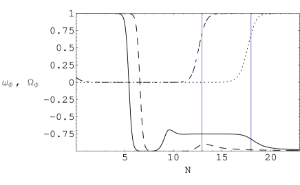
Figure 2: We show the evolution for $\Omega_{\phi},w_{\phi}$ for initial condition $\Omega_{\phi i}=0.07$ dashed-dotted and dashed lines, respectively and for $\Omega_{\phi i}=10^{-10}$, dotted and solid lines, respectively, with $n=2/3$. The first case corresponds to $g_{ex}=64$ while the later case has a huge number of extra degrees of freedom $g_{ex}>10^{9}$. The vertical lines correspond to present day values with $\Omega_{\phi o}=0.7$ and $h_{o}=0.7$.

In this section we study the three different models given in table 1. It is interesting to note that all three models have a one-loop beta function coefficient $b_{o}=3N_{c}-N_{f}=3$ which implies that they have the same condensations scale $\Lambda_{c}=4.2\times 10^{-8}GeV$. The power of the exponent $n$, see table 1, is very similar and if we take the closest integer value for $N_{f}$ one has $n=2/3$ or $6/11$. Notice that model I is self dual $\tilde{N}_{c}=N_{f}-N_{c}=3$ with $N_{f}$ matter fields. The other two models are not self dual.

From now on we will focus on the Model I of table 2 and we will summarize the relevant quantities in table 3 for all models.

The initial energy density at the unification scale is given by eq.(14) with $g_{Qi}=97.5,g_{smi}=228.75$ is $\Omega_{Q}(\Lambda_{gut})=0.3$. Below $\Lambda_{gut}$ the fields are weakly coupled, massless (they redshift as radiation) and are decoupled from the SM. A phase transition takes place when the gauge coupling constant becomes strong at the condensation scale. Since the condensation scale is much smaller than the NS scale, $\Lambda_{c}\ll 0.1MeV$, we expect all fields of the $Q$ group to be relativistic at NS. From eq.(17) with $g_{smf}=10.75$ the energy density, assuming no extra degrees of freedom, is $\Omega_{Q}|_{NS}=0.13$ for susy Model I. In order to satisfy the NS bound $\Omega_{Q}|_{NS}<0.1$, 64 extra relativistic degrees of freedom in thermal equilibrium with the SM at $T\leq T_{gut}$ are required while for $\Omega_{Q}|_{NS}<0.2$ the model does not require any extra degrees of freedom.

What is the energy density of $Q$ at the condensation scale $\Lambda_{c}$? Using eq.(14) with $g_{smf}=3.36,g_{Qf}=97.5$ given at $\Lambda_{c}=4.2\times 10^{-8}GeV$ and with no extra degrees of freedom at the unification scale (i.e. $g_{smi}=228.75$ and $g_{Qi}=g_{Qf}=97.5$) for Model I one has $\Omega_{\phi}(\Lambda_{c})=\Omega_{Q}(\Lambda_{c})=0.095$. Imposing the stringent NS bound $\Omega_{Q}|_{NS}<0.1$ we need to include $g_{ex}=64$ extra degrees of freedom (that should come from susy breaking mechanism) and the energy at $\Lambda_{c}$ is now $\Omega_{\phi}(\Lambda_{c})=0.07$.

Evolving eqs.(4) with initial condition $\Omega_{\phi}(\Lambda_{c})=0.07$ gives at present time with $h_{o}=0.7,\;\Omega_{\phi o}=0.7$ a value of $w_{eff}\equiv\int da\ \Omega(a)w_{\phi}(a)/\int da\ \Omega(a)=-0.93$ with of $w_{\phi o}=-0.90$ in agreement with SN1a and CMBR data. The analytic solution given in eq.(22) is $w_{\phi o}(Th)=-0.82$ and it is a much better approximation to the numerical value then the tracker value $w_{tr}=-2/(2+n)=-0.75$ [10] which is the upper value of $w_{\phi o}$ for given $n$ and arbitrary initial conditions.

From a cosmological evolution point of view, we have a large range of initial condition of $\Omega_{\phi i}$ [27]. The upper limit is set by NS and there is no ”reasonable” lower limit (a smaller $\Omega_{\phi i}$ implies that we have a much larger number of extra degrees of freedom $g_{ex}$ but it must be finite) still gives an acceptable model and there is clearly no fine tuning in these models. The effect of a large number of extra degrees of freedom $g_{ex}\sim 10^{3}$ at the condensation scale is to drop the energy density from $\Omega_{\phi}(\Lambda_{c})=0.07$ with $g_{ex}=64$ to $\Omega_{\phi}(\Lambda_{c})=0.01$ with $g_{ex}=10^{3}$ and the numerical solution, in this case, gives $w_{\phi o}=-0.82$ at present time still within the observational limits. In fact, there is no upper limit for $g_{ex}$ from the cosmological evolution constrains for $\phi$ because the upper value for $w_{\phi o}$ is given by its tracker value which for $n=2/3$ is $w_{tr}=-0.75<-2/3$ smaller than the upper limit given by SN1a and CMBR data. In figure 2 we show the evolution of $\Omega_{\phi},w_{\phi}$ for the minimal number of $g_{ex}=64$ ($\Omega_{\phi i}=0.07$) and for an extreme case with $g_{ex}\sim 10^{9}$ ($\Omega_{\phi i}=10^{-10}$) and in both cases we get an acceptable model.

In table 2 and 3 we summarize the relevant cosmological quantities. In table 2 we give the values of $n,b_{o}$, the degrees of freedom of $Q$ with ($g_{Qs}$) and without supersymmetry ($g_{Qnsusy}$), the condensation scale $\Lambda_{c}$. Notice that all models have same $b_{o},\Lambda_{c}$ but $n$ differs slightly. Model I is the minimal model, in the sense that it has the smallest number of degrees of freedom.

In table 3 we give the values of the initial energy density $\Omega_{Q}(\Lambda_{gut})$, the energy density at NS (for $g_{ex}=0)$, the number of extra degrees of freedom needed to have $\Omega_{Q}(NS)=0.1$ or 0.2, the value of $\Omega_{\phi}(\Lambda_{c})$ with $g_{ex}=0$, the value of $N_{Tot}$ (the e-folds from $\Lambda_{c}$ to present day), the values of $w_{\phi o}$ and $w_{eff}$ calculated numerically and the value obtain analytically from eq.(22) gives a good approximation to the numerical one. The energy density at $\Lambda_{c}$ with the condition $\Omega_{Q}(NS)\leq 0.1$ gives $\Omega_{\Lambda_{c}}=0.07$ for all three models while for $\Omega_{Q}(NS)\leq 0.2$ gives $\Omega_{\Lambda_{c}}=0.15$ for models II and III, respectively. Since the number of $g_{ex}$ for models II and III is quite large (larger than MSSM) we consider them less ”natural” then the minimal Model I.

Num	$N_{c}$	$N_{f}$	$\nu$	$n$	$16\pi^{2}b_{o}$	$\Lambda_{c}(GeV)$	$g_{Qs}$
I	3	6	1	2/3	3	$4.2\times 10^{-8}$	97.5
II	6	15	3	2/3	3	$4.2\times 10^{-8}$	468.5
III	7	18	4	6/11	3	$4.2\times 10^{-8}$	652.5

Table 2: We show the matter content for the three different models and we give the number of degrees of freedom for the susy and non susy $Q$ group in the last two columns, respectively. Notice that the condensation scale and $b_{o}$ is the same for all models.

Num	$\Omega_{Q}(\Lambda_{gut})$	$\Omega_{Q}(NS)$	$\Omega_{\phi}(\Lambda_{c})$	$g_{ex1}$	$g_{ex2}$	$w_{\phi o}$	$w_{eff}$	$w_{\phi o}(Th)$	$N_{Tot}$
I	0.30	0.13	0.09	64	0	-0.90	-0.93	-0.82	12.9
II	0.67	0.42	0.33	718	287	-0.90	-0.93	-0.82	12.9
III	0.74	0.50	0.41	986	433	-0.93	-0.95	-0.87	11.1

Table 3: The first column gives the model number. In columns 2-4 we give the energy density at different scales assuming no extra degrees of freedom (i.e. $g_{ex}=0$). In column 5 and 6 we show the necessary number of $g_{ex}$ to have $\Omega_{Q}(NS)\leq 0.1,0.2$, respectively. We show in columns 7, 8 the present day value of $w_{\phi}$ calculated numerically and in column 9 the theoretically obtained from eq.(22). Finally, we give in the last column the number of e-folds of expansion from $\Lambda_{c}$ to present day.

6 Summary and Conclusions

We have shown that an unification scheme, where all coupling constants are unified, as predicted by string theory, leads to an acceptable cosmological constant parameterized in terms of the condensates of a non-abelian gauge group. These fields play the role of quintessence.

Above the unification scale we have all fields in thermal equilibrium and the number of degrees of freedom for the SM and $Q$ model determines the initial conditions for each group. Below $\Lambda_{gut}$ the $Q$ group decouples, since it interacts with the SM only through gravity. For temperatures above the condensation scale of the $Q$ group its fields are relativistic and red shift as radiation. The entropy of each systems is independently conserved and we can therefore determine the energy density at NS and at $\Lambda_{c}$. The models we have obtain have a condensation scale below NS and in order not to spoil the NS predictions the energy density must be $\Omega_{Q}(NS)<0.1-0.2$.

Without considering the contribution from the susy breaking sector, all models have $\Omega_{Q}>0.1$ with the smallest contribution from Model I ($N_{c}=3,N_{f}=6$ minimal model) giving $\Omega_{Q}=0.13$ in agreement with the conservative bound $\Omega_{Q}|_{NS}<0.2$ NS bound and slightly large then $\Omega_{Q}|_{NS}<0.1$. If susy is transmitted via gravity we require extra structure to agree with the strongest NS (the gauge group responsible for susy breaking is not in thermal equilibrium with the SM below $\Lambda_{gut}$) but if susy is gauge mediated than the NS bound is alleviated since one has extra degrees of freedom $g_{ex}$ in thermal equilibrium with the SM. The cosmological evolution of quintessence is not sensitive to the number of the extra degrees of freedom. There is a minimum number required from NS bounds but there is no upper limit.

At the condensation scale the $Q$ fields are no longer free and they condense. We use Affleck’s potential to parameterize the condensates and we study the cosmological evolution with the initial condition determined in terms of $N_{c},N_{f}$ only. Gauge unification determines the values of $N_{c},N_{f}$ and there are no models with $2\times 10^{-2}GeV<\Lambda_{c}<6\times 10^{3}GeV$ or $2<n<4.27$. Since $w_{\phi o}<-2/3$ requires $n<2.74$ all models must have $\Lambda_{c}>2\times 10^{-2}GeV$ or $n>2$. The three acceptable models have a potential of the form $V\sim\phi^{-n}$ with $6/11\leq n\leq 2/3$. The value of $n$ and the energy density at $\Lambda_{c}$ determines the present day value of $w_{\phi o}$. We show that the models have $\Omega_{\phi o}=0.7,w_{\phi o}=-0.90$ with a Hubble parameter $h_{o}=0.7$ and the value of $n$ and $w_{\phi o}$ are in accordance with constrains from recent CMBR analysis, i.e. $n<1$ and $w_{\phi o}=-0.82^{+.14}_{-.11}$ [7, 8]. We also show that the tracker solution to inverse power potential is not specific enough (in Model I $w_{tr}=-0.75$) and does not give a good approximation for models with $n<2$, which are the cosmologically favored.

We would like to stress out that there are no free parameters, not even the $Q$ initial energy density at unification nor at the condensation scale. The models are well motivated from a particle physics point of view, they involve a late time phase transition, and they agree with present day observations.

This work was supported in part by CONACYT project 32415-E and DGAPA, UNAM project IN-110200.

References

- [1]
- [2]
- [3] P. de Bernardis et al. Nature, (London) 404, (2000) 955, S. Hannany et al.,Astrophys.J.545 (2000) L1-L4
- [4] A.G. Riess et al., Astron. J. 116 (1998) 1009; S. Perlmutter et al, ApJ 517 (1999) 565; P.M. Garnavich et al, Ap.J 509 (1998) 74.
- [5] G. Efstathiou, S. Maddox and W. Sutherland, Nature 348 (1990) 705. J. Primack and A. Klypin, Nucl. Phys. Proc. Suppl. 51 B, (1996), 30
- [6] S. Perlmutter, M. Turner and M. J. White, Phys.Rev.Lett.83:670-673, 1999; T. Saini, S. Raychaudhury, V. Sahni and A.A. Starobinsky, Phys.Rev.Lett.85:1162-1165,2000
- [7] Carlo Baccigalupi, Amedeo Balbi, Sabino Matarrese, Francesca Perrotta, Nicola Vittorio, astro-ph/0109097
- [8] Michael Doran, Matthew J. Lilley, Jan Schwindt, Christof Wetterich, astro-ph/0012139; Michael Doran, Matthew Lilley, Christof Wetterich astro-ph/0105457
- [9] P.S. Corasaniti, E.J. Copeland, astro-ph/0107378
- [10] I. Zlatev, L. Wang and P.J. Steinhardt, Phys. Rev. Lett.82 (1999) 8960; Phys. Rev. D59 (1999)123504
- [11] P.J.E. Peebles and B. Ratra, ApJ 325 (1988) L17; Phys. Rev. D37 (1988) 3406
- [12] J.P. Uzan, Phys.Rev.D59:123510,1999
- [13] P. Binetruy, Phys.Rev. D60 (1999) 063502, Int. J.Theor. Phys.39 (2000) 1859
- [14] A. Masiero, M. Pietroni and F. Rosati, Phys. Rev. D61 (2000) 023509
- [15] A. de la Macorra and C. Stephan-Otto, Phys.Rev.Lett.87:271301,2001
- [16] A.R. Liddle and R.J. Scherrer, Phys.Rev. D59, (1999)023509
- [17] A. de la Macorra and G. Piccinelli, Phys. Rev.D61 (2000) 123503
- [18] E.J. Copeland, A. Liddle and D. Wands, Phys. Rev. D57 (1998) 4686
- [19] P. Brax, J. Martin, Phys.Rev.D61:103502,2000
- [20] E.Kolb and M.S Turner,The Early Universe, Edit. Addison Wesley 1990
- [21] K. Freese, F.C. Adams, J.A. Frieman and E. Mottola, Nucl. Phys. B 287 (1987) 797; M. Birkel and S. Sarkar, Astropart. Phys. 6 (1997) 197.
- [22] C. Wetterich, Nucl. Phys. B302 (1988) 302, R.H. Cyburt, B.D. Fields, K. A. Olive, Astropart.Phys.17:87-100,2002
- [23] I. Affleck, M. Dine and N. Seiberg, Nucl. Phys.B256 (1985) 557
- [24] M.A. Shifman and A.I. Vainshtein, Nucl. Phys. B277 (1986) 649
- [25] C.P. Burgess, A. de la Macorra, I. Maksymyk and F. Quevedo Phys.Lett.B410 (1997) 181
- [26] A. de la Macorra, Int.J.Mod.Phys.D9 (2000) 661
- [27] A. de la Macorra and C. Stephan-Otto, Phys.Rev.D65:083520,2002
- [28] U. Amaldi, W. de Boer and H. Furstenau, Phys. Lett.B260 (1991) 447, P.Langacker and M. Luo, Phys. Rev.D44 (1991) 817
- [29]
- [30] K. Intriligator and N. Seiberg, Nucl.Phys.Proc.Suppl.45BC:1-28,1996
- [31] M. Dine, R. Rhom, N. Seiberg and E. Witten, Phys. Lett. B156 (1985) 55, G. Veneziano and S. Yankielowicz, Phys. Lett. B113 (1984)231; S. Ferrara, L. Girardello and H.P. Nilles, Phys. Lett. B125 (1983) 457, D. Amati, K. Konishi, Y. Meurice, G. Rossi and G. Veneziano, Phys. Rep. 162 (1988) 169
- [32] T.R. Taylor, Phys.Lett.B252 (1990) 59;H. P. Nilles Int.J.Mod.Phys.A5 (1990) 4199; B. de Carlos, J.A. Casas, C. Munoz, Nucl.Phys.B399 (1993) 623; M. Cvetic, A. Font, Luis E. Ibanez, D. Lust), F. Quevedo Nucl.Phys.B361 (1991) 194, Phys.Lett.B245 (1990) 401; A. de la Macorra and G.G. Ross, Phys. Lett. B Nucl.Phys.B404 (1993) 321, Nucl.Phys.B443 (1995)127-154
- [33] G.F. Giudice, R. Rattazzi, Phys.Rept.322:(1999) 419-499 and ref. therein