On the Mixed Propagator Approach to $\rho-\omega$ Mixing ††thanks: This work is partly supported by the grant No.90103002 of National Natural Science Foundation of China.

Mu-Lin Yan***mlyan@ustc.edu.cn, Ji-Hao Jiang    Xiao-Jun Wang
Abstract

Mixed Propagator (MP) approach to $\rho-\omega$ mixing is discussed. It is found that under the pole-approximation assumption the results of MP approach is not compatible both with the effective Lagrangian theory and with the experiment measurement criterion. To overcome these inconsistent, we propose a new MP approach in which the physical states of $\rho$ and $\omega$ are determined by the requirement of experimental measurement to meson resonance. In terms of this new MP approach, the EM pion form factor $F_{\pi}$ and form factors of $\rho^{0}\rightarrow\pi^{0}\gamma$ and of $\omega\rightarrow\pi^{0}\gamma$ are derived. The results of $F_{\pi}$ are in good agreement with data. The form factor of $\rho^{0}\rightarrow\pi^{0}\gamma$ exhibits a hidden charge-asymmetry enhancement effect which agree with the prediction of the effective Lagrangian theory.

14.40.Cs,13.25.Jx,12.40.Vv,13.40.Hq

$\rho^{0}-\omega$ mixing (or $\rho^{0}-\omega$ interference, or interference between overlapping resonances, or charge asymmetry caused by $\rho-\omega$ mixing and so on) has attracted much interest during past four decades. Since 1961[1], there is a great deal of works on this subject in the literature (see, for example, review articles[2, 3] and the references within). Recently, we used model-independent effective Lagrangian (eff-L) approach to discuss $\rho-$ and $\omega-$ anomaly-like processes of $\rho^{0}\rightarrow\pi^{0}\gamma$, and of $\omega\rightarrow\pi^{0}\gamma$[4]. It has been found that there exist a hidden charge-asymmetry enhancement effect to $\rho^{0}\rightarrow\pi^{0}\gamma$ due to $\rho^{0}-\omega$ mixing. Namely, we have (by using the notations in ref[4])

$\displaystyle f_{\rho^{0}\pi^{0}\gamma}|_{\rm eff-L}$ $\displaystyle=$ fρ0​π0​γ(0)​(1+3​Πρ​ω​(mρ2)mρ2βˆ’mΟ‰2+i​mω​Γω),subscriptsuperscript𝑓0superscript𝜌0superscriptπœ‹0𝛾13subscriptΞ πœŒπœ”superscriptsubscriptπ‘šπœŒ2superscriptsubscriptπ‘šπœŒ2superscriptsubscriptπ‘šπœ”2𝑖subscriptπ‘šπœ”subscriptΞ“πœ”\displaystyle f^{(0)}_{\rho^{0}\pi^{0}\gamma}(1+\frac{3\Pi_{\rho\omega}(m_{\rho}^{2})}{m_{\rho}^{2}-m_{\omega}^{2}+im_{\omega}\Gamma_{\omega}}), (1)
$\displaystyle f_{\omega\pi^{0}\gamma}|_{\rm eff-L}$ $\displaystyle=$ fω​π0​γ(0)​(1+13​Πρ​ω​(mΟ‰2)mΟ‰2βˆ’mρ2+i​mρ​Γρ),subscriptsuperscript𝑓0πœ”superscriptπœ‹0𝛾113subscriptΞ πœŒπœ”superscriptsubscriptπ‘šπœ”2superscriptsubscriptπ‘šπœ”2superscriptsubscriptπ‘šπœŒ2𝑖subscriptπ‘šπœŒsubscriptΞ“πœŒ\displaystyle f^{(0)}_{\omega\pi^{0}\gamma}(1+{1\over 3}\frac{\Pi_{\rho\omega}(m_{\omega}^{2})}{m_{\omega}^{2}-m_{\rho}^{2}+im_{\rho}\Gamma_{\rho}}), (2)

where the subscript ’eff-L’ means the results obtained by in the effective Lagrangian approach. Due to $\Gamma_{\omega}<<\Gamma_{\rho}$, we have

$\displaystyle|f_{\rho^{0}\pi^{0}\gamma}|_{\rm eff-L}$ $\displaystyle>>$ $\displaystyle f^{(0)}_{\rho^{0}\pi^{0}\gamma}=f_{\rho^{\pm}\pi^{\pm}\gamma}$ (3)
$\displaystyle|f_{\omega\pi^{0}\gamma}|_{\rm eff-L}$ $\displaystyle\sim$ $\displaystyle f^{(0)}_{\omega\pi^{0}\gamma}.$ (4)

This reflects an unusual charge asymmetry enhancement effect for $\rho\rightarrow\pi\gamma$. As addressed in[4], this hidden effect has already been implied by experiment[5].

On the other hand, There is a well-known quantum mechanics method to deal with the $\rho-\omega$ mixing problem: the approach of mixed propagator with pole approximation (shortly, we will call it as pole-Mixed-Propagator approach, or pole-MP approach)[2, 3]. This approach was developed even before discovery of QCD. A question arisen here what are results for $\rho^{0}\rightarrow\pi^{0}\gamma$ and $\omega\rightarrow\pi^{0}\gamma$ in pole-MP approach? The vector meson propagator is given by (Renard representation)

$\displaystyle D_{\mu\nu}(q^{2})$ $\displaystyle=$ $\displaystyle\int d^{4}xe^{-iq.x}\langle 0|T\{V_{\mu}(x)V_{\nu}(0)\}|0\rangle$ (5)
$\displaystyle=$ $\displaystyle D(q^{2})g_{\mu\nu}+{1\over q^{2}}(D(0)-D(s))q_{\mu}q_{\nu}$ (6)

where $s\equiv q^{2}$, and the propagator function $D(s)$ is written in the following way

D​(s)=1sβˆ’W​(s).𝐷𝑠1π‘ π‘Šπ‘ D(s)={1\over s-W(s)}. (7)

For multi-vector-meson channels, W​(s)π‘Šπ‘ W(s) is complex mass-square matrix with non-zero off-diagonal elements in general. The basic assumption for pole-MP approach is that the physical states are eigenvectors of W​(s)π‘Šπ‘ W(s), or the complex mass-square of physical state is determined by the following equation

d​e​t​[sβˆ’W​(s)]=0.𝑑𝑒𝑑delimited-[]π‘ π‘Šπ‘ 0det[s-W(s)]=0. (8)

For $\rho-\omega$ case, the solutions of this physical condition equation are follows[3]

$\displaystyle|\rho_{p}^{0}\rangle$ $\displaystyle=$ $\displaystyle|\rho_{I}^{0}\rangle+\epsilon|\omega_{I}\rangle,\;\;\langle\tilde{\rho}^{0}_{p}|=\langle\rho_{I}^{0}|-\epsilon\langle\omega_{I}|$ (9)
$\displaystyle|\omega_{p}\rangle$ $\displaystyle=$ $\displaystyle|\omega_{I}\rangle-\epsilon|\rho_{I}^{0}\rangle,\;\;\langle\tilde{\omega}_{p}|=\langle\omega_{I}^{0}|+\epsilon\langle\rho^{0}_{I}|$ (10)

with

Ο΅=Πρ​ωmΟ‰2βˆ’mρ2+i​(mΟ‰β€‹Ξ“Ο‰βˆ’mρ​Γρ),italic-Ο΅subscriptΞ πœŒπœ”superscriptsubscriptπ‘šπœ”2superscriptsubscriptπ‘šπœŒ2𝑖subscriptπ‘šπœ”subscriptΞ“πœ”subscriptπ‘šπœŒsubscriptΞ“πœŒ\epsilon={\Pi_{\rho\omega}\over m_{\omega}^{2}-m_{\rho}^{2}+i(m_{\omega}\Gamma_{\omega}-m_{\rho}\Gamma_{\rho})}, (11)

where $|\rho_{p}^{0}\rangle$ and $|\omega_{p}\rangle$ denote physical $\rho^{0}-$ and $\omega-$ states under the pole approximation assumption respectively, $|\rho_{I}^{0}\rangle\equiv|1,0\rangle$ and $|\omega_{I}\rangle\equiv|0,0\rangle$ are in the isospin basis, and Ξ Οβ€‹Ο‰β‰‘βŸ¨ΟI0|W|Ο‰I⟩subscriptΞ πœŒπœ”quantum-operator-productsuperscriptsubscript𝜌𝐼0π‘Šsubscriptπœ”πΌ\Pi_{\rho\omega}\equiv\langle\rho_{I}^{0}|W|\omega_{I}\rangle. Note that $\epsilon$ is not a real number, and hence the transfer matrix from isospin basis to physical basis is not unitary. The physical states are normalized in following way

$$\langle\tilde{a}|b\rangle=\delta_{ab}\;\;\;{\rm and}\;\;\;\;{\bf I}=\sum_{a}|\tilde{a}\rangle\langle a|=\sum_{a}|{a}\rangle\langle\tilde{a}|$$ (12)

where $a,\;b=\rho^{0}_{p}$ or $\omega_{p}$. Because the transfer matrix between the isospin bases and the physical one is not unitary in the pole-MP, the relations of eq.Β (9) can not be realized in the formalism of unitary Lagrangian field theory. Since it has been widely accepted that the effective Lagrangian field theories inspired by QCD conceptions (e.g., VMD, large $N_{c}$ expansion, non-linear realization of chiral symmetry, WCCWZ realization, WZ-anomaly, hidden local symmetry and so on) is legitimate and useful to study $\rho-$ and $\omega-$ physics[6], that the pole-MP approach contradicts to effective Lagrangian field theory is a difficulty for pole-MP.

To show the differences between two approach further, let us consider $\rho^{0},\omega\to\pi^{0}\gamma$ decays in the pole-MP. Again, using $f_{\rho^{0}\pi^{0}\gamma},\;f_{\omega\pi^{0}\gamma}$ and $f^{(0)}_{\rho^{0}\pi^{0}\gamma},\;f^{(0)}_{\omega\pi^{0}\gamma}$ to denote the physical coupling constants and the isospin-basis constants respectively, we have

$\displaystyle f_{\rho^{0}\pi^{0}\gamma}|_{\rm pole-MP}$ $\displaystyle=$ fρ0​π0​γ(0)​(1+3​Πρ​ω​(mρ2)mρ2βˆ’mΟ‰2+i​(mΟ‰β€‹Ξ“Ο‰βˆ’mρ​Γρ)),subscriptsuperscript𝑓0superscript𝜌0superscriptπœ‹0𝛾13subscriptΞ πœŒπœ”superscriptsubscriptπ‘šπœŒ2superscriptsubscriptπ‘šπœŒ2superscriptsubscriptπ‘šπœ”2𝑖subscriptπ‘šπœ”subscriptΞ“πœ”subscriptπ‘šπœŒsubscriptΞ“πœŒ\displaystyle f^{(0)}_{\rho^{0}\pi^{0}\gamma}(1+\frac{3\Pi_{\rho\omega}(m_{\rho}^{2})}{m_{\rho}^{2}-m_{\omega}^{2}+i(m_{\omega}\Gamma_{\omega}-m_{\rho}\Gamma_{\rho})}), (13)
$\displaystyle f_{\omega\pi^{0}\gamma}|_{\rm pole-MP}$ $\displaystyle=$ fω​π0​γ(0)​(1+13​Πρ​ω​(mΟ‰2)mΟ‰2βˆ’mρ2βˆ’i​(mΟ‰β€‹Ξ“Ο‰βˆ’mρ​Γρ)).subscriptsuperscript𝑓0πœ”superscriptπœ‹0𝛾113subscriptΞ πœŒπœ”superscriptsubscriptπ‘šπœ”2superscriptsubscriptπ‘šπœ”2superscriptsubscriptπ‘šπœŒ2𝑖subscriptπ‘šπœ”subscriptΞ“πœ”subscriptπ‘šπœŒsubscriptΞ“πœŒ\displaystyle f^{(0)}_{\omega\pi^{0}\gamma}(1+{1\over 3}\frac{\Pi_{\rho\omega}(m_{\omega}^{2})}{m_{\omega}^{2}-m_{\rho}^{2}-i(m_{\omega}\Gamma_{\omega}-m_{\rho}\Gamma_{\rho})}). (14)

where $f^{(0)}_{\omega\pi^{0}\gamma}=3f^{(0)}_{\rho^{0}\pi^{0}\gamma}$ has been used. Comparing eq.Β (1) with eq.Β (13) and noting $\Gamma_{\omega}<<\Gamma_{\rho}$, we can see

$\displaystyle f_{\rho^{0}\pi^{0}\gamma}|_{\rm pole-MP}$ $\displaystyle\sim$ $\displaystyle f^{(0)}_{\rho^{0}\pi^{0}\gamma}<<f_{\rho^{0}\pi^{0}\gamma}|_{\rm eff-L}$ (15)
$\displaystyle f_{\omega\pi^{0}\gamma}|_{\rm pole-MP}$ $\displaystyle\sim$ $\displaystyle f^{(0)}_{\omega\pi^{0}\gamma}\sim f_{\omega\pi^{0}\gamma}|_{\rm eff-L}$ (16)

Eq.Β (15) indicates there is no the hidden charge-asymmetry enhancement effect for $\rho^{0}\rightarrow\pi^{0}\gamma$ mentioned above in the pole-MP formalism. The result of pole-MP approach to $\rho^{0}\rightarrow\pi^{0}\gamma$ is significantly different from one of eff-L. Thus we learned that there may be something wrong. The purpose of this letter is to re-examine the pole-Mixed Propagator approach, and propose a new mixed propagator approach based on the criterion of experimental measurement to meson resonances.

Let’s consider whether the pole-MP assumption on physical states eq.Β (8) is consistent with the experimental criterion to measure the physical meson resonance or not. We first consider the single vector meson resonance channel case. The $D_{\mu\nu}$ of eq.Β (5) is now the ordinary propagator of a vector meson. The reaction amplitude for a process by the medium of this vector meson resonance reads

β„³βˆΌJ1μ​Dμ​ν​J2Ξ½=(J1β‹…J2)​1sβˆ’W​(s)similar-toβ„³superscriptsubscript𝐽1πœ‡subscriptπ·πœ‡πœˆsuperscriptsubscript𝐽2πœˆβ‹…subscript𝐽1subscript𝐽21π‘ π‘Šπ‘ {\cal M}\sim J_{1}^{\mu}D_{\mu\nu}J_{2}^{\nu}=(J_{1}\cdot J_{2}){1\over s-W(s)} (17)

where $J_{1}^{\mu}$ and $J_{2}^{\nu}$ represent some currents and $q_{\mu}J_{1,\;2}^{\mu}=0$. The reaction probability is[8]

σ​(s)∼|β„³|2∝|1sβˆ’W​(s)|2similar-toπœŽπ‘ superscriptβ„³2proportional-tosuperscript1π‘ π‘Šπ‘ 2\sigma(s)\sim|{\cal M}|^{2}\propto|{1\over s-W(s)}|^{2} (18)

The meson resonance mass measured in the experiment is real and is determined by the location of the maximum of σ​(s)βˆ’limit-fromπœŽπ‘ \sigma(s)-peak in real $s-$axis. Then the resonance mass is determined by the following equation

βˆ‚βˆ‚s​|sβˆ’W​(s)|2=0𝑠superscriptπ‘ π‘Šπ‘ 20{\partial\over\partial s}|{s-W(s)}|^{2}=0 (19)

Consequently, the mass-square of the resonance, $M^{2}$, is determined by the solution of above equation, i.e.,

s=[R​e​Wβˆ’14β€‹βˆ‚βˆ‚s​(Wβˆ—β€‹W+W​Wβˆ—)]​(1βˆ’βˆ‚βˆ‚s​R​e​W)βˆ’1≑M2​(s).𝑠delimited-[]π‘…π‘’π‘Š14𝑠superscriptπ‘Šπ‘Šπ‘Šsuperscriptπ‘Šsuperscript1π‘ π‘…π‘’π‘Š1superscript𝑀2𝑠s=[ReW-{1\over 4}{\partial\over\partial s}(W^{*}W+WW^{*})](1-{\partial\over\partial s}ReW)^{-1}\equiv M^{2}(s). (20)

Now return to $\rho^{0}-\omega$ two channel case, W​(s)π‘Šπ‘ W(s) and hence $M^{2}(s)$ are $2\times 2$ matrices. The mass determination equation for physical resonance states should read

$$det[s-M^{2}(s)]=0.$$ (21)

The physical states then are the eigenvectors of the real mass-matrix $M^{2}$. Obviously, the corresponding pole-MP equationΒ (8) is definitely different from above mass determination equation derived from the experiment measurement principle to physical resonance states. It indicates that the the pole-MP is not consistent with the criterion of experimental measurement to the physical resonances. Consequently, we should use eq.Β (21) to define true physical $\rho-$ and $\omega-$fields, and rule out the condition of eq.Β (8). For convenience, we will call this method hereafter as Experiment-criterion Mixed Propagator approach, or expt-MP approach.

Now let us use expt-MP to fit experiments. Following refs[2, 3] and using Breit-Wigner approximation, we have

W=(mρI2βˆ’i​s​ΓρIΠρ​ω​(s)Πρ​ω​(s)mΟ‰I2βˆ’i​s​ΓωI)π‘Šsuperscriptsubscriptπ‘šsubscript𝜌𝐼2𝑖𝑠subscriptΞ“subscript𝜌𝐼subscriptΞ πœŒπœ”π‘ missing-subexpressionsubscriptΞ πœŒπœ”π‘ superscriptsubscriptπ‘šsubscriptπœ”πΌ2𝑖𝑠subscriptΞ“subscriptπœ”πΌmissing-subexpression\displaystyle W=\left(\begin{array}[]{lcr}m_{\rho_{I}}^{2}-i\sqrt{s}\Gamma_{\rho_{I}}&\Pi_{\rho\omega}(s)\\ \Pi_{\rho\omega}(s)&m_{\omega_{I}}^{2}-i\sqrt{s}\Gamma_{\omega_{I}}\end{array}\right) (24)

Considering ImΠρ​ωsubscriptΞ πœŒπœ”\Pi_{\rho\omega} is small and hence ignorable[9], we get

R​e​W=(mρI2Πρ​ω​(s)Πρ​ω​(s)mΟ‰I2)π‘…π‘’π‘Šsuperscriptsubscriptπ‘šsubscript𝜌𝐼2subscriptΞ πœŒπœ”π‘ missing-subexpressionsubscriptΞ πœŒπœ”π‘ superscriptsubscriptπ‘šsubscriptπœ”πΌ2missing-subexpression\displaystyle ReW=\left(\begin{array}[]{lcr}m_{\rho_{I}}^{2}&\Pi_{\rho\omega}(s)\\ \Pi_{\rho\omega}(s)&m_{\omega_{I}}^{2}\end{array}\right) (27)

Then, in βˆ‚R​e​W/βˆ‚sπ‘…π‘’π‘Šπ‘ \partial ReW/\partial s, only off-diagonal elements of βˆ‚Ξ Οβ€‹Ο‰/βˆ‚ssubscriptΞ πœŒπœ”π‘ {\partial\Pi_{\rho\omega}/\partial s} is left. Generally, for a broad class of models Πρ​ω​(s)subscriptΞ πœŒπœ”π‘ \Pi_{\rho\omega}(s) at $(\rho-,\omega-)$resonance energy region can be determined by taking VMD-type $\rho-\omega$ mixing Lagrangian ${\cal L}_{\rho\omega}=f_{\rho\omega}\rho^{\mu\nu}\omega_{\mu\nu}$ ( $V^{\mu\nu}=\partial^{\mu}V^{\nu}-\partial^{\nu}V^{\mu},\ V=\rho,\omega$). It leads to Πρ​ω​(s)=fρ​ω​ssubscriptΞ πœŒπœ”π‘ subscriptπ‘“πœŒπœ”π‘ \Pi_{\rho\omega}(s)=f_{\rho\omega}s which satisfies Π​(s=0)ρ​ω=0Ξ subscript𝑠0πœŒπœ”0\Pi(s=0)_{\rho\omega}=0 required by generic consideration in ref[10]. Thus, we have

βˆ‚βˆ‚s​Πρ​ω=fρ​ω=Πρ​ωs|s∼mρ2≃6.7Γ—10βˆ’3β‰ͺ1⟹ 1βˆ’(βˆ‚R​e​W/βˆ‚s)≃1.𝑠subscriptΞ πœŒπœ”subscriptπ‘“πœŒπœ”evaluated-atsubscriptΞ πœŒπœ”π‘ similar-to𝑠subscriptsuperscriptπ‘š2𝜌similar-to-or-equals6.7superscript103much-less-than1⟹1π‘…π‘’π‘Šπ‘ similar-to-or-equals1{\partial\over{\partial s}}\Pi_{\rho\omega}=f_{\rho\omega}={\Pi_{\rho\omega}\over s}|_{s\sim m^{2}_{\rho}}\simeq 6.7\times 10^{-3}\ll 1\ \Longrightarrow\ 1-({\partial ReW}/{\partial s})\simeq 1. (28)

where |Πρ​ω|≃4000​M​e​V2similar-to-or-equalssubscriptΞ πœŒπœ”4000𝑀𝑒superscript𝑉2|\Pi_{\rho\omega}|\simeq 4000MeV^{2}[10] has been used in the estimation. Furthermore, noting $\Gamma_{\omega}/m_{\omega}\ll 1$, we have

M2=(mρI2βˆ’βˆ‚(s​Γρ2)βˆ‚sΞ Οβ€‹Ο‰βˆ’12​(mρI2+mΟ‰I2)β€‹βˆ‚βˆ‚sβ€‹Ξ Οβ€‹Ο‰Ξ Οβ€‹Ο‰βˆ’12​(mρI2+mΟ‰I2)β€‹βˆ‚βˆ‚s​Πρ​ωmΟ‰I2)superscript𝑀2superscriptsubscriptπ‘šsubscript𝜌𝐼2𝑠superscriptsubscriptΞ“πœŒ2𝑠subscriptΞ πœŒπœ”12superscriptsubscriptπ‘šsubscript𝜌𝐼2superscriptsubscriptπ‘šsubscriptπœ”πΌ2𝑠subscriptΞ πœŒπœ”subscriptΞ πœŒπœ”12superscriptsubscriptπ‘šsubscript𝜌𝐼2superscriptsubscriptπ‘šsubscriptπœ”πΌ2𝑠subscriptΞ πœŒπœ”superscriptsubscriptπ‘šsubscriptπœ”πΌ2\displaystyle M^{2}=\left(\begin{array}[]{cc}m_{\rho_{I}}^{2}-{\partial(s\Gamma_{\rho}^{2})\over\partial s}&\Pi_{\rho\omega}-{1\over 2}(m_{\rho_{I}}^{2}+m_{\omega_{I}}^{2}){\partial\over\partial s}\Pi_{\rho\omega}\\ \Pi_{\rho\omega}-{1\over 2}(m_{\rho_{I}}^{2}+m_{\omega_{I}}^{2}){\partial\over\partial s}\Pi_{\rho\omega}&m_{\omega_{I}}^{2}\end{array}\right) (31)

where the off-diagonal elements of $M^{2}$ matrix represent the $\rho-\omega$ mixing in the isospin basis. The physical $\rho$ and $\omega$ are eigenstates of $M^{2}$. Because $M^{2}$ matrix is real and symmetric, distinguishing from the transformation from isospin basis to physical basis in the pole-MP, the corresponding transfer-matrix of expt-MP is unitary. $M^{2}$ matrix is diagonalized by the unitary $2\times 2$ matrix $C$:

$\displaystyle CM^{2}C^{\dagger}=\left(\begin{array}[]{lcr}m_{\rho}^{2}&0\\ 0&m_{\omega}^{2}\end{array}\right)$ (34)

where

C=(1βˆ’Ξ·Ξ·1),Ξ·=βˆ’Ξ Οβ€‹Ο‰β€‹(1βˆ’12​s​(mρ2+mΟ‰2))(mΟ‰2βˆ’mρ2).formulae-sequence𝐢1πœ‚missing-subexpressionπœ‚1missing-subexpressionπœ‚subscriptΞ πœŒπœ”112𝑠superscriptsubscriptπ‘šπœŒ2superscriptsubscriptπ‘šπœ”2superscriptsubscriptπ‘šπœ”2superscriptsubscriptπ‘šπœŒ2\displaystyle C=\left(\begin{array}[]{lcr}1&-\eta\\ \eta&1\end{array}\right),\hskip 36.135pt\eta=-{\Pi_{\rho\omega}(1-{1\over 2s}(m_{\rho}^{2}+m_{\omega}^{2}))\over(m_{\omega}^{2}-m_{\rho}^{2})}. (37)

Consequently, the solutions of expt-MP’s physical state condition of eq.Β (21) are follows

$\displaystyle|\rho_{p}^{0}\rangle$ $\displaystyle=$ |ρI0βŸ©βˆ’Ξ·β€‹|Ο‰I⟩,⟨ρp0|=|ρp0βŸ©β€ ketsuperscriptsubscript𝜌𝐼0πœ‚ketsubscriptπœ”πΌbrasubscriptsuperscript𝜌0𝑝superscriptketsuperscriptsubscriptπœŒπ‘0†\displaystyle|\rho_{I}^{0}\rangle-\eta|\omega_{I}\rangle,\;\;\langle{\rho}^{0}_{p}|=|\rho_{p}^{0}\rangle^{\dagger} (38)
$\displaystyle|\omega_{p}\rangle$ $\displaystyle=$ |Ο‰I⟩+η​|ρI0⟩,βŸ¨Ο‰p|=|Ο‰pβŸ©β€ .ketsubscriptπœ”πΌπœ‚ketsuperscriptsubscript𝜌𝐼0brasubscriptπœ”π‘superscriptketsubscriptπœ”π‘β€ \displaystyle|\omega_{I}\rangle+\eta|\rho_{I}^{0}\rangle,\;\;\langle\omega_{p}|=|\omega_{p}\rangle^{\dagger}. (39)

Under this transformation, we have

C​W​Cβ€ πΆπ‘Šsuperscript𝐢†\displaystyle CWC^{{\dagger}} $\displaystyle=$ $\displaystyle\left(\begin{array}[]{lcr}z_{\rho}&T\\ T&z_{\omega}\end{array}\right)$ (42)

where $z_{\rho}=m_{\rho}^{2}-im_{\rho}\Gamma_{\rho},z_{\omega}=m_{\omega}^{2}-im_{\omega}\Gamma_{\omega}$, and T=Ξ Οβ€‹Ο‰βˆ’Ξ·β€‹(zΟ‰βˆ’zρ)𝑇subscriptΞ πœŒπœ”πœ‚subscriptπ‘§πœ”subscriptπ‘§πœŒT=\Pi_{\rho\omega}-\eta(z_{\omega}-z_{\rho}) are all defined in the physical state basis of expt-MP. The propagator function in the physical basis $D^{P}$ reads

$\displaystyle D^{P}(s)$ $\displaystyle=$ C​(sβˆ’W)βˆ’1​C†=(sβˆ’C​W​C†)βˆ’1𝐢superscriptπ‘ π‘Š1superscript𝐢†superscriptπ‘ πΆπ‘Šsuperscript𝐢†1\displaystyle C(s-W)^{-1}C^{{\dagger}}=(s-CWC^{{\dagger}})^{-1} (43)
$\displaystyle=$ $\displaystyle\left(\begin{array}[]{lcr}(s-z_{\rho})^{-1}&(s-z_{\rho})^{-1}T(s-z_{\omega})^{-1}\\ (s-z_{\omega})^{-1}T(s-z_{\rho})^{-1}&(s-z_{\omega})^{-1}\end{array}\right)$ (46)
$\displaystyle\equiv$ $\displaystyle\left(\begin{array}[]{lcr}D^{P}_{\rho\rho}&D^{P}_{\rho\rho}TD^{P}_{\omega\omega}\\ D^{P}_{\omega\omega}TD^{P}_{\rho\rho}&D^{P}_{\omega\omega}\end{array}\right)\equiv\left(\begin{array}[]{lcr}D^{P}_{\rho\rho}&D^{P}_{\rho\omega}\\ D^{P}_{\omega\rho}&D^{P}_{\omega\omega}\end{array}\right).$ (51)

For $V-X$-vertex ($V=\rho,\;\omega$ and $X$ represents other particles), $f^{F}_{VX}$ denotes the corresponding form-factor, $f^{P}_{VX}$ and $f^{0}_{VX}$ denote the coupling constants in the physical basis and in the isospin basis respectively.

Refer to caption


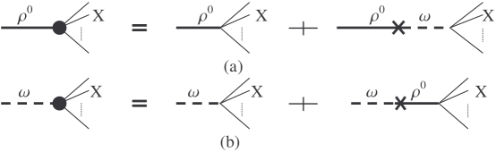
FIG. 1.: The relation between the form factor of $V-X$ vertex and the corresponding coupling constants for the vertices, where $V=\rho$ in Fig.(a) and $V=\omega$ in Fig.(b). In the left-hand side, the black dots in the vertex represent the form factor. In the right-hand side, the coupling constants are at the vertices. The single thick (dash) lines denote for $\rho-$propagator $D^{P}_{\rho\rho}$ ($\omega-$propagator $D^{P}_{\omega\omega}$), and the thick-cross-dash lines (or dash-cross-thick) line denote the mixed propagator $D^{P}_{\rho\omega}$ (or $D^{P}_{\omega\rho}$). The thin lines are external lines of $X$-particles.

Since Dρ​ωP=Dω​ρPβ‰ 0subscriptsuperscriptπ·π‘ƒπœŒπœ”subscriptsuperscriptπ·π‘ƒπœ”πœŒ0D^{P}_{\rho\omega}=D^{P}_{\omega\rho}\not=0 in the expt-MP, generally, the form factor is different from the corresponding coupling constant, i.e., fV​XFβ‰ fV​XPsubscriptsuperscript𝑓𝐹𝑉𝑋subscriptsuperscript𝑓𝑃𝑉𝑋f^{F}_{VX}\not=f^{P}_{VX} (by contrast, $f^{F}_{VX}=f^{P}_{VX}$ in pole-MP approach due to $D^{P}_{\rho\omega}=D^{P}_{\omega\rho}=0$). From Fig.1, we have

$$D^{P}_{VV}f^{F}_{VX}=D^{P}_{V\rho}f^{P}_{\rho X}+D^{P}_{V\omega}f^{P}_{\omega X},$$ (52)

with

$\displaystyle f^{P}_{\rho X}$ $\displaystyle=$ $\displaystyle f_{\rho X}^{(0)}-\eta f_{\omega X}^{(0)}\hskip 72.26999ptf^{P}_{\omega X}=f_{\omega X}^{(0)}+\eta f_{\rho\gamma}^{(0)}.$ (53)

In terms of eqs.Β (43) and (53) the time-like EM pion form-factor is given, in the $\rho-\omega$ interference region, by

Fπ​(s)subscriptπΉπœ‹π‘ \displaystyle F_{\pi}(s) $\displaystyle=$ $\displaystyle 1+[f^{P}_{\rho\gamma}D^{P}_{\rho\rho}f^{F}_{\rho\pi\pi}+f^{P}_{\omega\gamma}D^{P}_{\omega\omega}f^{F}_{\omega\pi\pi}]$ (54)
$\displaystyle=$ 1+fρ​γP​fρ​π​πPsβˆ’zρ+fω​γP​fω​π​πPsβˆ’zΟ‰+(fρ​γP​fω​π​πP+fω​γP​fρ​π​πP)​T(sβˆ’zρ)​(sβˆ’zΟ‰)1subscriptsuperscriptπ‘“π‘ƒπœŒπ›Ύsubscriptsuperscriptπ‘“π‘ƒπœŒπœ‹πœ‹π‘ subscriptπ‘§πœŒsubscriptsuperscriptπ‘“π‘ƒπœ”π›Ύsubscriptsuperscriptπ‘“π‘ƒπœ”πœ‹πœ‹π‘ subscriptπ‘§πœ”subscriptsuperscriptπ‘“π‘ƒπœŒπ›Ύsubscriptsuperscriptπ‘“π‘ƒπœ”πœ‹πœ‹subscriptsuperscriptπ‘“π‘ƒπœ”π›Ύsubscriptsuperscriptπ‘“π‘ƒπœŒπœ‹πœ‹π‘‡π‘ subscriptπ‘§πœŒπ‘ subscriptπ‘§πœ”\displaystyle 1+{f^{P}_{\rho\gamma}f^{P}_{\rho\pi\pi}\over s-z_{\rho}}+{f^{P}_{\omega\gamma}f^{P}_{\omega\pi\pi}\over s-z_{\omega}}+{(f^{P}_{\rho\gamma}f^{P}_{\omega\pi\pi}+f^{P}_{\omega\gamma}f^{P}_{\rho\pi\pi})T\over(s-z_{\rho})(s-z_{\omega})} (55)
$\displaystyle=$ $\displaystyle 1+(f^{P}_{\rho\gamma}f^{P}_{\rho\pi\pi}+{(f^{P}_{\rho\gamma}f^{P}_{\omega\pi\pi}+f^{P}_{\omega\gamma}f^{P}_{\rho\pi\pi})T\over z_{\rho}-z_{\omega}})({1\over s-z_{\rho}}+\xi e^{i\phi}{1\over s-z_{\omega}}),$ (56)

with

$\displaystyle\xi e^{i\phi}$ $\displaystyle=$ $\displaystyle[{1\over 3}\eta-{{{(\eta+{1\over 3})T}\over{z_{\rho}-z_{\omega}}}}][1+{{(\eta+{1\over 3})T}\over{z_{\rho}-z_{\omega}}}]^{-1},$ (57)

where $f^{(0)}_{\rho\gamma}=3f^{(0)}_{\omega\gamma}$ and $f^{(0)}_{\omega\pi\pi}=0$ have been used, and $\phi$ is Orsay phase. Using Ξ Οβ€‹Ο‰β‰ƒβˆ’4000​M​e​V2similar-to-or-equalssubscriptΞ πœŒπœ”4000𝑀𝑒superscript𝑉2\Pi_{\rho\omega}\simeq-4000MeV^{2}[10] in eq.Β (57), we obtain that $\xi\simeq 0.012$ and $\phi$ is equal to about $100^{o}\rightarrow 101^{o}$ as $s$ varies from $m_{\rho}^{2}$ to $m_{\omega}^{2}$. These predictions are in good agreement with experimental data[11], and hence the expt-MP approach is legitimate to describe the $\rho-\omega$ mixing effects in the pion EM-form factor.

Refer to caption


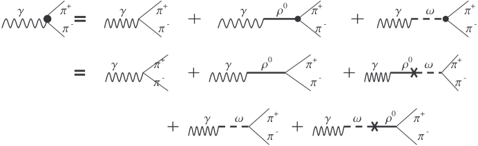
FIG. 2.: The Electromagnetic(EM) pion form factor. Indications of the lines for the propagators are same as Fig.1. The black dots are form factors.

Now, we study the anomalous-like $\rho^{0}\rightarrow\pi^{0}\gamma$ and $\omega\rightarrow\pi^{0}\gamma$ decays in terms of the expt-MP approach. Namely, taking $X=\pi^{0}\gamma$ in eq.Β (52), we have

$\displaystyle D^{P}_{\rho\rho}f^{F}_{\rho^{0}\pi^{0}\gamma}$ $\displaystyle=$ $\displaystyle D^{P}_{\rho\rho}f_{\rho^{0}\pi^{0}\gamma}^{P}+D^{P}_{\rho\omega}f_{\omega\pi^{0}\gamma}^{P},$ (58)
$\displaystyle D^{P}_{\omega\omega}f^{F}_{\omega\pi^{0}\gamma}$ $\displaystyle=$ $\displaystyle D^{P}_{\omega\omega}f_{\omega\pi^{0}\gamma}^{P}+D^{P}_{\omega\rho}f_{\rho^{0}\pi^{0}\gamma}^{P},$ (59)

and hence

$\displaystyle f^{F}_{\rho^{0}\pi^{0}\gamma}$ $\displaystyle=$ $\displaystyle f_{\rho^{0}\pi^{0}\gamma}^{(0)}-\eta f_{\omega\pi^{0}\gamma}^{(0)}+{T\over m_{\rho}^{2}-m_{\omega}^{2}+im_{\omega}\Gamma_{\omega}}f_{\omega\pi^{0}\gamma}^{(0)},$ (60)
$\displaystyle f^{F}_{\omega\pi^{0}\gamma}$ $\displaystyle=$ $\displaystyle f_{\omega\pi^{0}\gamma}^{(0)}+\eta f_{\rho^{0}\pi^{0}\gamma}^{(0)}+{T\over m_{\omega}^{2}-m_{\rho}^{2}+im_{\rho}\Gamma_{\rho}}f_{\rho\pi^{0}\gamma}^{(0)},$ (61)

where eqs.(Β 38) and (Β 43) have been used. Considering $|\eta|\simeq 0.006<<1$ and T≃Πρ​ωsimilar-to-or-equals𝑇subscriptΞ πœŒπœ”T\simeq\Pi_{\rho\omega}, we finally obtain the desired results in the expt-MP formalism as follows

$\displaystyle f_{\rho^{0}\pi^{0}\gamma}|_{\rm expt-MP}$ $\displaystyle\equiv$ fρ0​π0​γF≃fρ0​π0​γ(0)+Πρ​ωmρ2βˆ’mΟ‰2+i​mω​Γω​fω​π0​γ(0),similar-to-or-equalssubscriptsuperscript𝑓𝐹superscript𝜌0superscriptπœ‹0𝛾superscriptsubscript𝑓superscript𝜌0superscriptπœ‹0𝛾0subscriptΞ πœŒπœ”superscriptsubscriptπ‘šπœŒ2superscriptsubscriptπ‘šπœ”2𝑖subscriptπ‘šπœ”subscriptΞ“πœ”superscriptsubscriptπ‘“πœ”superscriptπœ‹0𝛾0\displaystyle f^{F}_{\rho^{0}\pi^{0}\gamma}\simeq f_{\rho^{0}\pi^{0}\gamma}^{(0)}+{\Pi_{\rho\omega}\over m_{\rho}^{2}-m_{\omega}^{2}+im_{\omega}\Gamma_{\omega}}f_{\omega\pi^{0}\gamma}^{(0)}, (62)
$\displaystyle f_{\omega\pi^{0}\gamma}|_{\rm expt-MP}$ $\displaystyle\equiv$ fω​π0​γF≃fω​π0​γ(0)+Πρ​ωmΟ‰2βˆ’mρ2+i​mρ​Γρ​fρ0​π0​γ(0).similar-to-or-equalssubscriptsuperscriptπ‘“πΉπœ”superscriptπœ‹0𝛾superscriptsubscriptπ‘“πœ”superscriptπœ‹0𝛾0subscriptΞ πœŒπœ”superscriptsubscriptπ‘šπœ”2superscriptsubscriptπ‘šπœŒ2𝑖subscriptπ‘šπœŒsubscriptΞ“πœŒsuperscriptsubscript𝑓superscript𝜌0superscriptπœ‹0𝛾0\displaystyle f^{F}_{\omega\pi^{0}\gamma}\simeq f_{\omega\pi^{0}\gamma}^{(0)}+{\Pi_{\rho\omega}\over m_{\omega}^{2}-m_{\rho}^{2}+im_{\rho}\Gamma_{\rho}}f_{\rho^{0}\pi^{0}\gamma}^{(0)}. (63)

Noting $f_{\omega\pi^{0}\gamma}^{(0)}=3f_{\rho^{0}\pi^{0}\gamma}^{(0)}$, above equations are same as eq.(1). Consequently, this result indicates that the charge-asymmetry enhancement effect to $\rho^{0}\rightarrow\pi\gamma$ revealed in ref.[4] by using the effective Lagrangian theory has been confirmed in expt-PM approach.

To conclude, the Mixed Propagator (MP) approach to $\rho-\omega$ mixing is investigated in this letter. It is found that under the pole-approximation assumption the results of MP approach is not compatible both with the effective Lagrangian theory and with the experiment measurement criterion. This fact indicates the pole approximation for determining the physical basis of $\rho$ and $\omega$ is inadequate and ad hoc. To cure these diseases, we propose a new MP approach in which the physical states of $\rho$ and $\omega$ are determined by the requirement of experimental measurement to meson resonance. In terms of this new MP approach, the EM pion form factor $F_{\pi}$ and form factors of $\rho^{0}\rightarrow\pi^{0}\gamma$ and of $\omega\rightarrow\pi^{0}\gamma$ are derived. The results of $F_{\pi}$ are in good agreement with data. The form factor of $\rho^{0}\rightarrow\pi^{0}\gamma$ exhibits a hidden charge-asymmetry enhancement effect which agree with the prediction of the effective Lagrangian theory, i.e., the conclusion of ref.[4] has been confirmed.

We are pleased to acknowledge K.F.Liu for helpful discussion.

REFERENCES

  • [1] S.Glashow, Phys.Rev.Lett., 7, 469 (1961).
  • [2] H.B.O’Connell, B.C.Pearce, A.W.Thomas and A.G.Williams, Prog.Nucl.Part.Phys., 39, 201 (1997).
  • [3] F.M.Renard, Springer Tracts in Modern Phys., 63, 98-120, Springer Verlag (1972).
  • [4] X.J.Wang, J.H.Jiang and M.L.Yan,Isospin Symmetry Breaking in $\rho\rightarrow\pi\gamma$, hep-ph/0101166.
  • [5] M.Benayoun, S.I.Eidelman and V.N.Ivanchenko, Z.Phys., C72, 221 (1996).
  • [6] X.J.Wang and M.L.Yan, hep-ph/0010215; T.L.Zhuang, X.J.Wang and M.L.Yan, Phys. Rev., D62, 053007 (2000); D.N.Gao and M.L.Yan, Euro Phys Jour., A3, 293(1998) ; B.A.Li, Phys Rev., D52, 5156(1995); E.Jenkins, A.V. Manohar and M.B. Wise, Phys. Rev. Lett. 75, 2272(1995) ; A.K. Leibovich, A.V. Manohar and M.B. Wise, Phys. Lett. B358, 347(1995) ; J. Bijnens, P.Gosdzinsky and P. Talavera, Phys. Lett. B429, 111(1998) ; J.Bijinens, P. Gosdzinsky and P.Talavera, JHEP 9801, 014(1998) ; T.Hatsuda and T.Kunihiro, Phys. Rep. 247, 221(1994) ; M.Bando,T.Kugo and K.Yamawaki, Nucl. Phys. B259, 493(1985) , Prog. Theor. Phys. 79, 1140(1988) , Phys. Rep. 164, 217(1988) ; N.Kaiser and U.G.Meissner, Nucl. Phys., A519, 671(1990) . G.Eicker, J.Gasser, A.Pich and E.de Rafel, Nucl. Phys., B321, 311(1989) ; G.Eicker, H.Leutwyler, J.Gasser, A.Pich and E.de Rafel, Phys. Lett., B233, 425(1989) ; M.Brise, Z.Phys., 355, 231(1996) ; J.Bijinens, P.Gosdzinsky and P.Talavera, Nucl. Phys., B501, 495(1997) ; J.Bijnens, Phys. Rep. 265, 369(1996).
  • [7] X.J. Wang and M.L. Yan, Phys. Rev. D 62, 094013 (2000).
  • [8] e.g., see: M.E.Peskin and D.V.Schroeder, An Introduction to Quantum Field Theory, Addison-Wesley Pub. Com., (1995), pp237.
  • [9] S.Gardner and H.B.O’Connell, Phys Rev., D57 2716 (1998).
  • [10] H.B.O’Connell,B.C.Pearce,A.W.Thinas,A.G.Williams,A.G.: Phys. Lett. B336,1 (1994) .
  • [11] M.Benayoun, S.Eidelman, K.Maltman, H.B.O’Connell, B.Shwartz and A.G.Williams, Europ. Phys. Jour., C2, 269 (1998); K.Maltman, H.B.O’Connell and A.G.Williams, Phys. Lett., B376, 19 (1996); S.Gardner and H.B.O’Connell, Phys. Rev., D57, 2716 (1998).