$N$-Point Vertex Functions, Ward-Takahashi Identities and
Dyson-Schwinger Equations in Thermal QCD/QED
in the Real Time Hard-Thermal-Loop Approximation

Abstract

In this paper we calculated the $n$-point hard-thermal-loop (HTL) vertex functions in QCD/QED for $n$= 2, 3 and 4 in the physical representation in the real time formalism (RTF). The result showed that the $n$-point HTL vertex functions can be classified into two groups, a) those with odd numbers of external retarded indices, and b) the others with even numbers of external retarded indices. The $n$-point HTL vertex functions with one retarded index, which obviously belong to the first group a), are nothing but the HTL vertex functions that appear in the imaginary time formalism (ITF), and vise versa. All the HTL vertex functions belonging to the first group a) are of $O(g^{2}T^{2})$ , and satisfy among them the simple QED-type Ward-Takahashi identities, as in the ITF. Those vertex functions belonging to the second group b) never appear in the ITF, namely their existence is characteristic of the RTF, and their HTL’s have the high temperature behavior of $O(g^{2}T^{3})$, one-power of $T$ higher than usual. Despite this difference we could verify that those HTL vertex functions belonging to the second group b) also satisfy among themselves the QED-type Ward-Takahashi identities, thus guaranteeing the gauge invariance of the HTL’s in the real time thermal QCD/QED.

I Introduction and summary

The hard-thermal-loop (HTL) resummed effective perturbation theory of Braaten and Pisarski 1 ; 2 has given us in finite temperature (or thermal) field theory 3 ; 4 a procedure correctly estimating/extracting the dominant temperature effect due to the semi-classical thermal fluctuation. HTL’s are originally determined in the imaginary time formulation of thermal field theory 1 ; 2 by computing the one-loop diagrams. For calculating the Feynman diagrams in thermal field theory there are essentially two different formulations, namely the imaginary time formalism (ITF) and the real time formalisn(RTF) 3 ; 4 ; 5 . The ITF is restricted to calculating the static quantities in equilibrium, while the RTF is indispensable for analysing the dynamical quantities and for investigating the out-of-(or non)-equilibrium system thus for studying the physics of quark-gluon plasma.

The relation between quantities calculated in the ITF and in the RTF has been studied so far 6 ; the $n$-point function in the ITF corresponds to a specific sum of the $n$-point functions in the RTF, the same is true for the $n$-point HTL functions. In the ITF all the $n$-point HTL functions have been obtained, and are shown to be ultraviolet finite, gauge invariant and to satisfy simple Ward-Takahashi identities 1 ; 2 . Also in the RTF the $n$-point HTL functions ($n$=2, 3, 4) and their spectral functions have been partly determined 7 ; 8 , but the explicit expressions of the full $n$-point HTL functions have not been consistently given yet f1 . Even with such a limited knowledge on the $n$-point HTL functions in the RTF, analyses of the 3-point functions have shown 8 ; 9 that there exist the HTL functions being proportional to $g^{2}T^{3}$ ($g$: the coupling constant, and $T$: the temperature of the environment), never existing in the ITF where all the $n$-point HTL functions being proportional to $g^{2}T^{2}$. Here it is worth noting that in the RTF the Ward-Takahashi identities have been confirmed to hold only among the ITF counterparts, namely among the special linear combinations of $n$-point HTL functions corresponding to those in the ITF, having not been seen anything among those HTL functions not existing in the ITF.

Recently beginning of the relativistic heavy ion collision experiments at BNL-RHIC has attracted an increasing interest in studying the physics in thermal QCD. Progress of the physics of quark-gluon plasma and the development of the calculational framework towards the system in non-(or out-of-)equilibrium have urged us to determine explicitly all the HTL’s in the RTF with the relations such as the Ward-Takahashi identities they might have satisfied.

In this paper we determine explicitly in the RTF, especially in the ”physical representation” in the closed-time-path (CTP), or the Keldysh formalism 4 ; 5 , the HTL contributions to the $n$-point vertex functions in thermal QCD/QED with $n$=2, 3, 4 which are in urgent demand. Also studied are the structure of the Ward-Takahashi identities that might be satisfied among them. As an application we write down the Dyson-Schwinger equations in the HTL approximation for the fermion mass function. Results can be summarized briefly as follows f2 ;

i) In the RTF there are two types of $n$-point vertex functions having the HTL contributions; one is the vertex function with $n$ external gauge bosons ($n$g vertex function) and the other with a pair of external fermions and ($n$-2) external gauge bosons (2f-($n$-2)g vertex function). There are no other $n$-point HTL functions, thus there are no $n$-point HTL functions with external ghost lines. This situation is completely the same as in the ITF 1 .

ii) All the $n$-point HTL vertex functions with one retarded index in the physical representation in the CTP formalism take exactly the same expressions (thus are proportional to $g^{2}T^{2}$) as those analytically continued from the $n$-point HTL vertex functions determined in the ITF through simple but corresponding continuation paths. They satisfy the same Ward-Takahashi identities as those in the ITF 1 ; 2 . The $n$-point vertex functions with one retarded index ($V_{RAA},V_{ARA},V_{RAAA},V_{ARAA}$, etc) are nothing but the functions exactly corresponding to the $n$-point vertex functions that can be calculated in the ITF, and are given by the specific sum (for details, see section II) of those in the ”single time representation” in the CTP formalism, where a given $n$-point Feynman diagram contains a Keldish index at each end (external vertex) taking values {1,2}, corresponding to the two branches of the closed-time-path contour.

iii) The $n$-point ($n$=2, 3, 4) vertex functions with two retarded indices ($V_{RRA},V_{RRAA}$, etc) are characteristic of the RTF, never appearing in the ITF. The corresponding $n$-point HTL vertex functions must be classified into two groups: the $n$g vertex functions and the 2f-($n$-2)g vertex functions. Other types of $n$-point vertex functions in general never have the HTL contributions as mentioned in i) above. It is quite remarkable that in QCD the $n$g vertex functions with two retarded indices are proportional to $g^{2}T^{3}$ in contrast to the $O(g^{2}T^{2})$ behavior of the usual HTL vertex functions, thus are expected to play important roles in studying the temperature effects. Nevertheless we can verify that they satisfy the QED-type Ward-Takahashi identities between the corresponding $n$g- and ($n$-1)g HTL vertex functions, still guaranteeing the gauge invariance of the HTL approximation. Thus we can prove, through the explicit calculations of the $n$-point HTL vertex functions, the gauge invariance of the real time thermal QCD/QED in the HTL approximation. It is also worth noting that the HTL contributions to the 2f-($n$-2)g vertex functions with two retarded indices totally vanish f3 , thus in QED there are no additional HTL functions other than those appeared in the ITF.

iv) In performing the calculation of the Feynman diagrams in the RTF we should be very careful for the treatment of the singular functions (the Dirac-$\delta$ function and the principal part) appearing in the free propagators. We must use the properly regularized forms during the calculation and should take the limit $\varepsilon\ \rightarrow 0$ at the end of all calculations, as noted by Landsman and van Wheert 4 .

v) We explicitly write down the HTL resummed Dyson-Schwinger equation for the physical fermion mass function, namely the retarded fermion self-energy function, in thermal QCD/QED, which can be used to investigate the nature of the chiral phase transition at finite temperature. Some comment on the double counting problem is also given.

This paper is organized as follows. In the next section II we give a brief review of the ”physical representation” in the Keldysh or the CPT formalism. In section III the $n$-point HTL vertex functions ($n$=2, 3, 4) are explicitly determined in the physical representation. The necessity of the use of regularized form of the singular functions is demonstrated. The HTL Ward-Takahashi identities between the four- and three-point functions together with the three- and two-point functions are explicitly verified. As an application the Dyson-Schwinger equations in the HTL approximation for the physical fermion mass function $\Sigma_{R}$ is derived in section V. Conclusions and some discussion are given in the last section VI.

II Real Time Closed-Time-Path or the Keldysh Formalism

We use the closed-time-path (CTP) or the Keldysh formalism 4 ; 5 of the RTF throughout this paper. In this formalism there are two familiar representations, namely by following the terminology of Ref.4 , the ”single time” representation and the ”physical”, or the ”retarded-advanced” representation. In the single time representation the single-particle propagator for free bosons has the 2 $\times$ 2 matrix form

$$\hat{D}(K)=\left(\begin{array}[]{ll}D_{11}(K)&D_{12}(K)\\ D_{21}(K)&D_{22}(K)\\ \end{array}\right),$$ (II.1)

$D_{ij}\ (i,j=1,2)$ are given in momentum space by

$$D_{11}(K) = \frac{1+n_{B}(k_{0})}{K^{2}-m^{2}+i\varepsilon}-\frac{n_{B}(k_{0})}{K^{2}-m^{2}-i\varepsilon}\ ,$$ (II.2a)

$$D_{12}(K) = [\theta(-k_{0})+n_{B}(k_{0})]\left(\frac{1}{K^{2}-m^{2}+i\varepsilon}-\frac{1}{K^{2}-m^{2}-i\varepsilon}\right)\ ,$$ (II.2b)

$$D_{21}(K) = [\theta(k_{0})+n_{B}(k_{0})]\left(\frac{1}{K^{2}-m^{2}+i\varepsilon}-\frac{1}{K^{2}-m^{2}-i\varepsilon}\right)\ ,$$ (II.2c)

$$D_{22}(K) = \frac{n_{B}(k_{0})}{K^{2}-m^{2}+i\varepsilon}-\frac{1+n_{B}(k_{0})}{K^{2}-m^{2}-i\varepsilon}\ ,$$ (II.2d)

where $K=(k_{0},\mbox{\boldmath{$k$}})$, $\theta$ denotes the step function, and the equilibrium distribution function is given by $n_{B}(k_{0})=1/[\exp(|k_{0}|/T)-1]$. For fermions the bare propagator can be also written as the 2 $\times$ 2 matrix form

$$\hat{S}(K)=\left(\begin{array}[]{ll}S_{11}(K)&S_{12}(K)\\ S_{21}(K)&S_{22}(K)\\ \end{array}\right),$$ (II.3)

and

$$S_{ij} = (\not{\!K}-m)\overline{D}_{ij}(K)\ ,$$ (II.4a)

$$\overline{D}_{ij} = D_{ij}\{n_{B}(k_{0})\rightarrow-n_{F}(k_{0})\}\ ,\ (i,j=1,2),$$ (II.4b)

where the Fermi-Dirac distribution is given by $n_{F}(k_{0})=1/[\exp(|k_{0}|/T)+1]$. Components of these propagators are not independent of each other. There is an algebraic identity

$$G_{11}+G_{22}=G_{12}+G_{21},$$ (II.5)

where $G$ stands for $D$ or $S$, respectively.

By an orthogonal transformation

$$\hat{G} = Q^{-1}\tilde{G}Q,\ \tilde{G}=Q\hat{G}Q^{-1};\ G=D\ \mbox{or}\ S\ ,$$ (II.6)

$$Q = \frac{1}{\sqrt{2}}(1-\sigma_{2})\ ,$$ (II.7)

we arrive at the propagator in the physical, or the retarded-advanced representation,

$$\tilde{D}(K)=\left(\begin{array}[]{ll}D_{AA}(K)&D_{AR}(K)\\ D_{RA}(K)&D_{RR}(K)\\ \end{array}\right),$$ (II.8)

and $D_{\alpha\beta}\ (\alpha,\ \beta=A,R)$ are

$$D_{AA}(K) = 0,$$ (II.9a)

$$D_{AR}(K)\ (\ \equiv D_{A}(K)) = \frac{1}{K^{2}-m^{2}-i\mbox{sgn}(k_{0})\varepsilon}\ ,$$ (II.9b)

$$D_{RA}(K)\ (\ \equiv D_{R}(K)) = \frac{1}{K^{2}-m^{2}+i\mbox{sgn}(k_{0})\varepsilon}\ ,$$ (II.9c)

$$D_{RR}(K)\ (\ \equiv D_{C}(K)) = (1+2n_{B}(k_{0}))\mbox{sgn}(k_{0})[D_{RA}(K)-D_{AR}(K)]\ ,$$ (II.9d)

for bosons and

$$\tilde{S}(K)=\left(\begin{array}[]{ll}S_{AA}(K)&S_{AR}(K)\\ S_{RA}(K)&S_{RR}(K)\\ \end{array}\right),$$ (II.10)

$$S_{AA}(K) = 0,$$ (II.11a)

$$S_{AR}(K)\ (\ \equiv S_{A}(K)) = (\not{\!K}-m)\frac{1}{K^{2}-m^{2}+i\mbox{sgn}(k_{0})\varepsilon}\ ,$$ (II.11b)

$$S_{RA}(K)\ (\ \equiv S_{R}(K)) = (\not{\!K}-m)\frac{1}{K^{2}-m^{2}-i\mbox{sgn}(k_{0})\varepsilon}\ ,$$ (II.11c)

$$S_{RR}(K)\ (\ \equiv S_{C}(K)) = (1-2n_{F}(k_{0}))\mbox{sgn}(k_{0})[S_{RA}(K)-S_{AR}(K)]\ ,$$ (II.11d)

for fermions, where the last equations in Eqs. (II.9) and (II.11) are consequences of the fluctuation-dissipation theorem.

Propagator (connected 2-point Green function) $G$ and the 1-particle irreducible 2-point vertex function $\Sigma$ satisfies the Dyson equation ($G=D$ or $S$, and correspondingly $\Sigma$ denotes the bosonic or fermionic 2-point vertex, i.e., self-energy function)

$$\int\hat{\Sigma}\sigma_{3}\hat{G} = \sigma_{3},\ \ \ \ \int\hat{G}\sigma_{3}\hat{\Sigma}=\sigma_{3},$$ (II.12a)

$$\int\tilde{\Sigma}\sigma_{1}\tilde{G} = \sigma_{1},\ \ \ \ \int\tilde{G}\sigma_{1}\tilde{\Sigma}=\sigma_{1}.$$ (II.12b)

In the above, the relations (II.1), (II.3), (II.5)-(II.8), (II.10) and (II.12) also hold for full propagators and full 2-point vertex functions.

It is also worth noticing here that in the above equations for the free propagators, Eqs. (II.1)-(II.4) and (II.8)-(II.11), we do not use the expressions that contain explicitly the singular functions themselves, but rather use the functions with the regularization parameter $\varepsilon$, e.g.,

$$\frac{1}{[K^{2}-m^{2}+i\varepsilon]}=\mbox{PP}\frac{1}{[K^{2}-m^{2}]}-i\pi\delta(K^{2}-m^{2}),$$ (II.13)

where

$$\mbox{PP}\frac{1}{x} \equiv \frac{x}{x^{2}+{\varepsilon}^{2}},$$ (II.14a)

$$\pi\delta(x) \equiv \frac{\varepsilon}{x^{2}+{\varepsilon}^{2}}.$$ (II.14b)

Keeping $\varepsilon$ finite (i.e., $\varepsilon\neq 0$) till the end of all calculations then taking the limit $\varepsilon\rightarrow 0$ at the end is extremely important as we shall explicitly see in the next section.

III The $n$-point ($n$=2, 3, 4) vertex functions in QCD/QED in the HTL approximation

In this section we calculate the HTL contributions to the one particle irreducible $n$-point vertex functions ($n$=2, 3, 4) in the physical or the retarded-advanced representation. One can construct in general the $n$-point vertex functions in the physical or the retarded-advanced representation from the components of the real-time $n$-point functions in the single time representation as in literature 4 ; 6 ; 7 ; 10 ; 11 , in which some care must be taken because the notation varies from literature to literature. Throughout this paper we use the notation as follows; a given one particle irreducible $n$-point Feynman diagram in the single time representation contains a Keldish index at each end (external vertex) taking values {1, 2}, corresponding to the two branches of the closed-time-path contour, while in the physical representation it contains a retarded-advanced index at each end taking values $\{R,\ A\}$, corresponding to the retarded or the advanced prescription. Our notation follows the one in Ref. 7 .

III.1 The $n$-point vertex functions ($n$=2, 3, 4) in the physical representation

For convenience we here present explicitly the 2-, 3-, and 4-point vertex functions in the physical representation constructed from the components in the single time representation. Generally speaking the $n$-point function has $2^{n}$ components. These components obey one constraint equation, which reduces the number of independent components to $2^{n}-1$. In the physical representation this is expressed by the fact that the $n$-point vertex function with $n$-external advanced indices automatically vanishes, Eqs. (III.1a), (III.3a) and (III.4a), below. In equilibrium, the Kubo-Martin-Schwinger conditions impose additional constraints, reducing the number of independent components to $2^{(n-1)}-1$. For details of the construction, see Refs.4 ; 7 . Since the transformation formula between the vertex functions in two representations do not take care of the external particle species (fermion or gauge boson), here we simply write $V_{\alpha\beta...\delta},\ \{\alpha,\beta,...,\delta=R,A\}$, or $V_{ij...l},\ \{i,j,...,l=1,2\}$ for vertex functions in the physical and the single time representations, respectively.

III.1.1 2-point vertex functions

$$V_{AA} = 0,$$ (III.1a)

$$V_{RA}\ (\ \equiv V_{R}) = V_{11}+V_{12},$$ (III.1b)

$$V_{AR}\ (\ \equiv V_{A}) = V_{11}+V_{21},$$ (III.1c)

$$V_{RR}\ (\ \equiv V_{C}) = V_{11}+V_{22}.$$ (III.1d)

Among them the following relations hold,

$$V_{AR}(K) = {V_{RA}}^{*}(K),$$ (III.2a)

$$V_{RR}(K) = \{1+\eta 2n(k_{0})\}\mbox{sgn}(k_{0})\{V_{RA}(K)-V_{AR}(K)\},$$ (III.2b)

where $\eta=+1(-1)$ for boson (fermion) and $n(k_{0})$ is the corresponding equilibrium distribution function.

III.1.2 3-point vertex functions

$$V_{AAA} = 0,$$ (III.3a)

$$V_{RAA} = V_{111}+V_{112}+V_{121}+V_{122},$$ (III.3b)

$$V_{ARA} = V_{111}+V_{112}+V_{211}+V_{212},$$ (III.3c)

$$V_{AAR} = V_{111}+V_{121}+V_{211}+V_{221},$$ (III.3d)

$$V_{RRA} = V_{111}+V_{112}+V_{221}+V_{222},$$ (III.3e)

$$V_{RAR} = V_{111}+V_{121}+V_{212}+V_{222},$$ (III.3f)

$$V_{ARR} = V_{111}+V_{211}+V_{122}+V_{222},$$ (III.3g)

$$V_{RRR} = V_{111}+V_{122}+V_{212}+V_{221}.$$ (III.3h)

The Kubo-Martin-Schwinger conditions impose additional 4 constraints, reducing the number of independent components to 3.

III.1.3 4-point vertex functions

$$V_{AAAA} = 0,$$ (III.4a)

$$V_{RAAA} = V_{1111}+V_{1112}+V_{1121}+V_{1211}+V_{1122}+V_{1212}+V_{1221}+V_{1222},$$ (III.4b)

$$V_{ARAA} = V_{1111}+V_{1112}+V_{1121}+V_{2111}+V_{1122}+V_{2112}+V_{2121}+V_{2122},$$ (III.4c)

$$V_{AARA} = V_{1111}+V_{1112}+V_{1211}+V_{2111}+V_{1212}+V_{2112}+V_{2211}+V_{2212},$$ (III.4d)

$$V_{AAAR} = V_{1111}+V_{1121}+V_{1211}+V_{2111}+V_{1221}+V_{2121}+V_{2211}+V_{2221},$$ (III.4e)

$$V_{RRAA} = V_{1111}+V_{1112}+V_{1121}+V_{1122}+V_{2211}+V_{2212}+V_{2221}+V_{2222},$$ (III.4f)

$$V_{RARA} = V_{1111}+V_{1112}+V_{1211}+V_{1212}+V_{2121}+V_{2122}+V_{2221}+V_{2222},$$ (III.4g)

$$V_{RAAR} = V_{1111}+V_{1121}+V_{1211}+V_{1221}+V_{2112}+V_{2122}+V_{2212}+V_{2222}.$$ (III.4h)

There are seven independent vertex functions, Eqs. (III.4a-h), in this case, and the other eight vertex functions can be obtained from them using the Kubo-Martin-Schwinger conditions.

III.2 The $n$-point vertex functions ($n$=2, 3, 4) in the HTL approximation

Now we calculate the $n$-point vertex functions ($n$=2, 3, 4) in the physical representation in the HTL approximation. In the following we consider the massless QCD/QED, namely the high temperature hot QCD/QED, where all the fermions and the gauge bosons are massless.

Because we are accustomed to the Feynman rules in the single time representation, we calculate explicitly the right-hand-side of Eqs. (III.1), (III.3) and (III.4). As we have stressed at the end of the last section we use Eqs. (II.13) and (II.14) for propagators, namely, we do not use the expressions that contain explicitly the singular functions themselves, but rather use the functions with the regularization parameter $\varepsilon$ and keep $\varepsilon$ finite (i.e., $\varepsilon\neq 0$) till the end of all calculations then take the limit $\varepsilon\ \rightarrow\ 0$ at the end.

III.2.1 2-point vertex functions, or the fermion self-energy and the gauge boson polarization tensor

The 2-point vertex function in QCD/QED is usually named as the self-energy part $\Sigma$ for fermion, while it is called as the (vacuum) polarization tensor $\Pi^{\mu\nu}$ for gauge boson (gluon/photon). Although the HTL results of $\Sigma$ and $\Pi^{\mu\nu}$ in the single time representation as well as in the ITF are already well-known 1 ; 12 ; 13 , for the sake of completeness we here present the results in the physical representation. In fact in calculating their HTL contributions in the physical representation, some care being worth mentioning must be taken, obtaining the result that could not be seen, at least in the explicit form, in the previous calculations 1 ; 12 .

The HTL contribution to the fermion self energy, $\delta\Sigma$, in the single time representation is obtained in QCD by calculating the diagram shown in Fig.1 (in QED $g^{2}C_{F}$ should read $e^{2}$);

$$-i\delta\Sigma_{ij}(P,Q)=2g^{2}C_{F}\int\frac{d^{4}K}{(2\pi)^{4}}\not{\!K}\overline{D}_{ij}(K+Q)D_{ji}(K),\ \ \ P+Q=0,$$ (III.5)

where $D_{ij}$ and $\overline{D}_{ij}$ are given in Eqs.(II.2) and (II.4). With the use of Eqs.(III.1) we get the HTL fermion self energy in the physical representation. There are nothing new in the obtained results in QCD, thus only reproducing the previous results;

$$\delta\Sigma_{RA}(P,Q) = -\frac{g^{2}C_{F}}{32\pi}T^{2}\int d\Omega\frac{\hat{\not{\!K}}}{Q\cdot\hat{K}+i\varepsilon},$$ (III.6a)

$$\delta\Sigma_{AR}(P,Q) = -\frac{g^{2}C_{F}}{32\pi}T^{2}\int d\Omega\frac{\hat{\not{\!K}}}{Q\cdot\hat{K}-i\varepsilon},$$ (III.6b)

$$\delta\Sigma_{RR}(P,Q) = 0,$$ (III.6c)

where $\hat{K}^{\mu}=(1,\hat{\mbox{\boldmath{$k$}}})$ with $\hat{\mbox{\boldmath{$k$}}}\ \equiv\ \mbox{\boldmath{$k$}}/k,\ k=\sqrt{{\mbox{\boldmath{$k$}}}^{2}}$, being the unit three vector along the direction of $k$.

As was expressed in Eqs.(III.1) we usually denote the $\{RA\}$-component as the $R$-, or the retarded component, and the $\{AR\}$-component as the $A$-, or the advanced component of the corresponding quantity. Namely $\Sigma_{RA}\equiv\Sigma_{R}$ is the fermion self-energy part of the inverse retarded fermion propagator, having a definite physical meaning, i.e., the physical fermion mass function.

As for the HTL contribution to the gauge boson polarization tensor, $\delta\Pi^{\mu\nu}$, the diagrams to be calculated in the single time representation are shown in Fig. 2 $(P+Q=0)$ ;

$$i\delta\Pi^{\mu\nu}_{ij}(P,Q)=\left\{\begin{array}[]{ll}-4e^{2}(-1)^{i+j-2}\int\frac{\displaystyle{d^{4}K}}{\displaystyle{(2\pi)^{4}}}\left[2K^{\mu}K^{\nu}-g^{\mu\nu}K^{2}\right]\overline{D}_{ij}(K)\overline{D}_{ji}(K+P),&\mbox{(QED)}\\ &\\ 2g^{2}(-1)^{i+j-2}\int\frac{\displaystyle{d^{4}K}}{\displaystyle{(2\pi)^{4}}}\left[2K^{\mu}K^{\nu}-g^{\mu\nu}K^{2}\right]&\\ \ \ \times\left\{N_{c}{D}_{ij}(K){D}_{ji}(K+P)-N_{f}\overline{D}_{ij}(K)\overline{D}_{ji}(K+P)\right\},&(QCD)\\ \end{array}\right.$$ (III.7)

from which we get the HTL gluon polarization tensor in QCD (for the photon polarization tensor in QED, $g^{2}(N_{c}+(1/2)N_{f})$ should be understood as $e^{2}$),

$$\delta\Pi^{\mu\nu}_{RA}(P,Q) = -\frac{g^{2}T^{2}}{12\pi}\left(N_{c}+\frac{1}{2}N_{f}\right)\int d\Omega\left({\hat{K}^{\mu}\hat{K}^{\nu}}\frac{q_{0}}{\hat{K}{\cdot}Q+i\varepsilon}-g^{\mu 0}g^{\nu 0}\right),$$ (III.8a)

$$\delta\Pi^{\mu\nu}_{AR}(P,Q) = -\frac{g^{2}T^{2}}{12\pi}\left(N_{c}+\frac{1}{2}N_{f}\right)\int d\Omega\left({\hat{K}^{\mu}\hat{K}^{\nu}}\frac{q_{0}}{\hat{K}{\cdot}Q-i\varepsilon}-g^{\mu 0}g^{\nu 0}\right),$$ (III.8b)

$$\delta\Pi^{\mu\nu}_{RR}(P,Q) = -\frac{g^{2}T^{3}}{6\pi}\left(N_{c}+\frac{1}{2}N_{f}\right)\int d\Omega\hat{K}^{\mu}\hat{K}^{\nu}\left(\frac{1}{\hat{K}{\cdot}Q+i\varepsilon}-\frac{1}{\hat{K}{\cdot}Q-i\varepsilon}\right).$$ (III.8c)

Same as the fermion self-energy function $\Pi^{\mu\nu}_{RA}(\Pi^{\mu\nu}_{AR})\equiv\Pi^{\mu\nu}_{R}(\Pi^{\mu\nu}_{A})$ is the gauge boson polarization tensor in the inverse retarded (advanced) gauge boson propagator, thus having a definite physical meaning.

It should be noted that the $\{RR\}$-component of the polarization tensor, $\delta\Pi^{\mu\nu}_{RR}$, is proportional to $g^{2}T^{3}$, compared to the ordinary retarded or advanced polarization tensor, $\delta\Pi^{\mu\nu}_{RA}$ or $\delta\Pi^{\mu\nu}_{AR}$, being proportional to $g^{2}T^{2}$. Also noted is that all the HTL contribution in the ITF are of the order $O(g^{2}T^{2})$, thus the above results show completely new vertex functions appear in the RTF.

III.2.2 3-point vertex functions

There are two types of 3-point vertex functions, the fermion-gauge-boson vertex function and the 3-gauge-boson vertex function. Needless to say in QED only the fermion-gauge-boson vertex function exists.

The fermion-gauge-boson vertex functions

We define the fermion-gauge-boson vertex function in the HTL approximation as in Fig.3, where

$$\ {}^{*}\Gamma^{\mu}=\gamma^{\mu}+\delta\Gamma^{\mu},$$ (III.9a)

with $$\gamma^{\mu}$$ representing the tree vertex

$$\gamma^{\mu}_{ijk} = (-)^{(i-1)}\gamma^{\mu},\ \ \ i=j=k,$$ (III.9b)

$$= 0\ ,\ \ \ \ \ \ \ \ \ \ \ \ \ \ \ \ \mbox{otherwise},$$

and the HTL contribution to the fermion-gauge-boson vertex function, $\delta\Gamma^{\mu}$, is obtained by calculating the one-loop diagrams shown in Fig.4;

$$\delta\Gamma^{\mu}_{ijk}(P,Q,R)=\left\{\begin{array}[]{ll}4ie^{2}\int\frac{\displaystyle{d^{4}K}}{\displaystyle{(2\pi)^{4}}}K^{\mu}\not{\!K}\tilde{V}_{ijk}\ ,&\mbox{(QED)}\\ 4ig^{2}C_{F}\int\frac{\displaystyle{d^{4}K}}{\displaystyle{(2\pi)^{4}}}K^{\mu}\not{\!K}\tilde{V}_{ijk}-2ig^{2}N_{c}\int\frac{\displaystyle{d^{4}K}}{\displaystyle{(2\pi)^{4}}}K^{\mu}\not{\!K}\left(\tilde{V}_{ijk}+V_{ijk}\right)\ ,&\mbox{(QCD)}\\ \end{array}\right.$$ (III.10c)

where,

$$V_{ijk}\ \equiv\ (-1)^{i+j+k-3}\overline{D}_{ij}(K)D_{jk}(K-Q)D_{ki}(K+P)\ ,$$ (III.10d)

$$\tilde{V}_{ijk}\ \equiv\ (-1)^{i+j+k-3}{D}_{ij}(K)\overline{D}_{jk}(K-Q)\overline{D}_{ki}(K+P)\ .$$ (III.10e)

The results in QCD in the physical representation are given as follows (in QED $g^{2}C_{F}$ should be understood as $e^{2}$);

$$\delta\Gamma^{\mu}_{RAA}(P,Q,R) = -\frac{g^{2}T^{2}}{32\pi}C_{F}\int d\Omega\frac{\hat{K}^{\mu}\not{\!\hat{K}}}{(\hat{K}{\cdot}P-i\varepsilon)(\hat{K}{\cdot}Q+i\varepsilon)}\ ,$$ (III.11a)

$$\delta\Gamma^{\mu}_{ARA}(P,Q,R) = -\frac{g^{2}T^{2}}{32\pi}C_{F}\int d\Omega\frac{\hat{K}^{\mu}\not{\!\hat{K}}}{(\hat{K}{\cdot}P+i\varepsilon)(\hat{K}{\cdot}Q-i\varepsilon)}\ ,$$ (III.11b)

$$\delta\Gamma^{\mu}_{AAR}(P,Q,R) = -\frac{g^{2}T^{2}}{32\pi}C_{F}\int d\Omega\frac{\hat{K}^{\mu}\not{\!\hat{K}}}{(\hat{K}{\cdot}P+i\varepsilon)(\hat{K}{\cdot}Q+i\varepsilon)}\ ,$$ (III.11c)

$$\delta\Gamma^{\mu}_{RRR}(P,Q,R) = -\frac{g^{2}T^{2}}{32\pi}C_{F}\int d\Omega\frac{\hat{K}^{\mu}\not{\!\hat{K}}}{(\hat{K}{\cdot}P-i\varepsilon)(\hat{K}{\cdot}Q-i\varepsilon)}\ ,$$ (III.11d)

$$\delta\Gamma^{\mu}_{RRA}(P,Q,R) = \delta\Gamma^{\mu}_{RAR}(P,Q,R)=\delta\Gamma^{\mu}_{ARR}(P,Q,R)=\delta\Gamma^{\mu}_{AAA}(P,Q,R)=0\ .$$ (III.11e)

We can see that all the HTL terms of the fermion-gauge-boson vertex function, $\delta\Gamma^{\mu}$, are proportional to $g^{2}T^{2}$.

In obtaining above results it is important to use the regularized expressions for free propagators with the finite regularization parameter $\varepsilon\ (\ \neq 0)$, Eqs. (II.1)-(II.4) and (II.13)-(II.14), not using the expressions in terms of the explicit singular functions from the beginning. To see this point more clearly let us calculate the above HTL vertex function $\delta\Gamma^{\mu}_{RAA}$, Eq.(III.11a), explicitly in QED. In each calculation of (III.11a-d) we must evaluate four diagrams in the single time representation, Eqs.(III.3), thus face the calculation, e.g., of $\delta\Gamma^{\mu}_{111}(P,Q,R)$,

$$\delta\Gamma^{\mu}_{111}(P,Q,R)=4ie^{2}\int\frac{d^{4}K}{(2\pi)^{4}}{D}_{11}(K)\overline{D}_{11}(K-Q)\overline{D}_{11}(K+P).$$ (III.12)

The loop-momentum integration over $K^{\mu}$ should be performed by keeping every $\varepsilon_{i}$ finite (i.e., $\varepsilon_{i}\neq 0$). Then the singularities of the integrand as a function of $k_{0}$ are only poles in the complex $k_{0}$-plane thus the integration over $k_{0}$ can be carried out through the residue analysis. By neglecting the $O(e^{2}T)$ contributions we get after some manipulations (here we set $\varepsilon_{1}=\varepsilon_{2}=\varepsilon_{3}=\varepsilon)$

$$\delta\Gamma^{\mu}_{111}(P,Q,R)=-\frac{e^{2}}{(2\pi)^{3}}\int dkkn(k)d\Omega K_{+}^{\mu}{\not{\!K}_{+}}\frac{K_{+}P}{(K_{+}P)^{2}+(\varepsilon)^{2}}\frac{K_{+}Q}{(K_{+}Q)^{2}+(\varepsilon)^{2}},$$ (III.13)

where $n(k)=n_{B}(k)+n_{F}(k)$ and $K_{+}^{\mu}=k(1,\hat{\mbox{\boldmath$k$}})=k\hat{K}^{\mu}$ with $\hat{\mbox{\boldmath{$k$}}}=\mbox{\boldmath{$k$}}/k$. Similar calculation gives

$$\delta\Gamma^{\mu}_{112}(P,Q,R) = -\frac{e^{2}}{(2\pi)^{3}}\int dkkn(k)d\Omega K_{+}^{\mu}{\not{\!K}_{+}}\frac{\varepsilon}{(K_{+}P)^{2}+(\varepsilon)^{2}}\frac{\varepsilon}{(K_{+}Q)^{2}+(\varepsilon)^{2}}\ ,$$ (III.14a)

$$\delta\Gamma^{\mu}_{121}(P,Q,R) = -i\frac{e^{2}}{(2\pi)^{3}}\int dkkn(k)d\Omega K_{+}^{\mu}{\not{\!K}_{+}}\frac{K_{+}P}{(K_{+}P)^{2}+(\varepsilon)^{2}}\frac{\varepsilon}{(K_{+}Q)^{2}+(\varepsilon)^{2}}\ ,$$ (III.14b)

$$\delta\Gamma^{\mu}_{122}(P,Q,R) = i\frac{e^{2}}{(2\pi)^{3}}\int dkkn(k)d\Omega K_{+}^{\mu}{\not{\!K}_{+}}\frac{\varepsilon}{(K_{+}P)^{2}+(\varepsilon)^{2}}\frac{K_{+}Q}{(K_{+}Q)^{2}+(\varepsilon)^{2}}\ .$$ (III.14c)

Adding Eqs.(III.13), (III.14a-c) we get Eq.(III.11a).

If we take naively the limit $\varepsilon_{i}\rightarrow 0$ before the loop-momentum integration over $K^{\mu}$, and use in Eq.(III.12) the free propagators explicitly containing the singular Dirac-$\delta$ function and the principal part, then the naive manipulation gives, instead of Eq.(III.13),

$$\delta\Gamma^{\mu}_{111}(P,Q,R)=-\frac{e^{2}}{(2\pi)^{3}}\int dkkn(k)d\Omega K_{+}^{\mu}{\not{\!K}_{+}}\left[\mbox{PP}\frac{1}{K_{+}P}\mbox{PP}\frac{1}{K_{+}Q}+\frac{\pi^{2}}{3}\delta(K_{+}P)\delta(K_{+}Q)\right].$$

Other three vertex functions coincide with the $\varepsilon_{i}\rightarrow 0$ limit of Eqs.(III.14a-c) and we can not get Eq.(III.11a). Additional term in Eq.(III.13’) being proportional to the product of Dirac-$\delta$ functions may have its origin from the integral whose integrand being the product of two principal parts

$$\int dy\int dx\mbox{PP}[\frac{1}{x-a(y)}]\mbox{PP}[\frac{1}{x-b(y)}].$$ (III.15)

If, at some $y=y_{0}$ inside the integration range over $y$, $a(y)=b(y)$ happens then we face the integration over $x$ of the square of principal part, which can not be well-defined. This is exactly what happens in the above calculation of Eq. (III.12) with the free propagators explicitly containing the singular Dirac-$\delta$ function and the principal part. Without concrete and consistent prescriptions how to treat the product of singular functions we can not get a definite result, and the $\varepsilon$-regularization method gives such a prescription. As we have already noted throughout this paper we use the $\varepsilon$-regularized singular functions.

Three gauge-boson (three gluon) vertex functions

We define the three gluon vertex function in the HTL approximation as in Fig.5, where

$$\ {}^{*}\Gamma^{\mu\nu\rho}=V^{\mu\nu\rho}+\delta\Gamma^{\mu\nu\rho},$$ (III.16)

with $V^{\mu\nu\rho}$ representing the tree vertex, which does not exist when the number of external retarded indices are zero or two. The HTL contribution to the three gluon vertex function, $\delta\Gamma^{\mu\nu\rho}$, is obtained by calculating the one-loop diagrams shown in Fig.6;

$$\delta\Gamma^{\mu\nu\rho}_{ijk}(P,Q,R) = -\frac{ig^{2}}{2\pi^{4}}(-1)^{i+k+j-3}\int d^{4}KK^{\mu}K^{\nu}K^{\rho}$$ (III.17)

$$\times \left[N_{c}D_{ij}(K)D_{jk}(K-Q)D_{ki}(K+P)-N_{f}\overline{D}_{ij}(K)\overline{D}_{jk}(K-Q)\overline{D}_{ki}(K+P)\right].$$

By using Eqs.(III.3) we get the HTL results in the physical representation;

$$\delta\Gamma^{\mu\nu\rho}_{RAA}(P,Q,R) = -\frac{g^{2}T^{2}}{12\pi}\left(N_{c}+\frac{1}{2}N_{f}\right)\int d\Omega\hat{K}^{\mu}\hat{K}^{\nu}\hat{K}^{\rho}\left[\frac{p_{0}}{(\hat{K}{\cdot}P-i\varepsilon)(\hat{K}{\cdot}R+i\varepsilon)}-\frac{q_{0}}{(\hat{K}{\cdot}Q+i\varepsilon)(\hat{K}{\cdot}R+i\varepsilon)}\right],$$

$$\delta\Gamma^{\mu\nu\rho}_{ARA}(P,Q,R) = -\frac{g^{2}T^{2}}{12\pi}\left(N_{c}+\frac{1}{2}N_{f}\right)\int d\Omega\hat{K}^{\mu}\hat{K}^{\nu}\hat{K}^{\rho}\left[\frac{p_{0}}{(\hat{K}{\cdot}P+i\varepsilon)(\hat{K}{\cdot}R+i\varepsilon)}-\frac{q_{0}}{(\hat{K}{\cdot}Q-i\varepsilon)(\hat{K}{\cdot}R+i\varepsilon)}\right],$$

$$\delta\Gamma^{\mu\nu\rho}_{AAR}(P,Q,R) = -\frac{g^{2}T^{2}}{12\pi}\left(N_{c}+\frac{1}{2}N_{f}\right)\int d\Omega\hat{K}^{\mu}\hat{K}^{\nu}\hat{K}^{\rho}\left[\frac{p_{0}}{(\hat{K}{\cdot}P+i\varepsilon)(\hat{K}{\cdot}R-i\varepsilon)}-\frac{q_{0}}{(\hat{K}{\cdot}Q+i\varepsilon)(\hat{K}{\cdot}R-i\varepsilon)}\right],$$

$$\delta\Gamma^{\mu\nu\rho}_{RRR}(P,Q,R) = -\frac{g^{2}T^{2}}{12\pi}\left(N_{c}+\frac{1}{2}N_{f}\right)\int d\Omega\hat{K}^{\mu}\hat{K}^{\nu}\hat{K}^{\rho}\left[\frac{p_{0}}{(\hat{K}{\cdot}P-i\varepsilon)(\hat{K}{\cdot}R-i\varepsilon)}-\frac{q_{0}}{(\hat{K}{\cdot}Q-i\varepsilon)(\hat{K}{\cdot}R-i\varepsilon)}\right],$$

$$\delta\Gamma^{\mu\nu\rho}_{RRA}(P,Q,R) = -\frac{g^{2}T^{3}}{6\pi}\left(N_{c}+\frac{1}{2}N_{f}\right)\int d\Omega\hat{K}^{\mu}\hat{K}^{\nu}\hat{K}^{\rho}\left[\frac{1}{(\hat{K}{\cdot}P-i\varepsilon)(\hat{K}{\cdot}Q+i\varepsilon)}-\frac{1}{(\hat{K}{\cdot}P+i\varepsilon)(\hat{K}{\cdot}Q-i\varepsilon)}\right],$$

$$\delta\Gamma^{\mu\nu\rho}_{RAR}(P,Q,R) = -\frac{g^{2}T^{3}}{6\pi}\left(N_{c}+\frac{1}{2}N_{f}\right)\int d\Omega\hat{K}^{\mu}\hat{K}^{\nu}\hat{K}^{\rho}\left[\frac{1}{(\hat{K}{\cdot}P+i\varepsilon)(\hat{K}{\cdot}R-i\varepsilon)}-\frac{1}{(\hat{K}{\cdot}P-i\varepsilon)(\hat{K}{\cdot}R+i\varepsilon)}\right],$$

$$\delta\Gamma^{\mu\nu\rho}_{ARR}(P,Q,R) = -\frac{g^{2}T^{3}}{6\pi}\left(N_{c}+\frac{1}{2}N_{f}\right)\int d\Omega\hat{K}^{\mu}\hat{K}^{\nu}\hat{K}^{\rho}\left[\frac{1}{(\hat{K}{\cdot}Q-i\varepsilon)(\hat{K}{\cdot}R+i\varepsilon)}-\frac{1}{(\hat{K}{\cdot}Q+i\varepsilon)(\hat{K}{\cdot}R-i\varepsilon)}\right],$$

$$\delta\Gamma^{\mu\nu\rho}_{AAA}(P,Q,R) = 0.$$ (III.18h)

It should be noted that depending on the number of external retarded indices the HTL three gluon vertex functions can be classified into two groups; i) number of $R$ is 1 or 3, and ii) number of $R$ is 0 or 2. Any vertex belonging to the first group has the tree vertex and is proportional to $g^{2}T^{2}$, while other vertices belonging to the second group do not have the tree terms and are proportional to $g^{2}T^{3}$, having no counterparts in the ITF.

III.2.3 4-point vertex functions

There are two types of 4-point vertex functions, the fermion pair and 2-gauge boson vertex functions and the 4-gauge boson vertex functions. In QED, as we shall see below, all the HTL contributions to the 4-photon vertex functions vanish.

One fermion pair and 2-gauge boson vertex functions

We define the fermion pair-2-gauge boson vertex functions in the HTL approximation as in Fig.7, where

$$\ {}^{*}\Gamma^{\mu\nu}=\delta\Gamma^{\mu\nu},$$ (III.19)

and the HTL contribution to the fermion pair-2-gauge boson vertex function, $\delta\Gamma^{\mu\nu}$, is obtained by calculating the one-loop diagrams shown in Fig.8 and their exchanged diagrams between the external legs with momenta $R$ and $S$;

$$\delta\Gamma^{\mu\nu}_{ijkl}(P,Q,R,S)=\left\{\begin{array}[]{l}-i8e^{2}(-1)^{i+j+k+l}\int\frac{\displaystyle{d^{4}K}}{\displaystyle{(2\pi)^{4}}}K^{\mu}K^{\nu}\not{\!K}{D}_{ij}(K)\overline{D}_{jk}(K-Q)\overline{D}_{kl}(K+P+S)\overline{D}_{li}(K+P),\\ \hskip 338.58762pt\mbox{(QED)}\\ -i8g^{2}C_{F}(-1)^{i+j+k+l}\int\frac{\displaystyle{d^{4}K}}{\displaystyle{(2\pi)^{4}}}K^{\mu}K^{\nu}\not{\!K}\\ \hskip 85.35826pt\times\left[C_{F}{D}_{ij}(K)\overline{D}_{jk}(K-Q)\overline{D}_{kl}(K+P+S)\overline{D}_{li}(K+P)\right.\\ \hskip 85.35826pt-N_{c}\overline{D}_{ij}(K)D_{jk}(K-Q)D_{kl}(K+P+S)D_{li}(K+P)\\ \left.\hskip 85.35826pt+\frac{\displaystyle{1}}{\displaystyle{2}}N_{c}{D}_{ij}(K+P)D_{jl}(K-P-S)\overline{D}_{lk}(K+R)\overline{D}_{ki}(K)\right].\ \mbox{(QCD)}\\ \end{array}\right.$$ (III.20)

The results in QCD in the physical representation are, with the use of Eqs.(III.4), given as follows (in QED $g^{2}C_{F}$ should be understood as $e^{2}$);

$$\delta\Gamma^{\mu\nu}_{RAAA}(P,Q,R,S) = \frac{g^{2}T^{2}}{32\pi}C_{F}\int d\Omega\hat{K}^{\mu}\hat{K}^{\nu}\not{\!\hat{K}}\frac{1}{\hat{K}{\cdot}P-i\varepsilon}\frac{1}{\hat{K}{\cdot}Q+i\varepsilon}\left[\frac{1}{\hat{K}{\cdot}(P+S)-i\varepsilon}+\frac{1}{\hat{K}{\cdot}(P+R)-i\varepsilon}\right],$$

$$\delta\Gamma^{\mu\nu}_{ARAA}(P,Q,R,S) = \frac{g^{2}T^{2}}{32\pi}C_{F}\int d\Omega\hat{K}^{\mu}\hat{K}^{\nu}\not{\!\hat{K}}\frac{1}{\hat{K}{\cdot}P+i\varepsilon}\frac{1}{\hat{K}{\cdot}Q-i\varepsilon}\left[\frac{1}{\hat{K}{\cdot}(P+S)+i\varepsilon}+\frac{1}{\hat{K}{\cdot}(P+R)+i\varepsilon}\right],$$

$$\delta\Gamma^{\mu\nu}_{AARA}(P,Q,R,S) = \frac{g^{2}T^{2}}{32\pi}C_{F}\int d\Omega\hat{K}^{\mu}\hat{K}^{\nu}\not{\!\hat{K}}\frac{1}{\hat{K}{\cdot}P+i\varepsilon}\frac{1}{\hat{K}{\cdot}Q+i\varepsilon}\left[\frac{1}{\hat{K}{\cdot}(P+S)+i\varepsilon}+\frac{1}{\hat{K}{\cdot}(P+R)-i\varepsilon}\right],$$

$$\delta\Gamma^{\mu\nu}_{AAAR}(P,Q,R,S) = \frac{g^{2}T^{2}}{32\pi}C_{F}\int d\Omega\hat{K}^{\mu}\hat{K}^{\nu}\not{\!\hat{K}}\frac{1}{\hat{K}{\cdot}P+i\varepsilon}\frac{1}{\hat{K}{\cdot}Q+i\varepsilon}\left[\frac{1}{\hat{K}{\cdot}(P+S)-i\varepsilon}+\frac{1}{\hat{K}{\cdot}(P+R)+i\varepsilon}\right],$$

$$\delta\Gamma^{\mu\nu}_{RRAA}(P,Q,R,S) = \delta\Gamma^{\mu\nu}_{RARA}(P,Q,R,S)=\delta\Gamma^{\mu\nu}_{RAAR}(P,Q,R,S)=0.$$ (III.21e)

Other eight vertex functions can be obtained from Eqs. (III.21-e) using the KMS conditions. Again all the HTL contributions to the vertex functions with external fermion legs are of $O(g^{2}T^{2})$.

Some comment on Eq.(III.21e) must be given. Hou Defu et al, Ref.11 , calculated the same HTL vertex functions and claimed the existence of the non-zero HTL contributions, only the first function $\delta\Gamma^{\mu\nu}_{RRAA}(P,Q,R,S)$ to vanish in equilibrium. However, as we explicitly show, all the three functions vanish in the HTL approximation so long as the propagation of thermal ”quasi-particles” can be described by the form of free particle propagators, Eqs. (II.1)-(II.4), no matter which in equilibrium nor just out-of-equilibrium.

4-gauge boson vertex functions

The HTL contribution to the 4-photon vertex function in QED completely vanishes, thus we confine our interest to the 4-gluon vertex functions in QCD. Because of the complexity in their tensor structure and of our interest in their application, we calculate the HTL’s for the vertex functions being summed in the color indices over two of the external gluon legs.

Defining the 4-gluon vertex functions in the HTL approximation as in Fig.9, where the summation over the color indices of the gluons having momenta $R$ and $S$ should be understood and

$$\ {}^{*}\Gamma^{\mu\nu\rho\sigma}=W^{\mu\nu\rho\sigma}+\delta\Gamma^{\mu\nu\rho\sigma},$$ (III.22a)

with $$W^{\mu\nu\rho\sigma}$$ representing the tree vertex,

$$W^{\mu\nu\rho\sigma}_{ijkl} = (-)^{i-1}(2g^{\mu\nu}g^{\rho\sigma}-g^{\mu\rho}g^{\nu\sigma}-g^{\mu\sigma}g^{\nu\rho}),\ \ i=j=k=l,$$ (III.22b)

$$= 0,\hskip 156.49014pt\mbox{otherwise}.$$

The HTL contribution to the 4-gluon vertex function, $\delta\Gamma^{\mu\nu\rho\sigma}$, is obtained by calculating the one-loop diagrams shown in Fig.10 and their all possible exchanged diagrams among the external legs with momenta $Q,\ R$ and $S$ (Note that the color indices of the gluons with momenta $R$ and $S$ are summed over);

$$\delta\Gamma^{\mu\nu\rho\sigma}_{ijkl}(P,Q,R,S)=-g^{2}\frac{32}{N_{c}}\int\frac{d^{4}K}{(2\pi)^{4}}K^{\mu}K^{\nu}K^{\rho}K^{\sigma}$$

$$\ \times\left[N_{c}^{2}\left\{V_{ijkl}(P,Q,R,S)+V_{ijlk}(P,Q,S,R)\right\}\right.-C_{F}N_{F}\left\{\tilde{V}_{ijkl}(P,Q,R,S)+\tilde{V}_{ijlk}(P,Q,S,R)\right\}$$

$$\left.\ \ \ +\frac{N_{c}^{2}}{2}V_{ikjl}(P,R,Q,S)+\frac{N_{f}}{2N_{c}}\tilde{V}_{ikjl}(P,R,Q,S)\right],$$ (III.23a)

where,

$$V_{ijkl}\ \equiv\ (-1)^{i+j+k+l}D_{ij}(K)D_{jk}(K-Q)D_{kl}(K+P+S)D_{li}(K+P),$$ (III.23b)

$$\tilde{V}_{ijkl}\ \equiv\ (-1)^{i+j+k+l}\overline{D}_{ij}(K)\overline{D}_{jk}(K-Q)\overline{D}_{kl}(K+P+S)\overline{D}_{li}(K+P).$$ (III.23c)

The results in QCD in the physical representation are, with the use of Eqs.(III.4), given as follows;

$$\delta\Gamma^{\mu\nu\rho\sigma}_{RAAA}(P,Q,R,S) = -\frac{g^{2}T^{2}}{6\pi}\left(N_{c}+\frac{1}{2}N_{f}\right)\int d\Omega\hat{K}^{\mu}\hat{K}^{\nu}\hat{K}^{\rho}\hat{K}^{\sigma}\frac{1}{\hat{K}{\cdot}S+i\varepsilon}\frac{1}{\hat{K}{\cdot}R+i\varepsilon}$$ (III.24a)

$$\times \left[\frac{p_{0}+r_{0}}{\hat{K}{\cdot}(P+R)-i\varepsilon}-\frac{q_{0}}{\hat{K}{\cdot}Q-i\varepsilon}-\frac{p_{0}}{\hat{K}{\cdot}P-i\varepsilon}+\frac{q_{0}+r_{0}}{\hat{K}{\cdot}(Q+R)+i\varepsilon}\right],$$

$$\delta\Gamma^{\mu\nu\rho\sigma}_{ARAA}(P,Q,R,S) = -\frac{g^{2}T^{2}}{6\pi}\left(N_{c}+\frac{1}{2}N_{f}\right)\int d\Omega\hat{K}^{\mu}\hat{K}^{\nu}\hat{K}^{\rho}\hat{K}^{\sigma}\frac{1}{\hat{K}{\cdot}S+i\varepsilon}\frac{1}{\hat{K}{\cdot}R+i\varepsilon}$$ (III.24b)

$$\times \left[\frac{p_{0}+r_{0}}{\hat{K}{\cdot}(P+R)+i\varepsilon}-\frac{q_{0}}{\hat{K}{\cdot}Q-i\varepsilon}-\frac{p_{0}}{\hat{K}{\cdot}P+i\varepsilon}+\frac{q_{0}+r_{0}}{\hat{K}{\cdot}(Q+R)-i\varepsilon}\right],$$

$$\delta\Gamma^{\mu\nu\rho\sigma}_{AARA}(P,Q,R,S) = -\frac{g^{2}T^{2}}{6\pi}\left(N_{c}+\frac{1}{2}N_{f}\right)\int d\Omega\hat{K}^{\mu}\hat{K}^{\nu}\hat{K}^{\rho}\hat{K}^{\sigma}\frac{1}{\hat{K}{\cdot}S+i\varepsilon}\frac{1}{\hat{K}{\cdot}R-i\varepsilon}$$ (III.24c)

$$\times \left[\frac{p_{0}+r_{0}}{\hat{K}{\cdot}(P+R)-i\varepsilon}-\frac{q_{0}}{\hat{K}{\cdot}Q+i\varepsilon}-\frac{p_{0}}{\hat{K}{\cdot}P+i\varepsilon}+\frac{q_{0}+r_{0}}{\hat{K}{\cdot}(Q+R)-i\varepsilon}\right],$$

$$\delta\Gamma^{\mu\nu\rho\sigma}_{AAAR}(P,Q,R,S) = -\frac{g^{2}T^{2}}{6\pi}\left(N_{c}+\frac{1}{2}N_{f}\right)\int d\Omega\hat{K}^{\mu}\hat{K}^{\nu}\hat{K}^{\rho}\hat{K}^{\sigma}\frac{1}{\hat{K}{\cdot}S-i\varepsilon}\frac{1}{\hat{K}{\cdot}R+i\varepsilon}$$ (III.24d)

$$\times \left[\frac{p_{0}+r_{0}}{\hat{K}{\cdot}(P+R)+i\varepsilon}-\frac{q_{0}}{\hat{K}{\cdot}Q+i\varepsilon}-\frac{p_{0}}{\hat{K}{\cdot}P+i\varepsilon}+\frac{q_{0}+r_{0}}{\hat{K}{\cdot}(Q+R)+i\varepsilon}\right],$$

$$\delta\Gamma^{\mu\nu\rho\sigma}_{RRAA}(P,Q,R,S) = \frac{g^{2}T^{3}}{6\pi}\left(N_{c}+\frac{1}{2}N_{f}\right)\int d\Omega\hat{K}^{\mu}\hat{K}^{\nu}\hat{K}^{\rho}\hat{K}^{\sigma}(P-Q)\cdot\hat{K}$$ (III.24e)

$$\times \left[\frac{1}{\hat{K}{\cdot}(P+R)+i\varepsilon}\frac{1}{\hat{K}{\cdot}P+i\varepsilon}\frac{1}{\hat{K}{\cdot}(Q+R)-i\varepsilon}\frac{1}{\hat{K}{\cdot}Q-i\varepsilon}-c.c\right],$$

$$\delta\Gamma^{\mu\nu\rho\sigma}_{RARA}(P,Q,R,S) = -\frac{g^{2}T^{3}}{6\pi}\left(N_{c}+\frac{1}{2}N_{f}\right)\int d\Omega\hat{K}^{\mu}\hat{K}^{\nu}\hat{K}^{\rho}\hat{K}^{\sigma}$$ (III.24f)

$$\times \left[\frac{1}{\hat{K}{\cdot}P+i\varepsilon}\frac{1}{\hat{K}{\cdot}(Q+R)-i\varepsilon}\frac{1}{\hat{K}{\cdot}R-i\varepsilon}-c.c\right],$$

$$\delta\Gamma^{\mu\nu\rho\sigma}_{RAAR}(P,Q,R,S) = -\frac{g^{2}T^{3}}{6\pi}\left(N_{c}+\frac{1}{2}N_{f}\right)\int d\Omega\hat{K}^{\mu}\hat{K}^{\nu}\hat{K}^{\rho}\hat{K}^{\sigma}$$ (III.24g)

$$\times \left[\frac{1}{\hat{K}{\cdot}P-i\varepsilon}\frac{1}{\hat{K}{\cdot}(P+R)-i\varepsilon}\frac{1}{\hat{K}{\cdot}S+i\varepsilon}-c.c\right].$$

Other eight vertex functions can be obtained from Eqs. (III.24a-g) using the KMS conditions. It is worth noting that in this case again depending on the number of external retarded indices the HTL four gluon vertex functions can be classified into two groups; i) number of $R$ is 1 or 3, and ii) number of $R$ is 0 or 2. Any vertex belonging to the first group is of $O(g^{2}T^{2})$, while other vertices belonging to the second group are are of $O(g^{2}T^{3})$, having no counterparts in the ITF. The existence of $O(g^{2}T^{3})$ HTL contribution is characteristic of the $n$-gauge boson vertex functions.

IV Ward-Takahashi Identities in the HTL Approximation

Having determined the 2-, 3-, and 4-point vertex functions in QCD and in QED in the HTL approximation, in this section we verify that the Ward-Takahashi identities satisfied between them are all of the simple QED-type identities. As we have shown the HTL $n$-gauge boson vertex functions with even number external retarded indices show, contrasting to the ordinary $O(g^{2}T^{2}$) behavior of other vertex functions, the $O(g^{2}T^{3})$ behavior being totally absent in any amplitude in the ITF. We here verify that they also satisfy the simple QED-type Ward-Takahashi identities between themselves in the HTL approximation, thus verifying with an explicit calculation the gauge invariance of thermal QCD/QED in the HTL approximation in the RTF, being guaranteed by the QED-type Ward-Takahashi identities.

IV.1 Ward-Takahashi identities between the three- and four-point vertex functions in QCD/QED

IV.1.1 Between the 3- and 4-point HTL vertex functions with a fermion pair legs

There are no differences between the 3- and 4-point HTL vertex functions with a fermion pair legs in QCD and in QED except the group factor, thus we only study in QCD. Comparing the results Eqs.(III.21) and Eqs.(III.11) we obtain the following Ward-Takahashi identities between vertices shown in Fig.7 (i.e., 8) and Fig.3 (i.e., 4):

$$R_{\mu}\ ^{*}\Gamma^{\mu\nu}_{RAAA}(P,Q,R,S) = \delta\Gamma^{\nu}_{RAA}(P+R,Q,S)-\delta\Gamma^{\nu}_{RAA}(P,Q+R,S),$$ (IV.1a)

$$R_{\mu}\ ^{*}\Gamma^{\mu\nu}_{ARAA}(P,Q,R,S) = \delta\Gamma^{\nu}_{ARA}(P+R,Q,S)-\delta\Gamma^{\nu}_{ARA}(P,Q+R,S),$$ (IV.1b)

$$R_{\mu}\ ^{*}\Gamma^{\mu\nu}_{AARA}(P,Q,R,S) = \delta\Gamma^{\nu}_{RAA}(P+R,Q,S)-\delta\Gamma^{\nu}_{ARA}(P,Q+R,S),$$ (IV.1c)

$$R_{\mu}\ ^{*}\Gamma^{\mu\nu}_{AAAR}(P,Q,R,S) = \delta\Gamma^{\nu}_{AAR}(P+R,Q,S)-\delta\Gamma^{\nu}_{AAR}(P,Q+R,S).$$ (IV.1d)

When we operate $S_{\mu}$ in place of $R_{\mu}$, then obviously the role of $S$ and $R$ are exchanged in Eqs.(IV.1) and also the role of Eqs.(IV.1c) and (IV.1d) should be exchanged.

IV.1.2 Between the 3- and 4-gluon HTL vertex functions

In QED there are no 3-photon vertex functions and the 4-photon vertex functions totally vanish in the HTL approximation, thus we study in QCD the relation between the 3- and 4-gluon HTL vertex functions. Comparing the results Eqs.(III.24) and Eqs.(III.18) we obtain the following Ward-Takahashi identities between vertices shown in Fig.9 (i.e., 10) and Fig.5 (i.e., 6):

$$R_{\mu}\delta\Gamma^{\mu\nu\rho\sigma}_{RAAA}(P,Q,R,S) = \delta\Gamma^{\nu\rho\sigma}_{RAA}(P+R,Q,S)-\delta\Gamma^{\nu\rho\sigma}_{RAA}(P,Q+R,S),$$ (IV.2a)

$$R_{\mu}\delta\Gamma^{\mu\nu\rho\sigma}_{ARAA}(P,Q,R,S) = \delta\Gamma^{\nu\rho\sigma}_{ARA}(P+R,Q,S)-\delta\Gamma^{\nu\rho\sigma}_{ARA}(P,Q+R,S),$$ (IV.2b)

$$R_{\mu}\delta\Gamma^{\mu\nu\rho\sigma}_{AARA}(P,Q,R,S) = \delta\Gamma^{\nu\rho\sigma}_{RAA}(P+R,Q,S)-\delta\Gamma^{\nu\rho\sigma}_{ARA}(P,Q+R,S),$$ (IV.2c)

$$R_{\mu}\delta\Gamma^{\mu\nu\rho\sigma}_{AAAR}(P,Q,R,S) = \delta\Gamma^{\nu\rho\sigma}_{AAR}(P+R,Q,S)-\delta\Gamma^{\nu\rho\sigma}_{AAR}(P,Q+R,S),$$ (IV.2d)

$$R_{\mu}\delta\Gamma^{\mu\nu\rho\sigma}_{RRAA}(P,Q,R,S) = \delta\Gamma^{\nu\rho\sigma}_{RRA}(P+R,Q,S)-\delta\Gamma^{\nu\rho\sigma}_{RRA}(P,Q+R,S),$$ (IV.2e)

$$R_{\mu}\delta\Gamma^{\mu\nu\rho\sigma}_{RARA}(P,Q,R,S) = -\delta\Gamma^{\nu\rho\sigma}_{RRA}(P,Q+R,S),$$ (IV.2f)

$$R_{\mu}\delta\Gamma^{\mu\nu\rho\sigma}_{RAAR}(P,Q,R,S) = \delta\Gamma^{\nu\rho\sigma}_{RAR}(P+R,Q,S)-\delta\Gamma^{\nu\rho\sigma}_{RAR}(P,Q+R,S).$$ (IV.2g)

When we operate $S_{\mu}$ in place of $R_{\mu}$, then obviously the role of $S$ and $R$ are exchanged in Eqs.(IV.2) and also the role of Eqs.(IV.2f) and (IV.2g) should be exchanged together with the role of Eqs.(IV.2c) and (IV.2d). The situation is a bit complicated in this case and the resulting identities are explicitly reproduced:

$$S_{\mu}\delta\Gamma^{\mu\nu\rho\sigma}_{RAAA}(P,Q,R,S) = \delta\Gamma^{\nu\rho\sigma}_{RAA}(P+S,Q,R)-\delta\Gamma^{\nu\rho\sigma}_{RAA}(P,Q+S,R),$$ (IV.3a)

$$S_{\mu}\delta\Gamma^{\mu\nu\rho\sigma}_{ARAA}(P,Q,R,S) = \delta\Gamma^{\nu\rho\sigma}_{ARA}(P+S,Q,R)-\delta\Gamma^{\nu\rho\sigma}_{ARA}(P,Q+S,R),$$ (IV.3b)

$$S_{\mu}\delta\Gamma^{\mu\nu\rho\sigma}_{AARA}(P,Q,R,S) = \delta\Gamma^{\nu\rho\sigma}_{AAR}(P+S,Q,R)-\delta\Gamma^{\nu\rho\sigma}_{AAR}(P,Q+S,R),$$ (IV.3c)

$$S_{\mu}\delta\Gamma^{\mu\nu\rho\sigma}_{AAAR}(P,Q,R,S) = \delta\Gamma^{\nu\rho\sigma}_{RAA}(P+S,Q,R)-\delta\Gamma^{\nu\rho\sigma}_{ARA}(P,Q+S,R),$$ (IV.3d)

$$S_{\mu}\delta\Gamma^{\mu\nu\rho\sigma}_{RRAA}(P,Q,R,S) = \delta\Gamma^{\nu\rho\sigma}_{RRA}(P+S,Q,R)-\delta\Gamma^{\nu\rho\sigma}_{RRA}(P,Q+S,R),$$ (IV.3e)

$$S_{\mu}\delta\Gamma^{\mu\nu\rho\sigma}_{RARA}(P,Q,R,S) = \delta\Gamma^{\nu\rho\sigma}_{RAR}(P+S,Q,R)-\delta\Gamma^{\nu\rho\sigma}_{RAR}(P,Q+S,R),$$ (IV.3f)

$$S_{\mu}\delta\Gamma^{\mu\nu\rho\sigma}_{RAAR}(P,Q,R,S) = -\delta\Gamma^{\nu\rho\sigma}_{RRA}(P,Q+S,R).$$ (IV.3g)

It is worth noting that Eqs.(IV.2e-g) and (IV.3e-g) are the new QED-type Ward-Takahashi identities satisfied among the vertices with the $O(g^{2}T^{3})$ behavior thus being absent in the ITF.

IV.2 Ward-Takahashi identities between the two- and three-point vertex functions in QCD/QED

IV.2.1 Between the 2- and 3-point HTL vertex functions with a fermion pair legs

Since only the difference between in QCD and in QED is the group factor, by comparing the results Eqs.(III.11) and Eqs.(III.6) it is easy to see that we can verify the same Ward-Takahashi identities in QCD and in QED between vertices shown in Fig.3 (i.e.,4) and Fig.1:

$$R_{\mu}\delta\Gamma^{\mu}_{RAA}(P,Q,R) = \delta\Sigma_{RA}(P,Q+R)-\delta\Sigma_{RA}(P+R,Q),$$ (IV.4a)

$$R_{\mu}\delta\Gamma^{\mu}_{ARA}(P,Q,R) = \delta\Sigma_{AR}(P,Q+R)-\delta\Sigma_{AR}(P+R,Q),$$ (IV.4b)

$$R_{\mu}\delta\Gamma^{\mu}_{AAR}(P,Q,R) = \delta\Sigma_{AR}(P,Q+R)-\delta\Sigma_{RA}(P+R,Q),$$ (IV.4c)

$$R_{\mu}\delta\Gamma^{\mu}_{RRR}(P,Q,R) = \delta\Sigma_{RA}(P,Q+R)-\delta\Sigma_{AR}(P+R,Q).$$ (IV.4d)

IV.2.2 Between the 2- and 3-gluon HTL vertex functions

In QED there are no 3-photon vertex functions, thus we study in QCD the relation between the 2- and 3-gluon HTL vertex functions. Comparing the results Eqs.(III.18) and Eqs.(III.8) we obtain the following Ward-Takahashi identities between vertices shown in Fig.5 (i.e., 6) and Fig.2:

$$R_{\mu}\delta\Gamma^{\mu\nu\rho}_{RAA}(P,Q,R) = \delta\Pi^{\nu\rho}_{RA}(P,Q+R)-\delta\Pi^{\nu\rho}_{RA}(P+R,Q),$$ (IV.5a)

$$R_{\mu}\delta\Gamma^{\mu\nu\rho}_{ARA}(P,Q,R) = \delta\Pi^{\nu\rho}_{AR}(P,Q+R)-\delta\Pi^{\nu\rho}_{AR}(P+R,Q),$$ (IV.5b)

$$R_{\mu}\delta\Gamma^{\mu\nu\rho}_{AAR}(P,Q,R) = \delta\Pi^{\nu\rho}_{AR}(P,Q+R)-\delta\Pi^{\nu\rho}_{RA}(P+R,Q),$$ (IV.5c)

$$R_{\mu}\delta\Gamma^{\mu\nu\rho}_{RRA}(P,Q,R) = \delta\Pi^{\nu\rho}_{RR}(P,Q+R)-\delta\Pi^{\nu\rho}_{RR}(P+R,Q),$$ (IV.5d)

$$R_{\mu}\delta\Gamma^{\mu\nu\rho}_{RAR}(P,Q,R) = \delta\Pi^{\nu\rho}_{RR}(P,Q+R),$$ (IV.5e)

$$R_{\mu}\delta\Gamma^{\mu\nu\rho}_{ARR}(P,Q,R) = -\delta\Pi^{\nu\rho}_{RR}(P+R,Q),$$ (IV.5f)

$$R_{\mu}\delta\Gamma^{\mu\nu\rho}_{RRR}(P,Q,R) = \delta\Pi^{\nu\rho}_{RA}(P,Q+R)-\delta\Pi^{\nu\rho}_{AR}(P+R,Q).$$ (IV.5g)

Here again we should note that Eqs.(IV.5e-f) are the new QED-type Ward-Takahashi identities satisfied among vertex functions with the $O(g^{2}T^{3})$ behavior thus being absent in any amplitude in the ITF.

In the last section III we showed that in the physical representation in the real time CPT formalism there exist those vertex functions with two (presumably even number in the arbitrary $n$-point case) external retarded indices having the high temperature behavior of $O(g^{2}T^{3})$. In the ITF there are no $n$-point functions with the $O(g^{2}T^{3})$ behavior, namely all the HTL’s are of $O(g^{2}T^{2}$) 1 ; 2 among which the QED-type Ward-Takahashi identities are satisfied, guaranteeing the gauge invariance of the HTL’s. In this section we verify that those vertex functions with the high temperature behavior of $O(g^{2}T^{3})$ also satisfy among themselves the simple QED-type Ward-Takahashi identities in the HTL approximation, thus can show explicitly the gauge invariance of the HTL’s in the real time thermal QCD/QED.

To close this section it is better to make notice on the identities (IV.2f) and (IV.3g), and also on those (IV.5e) and (IV.5f). They seem to have a bit different structure from others; identities (IV.2f), (IV.3g), (IV.5e) and (IV.5f) have the right-hand-sides with a single HTL vertex functions, while the right-hand-sides of other identities in Eqs.(IV.2), (IV.3) and (IV.5) consist of difference of two vertex functions, being familiar in the Ward-Takahashi identities in QED. We should note, however, that the right-hand-sides of Eqs.(IV.2f), (IV.3g), (IV.5e) and (IV.5f) are the HTL contributions to the 3-, or 2-gluon vertex functions with two retarded indices, which are essentially consist of the difference of two vertex functions. With this fact we can understand that all the identities (IV.2a-g), (IV.3a-g) and (IV.5a-g) actually have the same structure. Further discussion on this point will be given in the last section VI.

V Dyson-Schwinger equation in the HTL approximation

Having determined all possible ingredients, namely the HTL contributions to the 2-, 3-, and 4-point vertex functions, now we can write down the Dyson-Schwinger (DS) equations in the HTL approximation. Before doing this, however, let us here remember the reason why we have calculated the HTL vertex functions in the physical representation in the real time CTP formalism of thermal field theory.

As we have already noticed in section III, to investigate the consequences on the physical mass we need to study the mass function of the inverse of the retarded propagator. To investigate the chiral phase transition we need the DS equation for the retarded component of the fermion mass function, $\Sigma_{R}$, and to study the magnetic screening the DS equation for the retarded component of the gluon polarization tensor, $\Pi^{\mu\nu}_{R}$. Nevertheless in many analyses 13 the {11}-component of the fermion self energy in the single-time representation, $\Sigma_{11}$, not the $\Sigma_{R}$, have been studied by neglecting its imaginary part without much attention. As is well known, $Re\Sigma_{R}=Re\Sigma_{11}$, but not for their imaginary parts. The lesson from the HTL resummed perturbation theory 14 ; 15 remainds us of the fact that the imaginary parts of $\Sigma_{R}$ and of $\Pi^{\mu\nu}_{R}$ really get the important thermal effects, which in turn affecting their real parts. In this sense it is important to correctly construct the DS equations exactly for $\Sigma_{R}$ and for $\Pi^{\mu\nu}_{R}$.

Now we are ready to write down the DS equations. For definiteness in this paper we only give the DS equation for the fermion self-energy $\Sigma_{R}$ in the HTL approximation, that can be obtained by applying the following approximation to the full DS equation;

i) replace the full gauge boson propagator with the HTL resummed propagator, and

ii) approximate the full vertex functions to the HTL resummed vertex functions.

Then we get in QCD the desired DS equation (in case of QED, $g^{2}C_{F}$ in Eq.(V.1) should read $e^{2}$ and $m_{g}^{2}$ in Eqs.(V.3) should be properly understood),

$$-i\Sigma_{R}(P) = -g^{2}\frac{C_{F}}{2}\int\frac{d^{4}K}{(2\pi)^{4}}$$ (V.1)

$$\times \left\{{}^{*}\Gamma^{\mu}_{RAA}(-P,K,P-K)S_{RA}(K)\ ^{*}\Gamma^{\nu}_{RAA}(-K,P,K-P)\right.$$

$$\hskip 28.45274pt\times\frac{2T}{p_{0}-k_{0}}[\ ^{*}G_{RA,\mu\nu}(P-K)-\ ^{*}G_{AR,\mu\nu}(P-K)]$$

$$+ \ {}^{*}\Gamma^{\mu}_{RAA}(-P,K,P-K)(1-2n_{F}(k_{0}))\mbox{sgn}(k_{0})[S_{RA}(K)-S_{AR}(K)]$$

$$\hskip 99.58464pt\left.\times\ ^{*}\Gamma^{\nu}_{AAR}(-K,P,K-P)\ ^{*}G_{RA,\mu\nu}(P-K)\right\},$$

where $\ {}^{*}\Gamma^{\mu}$ is the HTL resummed quark-gluon vertex, defined in Eqs.(III.9) and given in Eqs.(III.10) with $\gamma^{\mu}_{RAA}=\gamma^{\mu}_{AAR}=\gamma^{\mu}$. $\ {}^{*}G^{\mu\nu}$ is the HTL resummed gluon propagator, where retarded/advanced propagator is given by

$$\ {}^{*}G^{\mu\nu}_{RA/AR}(-K,K) = \frac{1}{\ {}^{*}\Pi^{R/A}_{T}(K)-K^{2}\mp i\mbox{sgn}(k_{0})\varepsilon}A^{\mu\nu}+\frac{1}{\ {}^{*}\Pi^{R/A}_{L}(K)-K^{2}\mp i\mbox{sgn}(k_{0})\varepsilon}B^{\mu\nu}$$ (V.2a)

$$-\frac{\xi}{K^{2}\mp i\mbox{sgn}(k_{0})\varepsilon}D^{\mu\nu},$$

where is the gauge fixing-parameter ($$\xi=0 \{RR\}$$ in the Landau gauge) and the -component by

$$\ ^{*}G^{\mu\nu}_{RR}(-K,K)=\frac{2T}{k_{0}}\{\ ^{*}G^{\mu\nu}_{RA}(-K,K)-\ ^{*}G^{\mu\nu}_{AR}(-K,K)\}\ ,$$ (V.2b)

with $\ {}^{*}\Pi^{R/A}_{T}$ and $\ {}^{*}\Pi^{R/A}_{L}$ being the HTL contributions to the retarded/advanced gluon self-energy of the transverse and longitudinal modes, respectively,

$$\ {}^{*}\Pi^{R/A}_{T}(K) = m_{g}^{2}\frac{k_{0}}{2k^{2}}\left(k_{0}+\frac{k_{0}^{2}-k^{2}}{2k}\log\frac{k_{0}-k\pm i\varepsilon}{k_{0}+k\pm i\varepsilon}\right),$$ (V.3a)

$$\ {}^{*}\Pi^{R/A}_{L}(K) = -m_{g}^{2}\frac{k_{0}^{2}-k^{2}}{k^{2}}\left(1+\frac{k_{0}}{2k}\log\frac{k_{0}-k\pm i\varepsilon}{k_{0}+k\pm i\varepsilon}\right),$$ (V.3b)

where $m_{g}$ denotes the thermal gluon mass (in QED, $g^{2}(N_{c}+N_{f}/2)$ should read $e^{2}$),

$$m_{g}^{2}=\frac{1}{3}g^{2}T^{2}\left(N_{c}+\frac{1}{2}N_{f}\right).$$

In Eq.(V.2a), $A^{\mu\nu},B^{\mu\nu}$ and $D^{\mu\nu}$ are the projection tensors 16

$$A^{\mu\nu}(K) \equiv g^{\mu\nu}-B^{\mu\nu}(K)-D^{\mu\nu}(K),$$ (V.4a)

$$B^{\mu\nu}(K) \equiv -\frac{\tilde{K}^{\mu}\tilde{K}^{\nu}}{K^{2}},$$ (V.4b)

$$D^{\mu\nu}(K) \equiv \frac{K^{\mu}K^{\nu}}{K^{2}},$$ (V.4c)

$$\tilde{K}^{\mu} \equiv (k,k_{0}\hat{\mbox{\boldmath{$k$}}}),\ \ \ \ \tilde{K}^{2}=-K^{2}=-(k_{0}^{2}-k^{2}),$$ (V.4d)

where $\hat{\mbox{\boldmath{$k$}}}\equiv{\mbox{\boldmath{$k$}}}/k$ is the unit three vector along the direction of $k$.

$S_{RA/AR}$ is the retarded/advanced full fermion propagator,

$$S_{RA/AR}(-P,P)=\frac{1}{\not{\!P}\pm i\varepsilon\gamma^{0}-\Sigma_{R/A}},$$ (V.5a)

and $$S_{RR} \{RR\}$$ the -component or the correlation,

$$S_{RR}(-P,P)=(1-2n_{F}(p_{0}))\mbox{sgn}(p_{0})\{S_{RA}(-P,P)-S_{AR}(-P,P)\}.$$ (V.5b)

In the present HTL approximation, the DS equation (V.1) becomes an integral equation for the unknown fermion self-energy function $\Sigma_{R}$. It is worth giving some comments on this DS equation, (V.1):

i) The HTL resummed quark-gluon vertex function is substituted for both of vertices in Eq.(V.1). This may cause the double counting problem when the loop-momentum becomes ”hard”. Thus in the actual analysis we should introduce an intermediate momentum scale to cut the loop-momentum integration. In the hard loop-momentum region the naive ladder approximation may work, while in the soft loop-momentum region we must use Eq.(V.1).

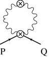
Figure 11: Possible contribution from the fermion-pair-2-gauge boson HTL vertex function to the HTL resummed DS equation for the fermion self-energy function $\Sigma_{R}$. $\bigotimes$ denotes the corresponding vertex function and propagator being the HTL resummed ones.

ii) There are no contributions from the fermion-pair-2-gluon vertex function in Eq.(V.1). In QCD this happens quite miraculously, namely the contribution to $\Sigma_{R}$ from the diagrams shown in Fig.11 are totally and exactly accounted for through the loop diagram with two 3-point quark-gluon vertices in Eq.(V.1). Inclusion of the contribution from Fig.11 causes the trouble of double counting of diagrams.

iii) The first term in the curly bracket, which exists also in the limit of ladder approximation, has been dismissed in previous DS equation analyses 13 . As can be seen this term could produce an dominant contribution due to the presence of the enhanced temperature dependence. Result of the analysis of Eq.(V.1) will be given elsewhere 17 .

Similarly we can write down the DS equation for the gauge boson polarization tensor, with which the full QCD analysis may be performed. In the DS equation for the gluon polarization tensor, which is not given here explicitly, the contribution from the gluon 4-point vertex does exist. However, in this case also contributions from the HTL’s, $\delta\Gamma^{\mu\nu\rho\sigma}$, Eqs.(III.24), are totally and exactly accounted for through the loop diagram with two 3-point gluon vertices, thus to avoid the double counting problem only the contribution from the tree 3-gluon vertex survives. Results of the analysis including the DS equation for the gauge boson polarization tensor itself will also be presented elsewhere 17 .

VI Conclusions and Discussion

In this paper we calculated the $n$-point HTL vertex functions in QCD/QED for $n$= 2, 3 and 4 in the physical representation in the RTF. The result showed that the $n$-point HTL vertex functions can be classified into two groups, a) those with odd numbers of external retarded indices, and b) the others with even numbers of external retarded indices. The $n$-point HTL vertex functions with one retarded index, which obviously belong to the first group a), are nothing but the HTL vertex functions that appear in the ITF, and vise versa 6 . All the HTL vertex functions belonging to the first group a) are of $O(g^{2}T^{2})$ , and satisfy among them the simple QED-type Ward-Takahashi identities, as in the ITF 1 ; 2 . All the HTL vertex functions with a fermion pair belong to this first group a). Those vertex functions belonging to the second group b) never appear in the ITF, namely their existence is characteristic of the RTF, and their HTL’s have the high temperature behavior of $O(g^{2}T^{3})$, one-power of $T$ higher than usual. Despite of this difference we could verify that those HTL vertex functions belonging to the second group b) also satisfy among themselves the QED-type Ward-Takahashi identities, thus guaranteeing the gauge invariance of the HTL’s in the real time thermal QCD/QED. The group b) HTL’s consist of the $n$-gluon vertex functions.

Comments and discussion are in order.

i) With the present results we can feel at ease to perform in the framework of real time thermal field theories the nonperturbative analyses in the HTL approximation on dynamical phenomena such as the chiral phase transition. As an application we derived the HTL resummed DS equation for the retarded fermion self-energy function, enabling us to study in QCD/QED the chiral phase transition at finite temperature, which is now under investigation 17 .

ii) It is well known that all the HTL contribution in the ITF are of order $O(g^{2}T^{2})$. Are there anything wrong in our results, Eqs. (III.8c), (LABEL:3.18e-g), and (III.24e-g), contradicting to the previous results? The answer is NO. It is shown 6 that the $n$-point functions in the ITF is nothing but the special combination of those in the RTF, namely, just the $n$-point functions in the real time physical representation with only one external retarded index, all the other ($n$-1) external indices being the advanced ones. This means that the $n$-point functions with more than two external retarded indices never have their counterparts in the ITF. Furthermore we have already had some results indicating the existence of the order $O(g^{2}T^{3})$ contributions in the RTF 8 ; 9 . Our results as above have clearly shown that such order $O(g^{2}T^{3})$ contributions really exist in the real time physical representation. Of course these unusual HTL’s appear only in the $n$-gluon vertex functions in QCD. In QED there are no 3-photon vertex functions and no 4-photon HTL vertex functions, as already shown.

iii) Another point to be noted is that the results, say, Eqs. (III.8a-c) have nothing in trouble with the number of independent components which is in the present case only one. As we can easily see the HTL contributions satisfy Eq.(III.2a),

$$\delta\Pi^{\mu\nu}_{AR}(P,Q)=(\delta\Pi^{\mu\nu}_{RA}(P,Q))^{*}.$$

Remembering that Eq.(III.2b) holds among the full two point vertex functions and here we are studying the HTL contributions, we can see that the additional power of $T$ in Eq.(III.6c) comes from the boson distribution function, guaranteeing the number of independent components in the present case being only one. The same is true for 3- and 4-point vertex functions with more than two external retarded indices.

iv) As noticed at the end of section IV, although the Ward-Takahashi identities (IV.2f) and (IV.3g), and also those (IV.5e) and (IV.5f) seem to have a bit different structure from others in Eqs.(IV.2), (IV.3) and (IV.5), all the identities (IV.2a-g), (IV.3a-g) and (IV.5a-g) actually have the same structure. This fact can be clearly seen by noticing that, e.g., the right-hand-sides of Eqs. (IV.5e) and (IV.5f) are the HTL contributions to the $\{RR\}$-component of gluon polarization tensor which is actually the difference of two polarization tensors,

$$\Pi^{\mu\nu}_{RR}(P,Q)=(1-2n_{B}(q_{0}))\mbox{sgn}(q_{0})(\Pi^{\mu\nu}_{RA}(P,Q)-\Pi^{\mu\nu}_{AR}(P,Q)),\ \ P+Q=0,$$ (VI.1)

namely, in the HTL approximation (where the external momentum $-P=Q$ must be soft)

$$\delta\Pi^{\mu\nu}_{RR}(P,Q)\hat{=}\frac{2T}{q_{0}}(\delta\Pi^{\mu\nu}_{RA}(P,Q)-\delta\Pi^{\mu\nu}_{AR}(P,Q)).$$ (VI.2)

Eq.(VI.2) shows that the right-hand-sides of Eqs. (IV.5e) and (IV.5f) are nothing but the difference of two HTL gluon polarization tensors, thus having exactly the same structure as others. The same is true for the right-hand-sides of identities (IV.2f) and (IV.3g), though less clear but can be easily seen with explicit manipulations.

v) We showed explicitly that in the physical representation in the RTF there exist those vertex functions with two external retarded indices having the high temperature behavior of $O(g^{2}T^{3})$. This should be true for any $n$-gluon vertex functions with even number external retarded indices.

Figure 1: One-loop diagram for the fermion self-energy and the definition of its HTL, $\delta\Sigma$. $\hat{=}$ denotes the equality in the HTL approximation.

Figure 2: One-loop diagram for the gauge boson polarization tensor andthe definition of its HTL, $\delta\Pi^{\mu\nu}$. In QED only the diagram (a) exists.

Figure 3: Definition of the fermion-gauge boson HTL resummed vertex function $\ {}^{*}\Gamma^{\mu}$.

Figure 4: One-loop diagrams for the fermion-gauge boson vertex function. In QED only the diagram (a) exists.

Figure 5: Definition of the 3-gauge boson HTL resummed vertex function $\ {}^{*}\Gamma^{\mu\nu\rho}$.

Figure 6: One-loop diagrams for the 3-gauge boson vertex function. Figure (d) represents all possible diagrams with independent configuration with respect to the three external legs with momenta $P,\ Q$ and $R$.

Figure 7: Definition of the fermion-pair-2-gauge boson HTL resummed vertex function $\ {}^{*}\Gamma^{\mu\nu}.$

Figure 8: One-loop diagrams for the fermion-pair-2-gauge boson vertex function. Their possible exchanged diagrams between the external gauge boson legs with momenta $R$ and $S$ should also be added. In QED only the diagram (a) and its exchanged diagram exist.

Figure 9: Definition of the 4-gluon HTL resummed vertex function $\ {}^{*}\Gamma^{\mu\nu\rho\sigma}.$ Color indices of the external gluons with momenta $R$ and $S$ is summed over, which is indicated by the same color index $c$.

Figure 10: One-loop diagrams for the 4-gluon vertex function. For figures (a), (b) and (c), their possible exchanged diagrams among the external legs with momenta $Q,\ R$ and $S$ should also be added. Figures (d) and (e) represent all possible diagrams with independent configuration with respect to the four external legs with momenta $P,\ Q,\ R$ and $S$.

- (1) E. Braaten and R. D. Pisarski, Nucl. Phys. B337, 569 (1990); B339, 310 (1990).
- (2) J. Frenkel and J. C. Taylor, Nucl. Phys. B334, 199 (1990).
- (3) N. P. Landsman and Ch. G. van Weert, Phy. Rep. 145, 141 (1987); J. I. Kapusta, Finite Temperature Field Theory (Cambridge University Press, Cambridge, England, 1989); M. LeBellac, Thermal Field Theory (Cambridge University Press, Cambridge, England, 1996).
- (4) K.-C. Chou, Z.-B. Su, B.-L. Hao and L. Yu, Phys. Rep. 118, 1 (1985).
- (5) L. V. Keldysh, Zh. Eksp. Teor. Fiz. 47, 1515 (1964) [Sov. Phys. JETP 20, 1018 (1965)].
- (6) T. S. Evans, Nucl. Phys. B347, 329(1992).
- (7) Hou Defu, M. E. Carrington, R. Kobes, and U. Heinz, Phys. Rev. D61 085013 (2000).
- (8) J. C. Taylor, Phys. Rev. D48, 958 (1993).
- (9) Defu et al 7 calculated the four-point HTL vertex functions in QED. Unfortunately, however, their results on the two-fermion-two-gauge-boson (photon) HTL vertex function with two retarded indices (as for the definition, see below) are not correct.
- (10) H. Nakkagawa, A. Niégawa and H. Yokota, Phys. Lett. B244, 63 (1990); Phys. Rev. D44, 473 (1991).
- (11) Our notations are the same as those used in Ref.7 , being slightly different from the originalones in Ref.4 . Details of the definitions and notations are given in section II.
- (12) This result differs from the one in Ref.7 , in which it is claimed that there exist the non-vanishing HTL contributions in the 2f-2g 4-point vertex functions with two retarded indices, being proportional to . The corresponding Ward-Takahashi identities they have claimed to hold are nothing but “0=0” in our case.
- (13) M. E. Carrington, and U. Heinz, Eur.Phys. J. C1,619 (1998).
- (14) Hou Defu, E. Wong, and U. Heinz, J. Phys. G24, 1861 (1998).
- (15) V. V. Klimov, Sov. J. Nucl. Phys. 33,934 (1981); Sov. Phys. JETP 55, 199 (1982); H. A. Weldon, Phys. Rev. D26, 1394 (1982); Phys. Rev. D26, 2789 (1982).
- (16) A. Barducci, R. Casalbuoni, S. De. Curtis, R. Gatto and G. Pettini, Phys. Rev. D41, 1610 (1990); S. K. Kang, W.-H. Kye and J. K. Kim, Phys. Lett. B299, 358 (1993); K.-I. Kondo and K. Yoshida, Int. J. Mod. Phys. A10, 199 (1995); M. Harada and A. Shibata, Phys. Rev. D59, 014010 (1999); K. Fukazawa, T. Inagaki, S. Mukaigawa and T. Muta, Prog. Theor. Phys. 105, 979 (2001).
- (17) E. Braaten and R. D. Pisarski, Phys. Rev. Lett. 64, 1338 (1990); Phys. Rev. D42, 2156(1990). See also, M. LeBellac, in Ref.[3].
- (18) R. Baier, H. Nakkagawa and A. Niégawa, Can. J. Phys. 71, 205 (1993); H. Nakkagawa, A. Niégawa and B. Pire, Phys. Lett. B294, 396 (1993); Can. J. Phys. 71, 269 (1993).
- (19) H. A. Weldon, Ann. Phys. (N.Y.) 271, 141 (1999).
- (20) Y. Fueki, H. Nakkagawa, H. Yokota and K. Yoshida, to appear.