Abstract

We update the determination of $|V_{us}|$ using semielectronic and semimuonic decays of $K$ mesons. A modest improvement of 15% with respect to its present value is obtained for the error bar of this matrix element when we combine the four available semileptonic decays. The combined effects of long-distance radiative corrections and nonlinear terms in the vector form factors can decrease the value of $|V_{us}|$ by up to 1%. Refined measurements of the decay widths and slope form factors in the semimuonic modes and a more accurate calculation of vector form factors at zero momentum transfer can push the determination of $|V_{us}|$ at a few of percent level.

PACS: 12.15.Hh, 13.20.Eb, 11.30.Hv,13.40.Ks

1. Introduction

$V_{ud}$ and $V_{us}$ are the most accurate entries of the Cabibbo-Kobayashi-Maskawa (CKM) matrix [1] that have been determined up to now. Their values recommended by the Particle Data Group are [2]:

$$|V_{ud}| = 0.9735\pm 0.0008\ ,$$ (1)

$$|V_{us}| = 0.2196\pm 0.0023\ .$$ (2)

When they are combined with $|V_{ub}|=0.0036\pm 0.0010$ [2], the most precise test of the unitarity condition of the CKM matrix up to date becomes:

$$|V_{ud}|^{2}+|V_{us}|^{2}+|V_{ub}|^{2}=0.9959\pm 0.0019\ .$$ (3)

Neither the central value nor the error bar quoted for $|V_{ub}|$ play any role in the present test of this unitarity condition. The error bars quoted in Eq. (1) for $V_{ud}$ and $V_{us}$ contribute to 70% and 30% of the total uncertainty in Eq. (3), respectively. A direct inspection of Eq. (3) would indicate that the present experimental values for these entries of the CKM matrix, fail to satisfy unitarity by 2.2$\sigma$. This problem makes necessary that further efforts are devoted to investigate the sources of uncertainties that play a role in the determination of $V_{ud}$ and $V_{us}$ [3] at the level of $10^{-4}$ and $10^{-3}$, respectively.

The value quoted for $V_{ud}$ in Eq. (1) arises [2] from the average of their values extracted from Superallowed Fermi Transitions (SFT) in nuclei and from free neutron beta decay. At present, the error bar in $V_{ud}$ from SFT is still dominated by different model-dependent calculations of isospin breaking corrections [4]; despite the fact that isospin breaking corrections in individual SFT’s are at a few times $10^{-3}$ level, the resulting uncertainty in the weighted average for $V_{ud}$ is small (5$\times 10^{-4}$!) [4] because a large set of 9 decays are used in their determination. On the other hand, the determination of $V_{ud}$ from neutron beta decay is reaching the $10^{-3}$ accuracy due to recent improvements in the measurements of the neutron lifetime [5] and the ratio of its vector and axial couplings [6]. We have recently reviewed [7] this determination of $V_{ud}$ by putting careful attention to the sources of uncertainties in the neutron decay rate at the $10^{-4}$ level. It was concluded [7] that present inconsistencies among the measurements of the axial-vector form factor $g_{A}(0)$ [6] are behind the main limitations in order to have an alternative accurate determination of $V_{ud}$.

In the present paper, we focus on the determination of $V_{us}$ from kaon semileptonic decays. The value quoted in Eq. (2), was determined in 1984 by Leutwyler and Roos [9] using kaon semielectronic decays: $K\rightarrow\pi e\nu_{e}$ ($K_{e3}$). Several articles (see for example [11, 12]) and comprehensive review papers have appeared [13, 14] that make different updates to the value of $|V_{us}|$ reported in [9]. Some of them (see for example ref. [13]), however, combine old data for the integrated spectra (those of ref [9]) with new information on the decay widths of $K_{e3}$. Since new information on the decay widths and form factors of $K_{e3}$ decays has been accumulated since Leutwyler and Roos’ original work (which is based in Ref. [10]), we would like in this paper to explore their impact in the determination of $V_{us}$. In addition, in the present paper we also include in our analysis the data corresponding to kaon semimuonic decays ($K_{\mu 3}$). We paid particular attention to the effects of long-distance radiative corrections in the and of non-linearities in the squared momentum-transfer dependence of the form factors in the extraction of $|V_{us}|$. It is found that those combined effects can decrease the central value of $|V_{us}|$ by up to 1%. We are not able to sensibly improve the accuracy in the determination of $V_{us}$ with respect to Eq. (2), but we can identify some elements of the analysis that, if improved, will help to obtain a more refined and consistent value of this CKM matrix element.

2. Decay amplitude and form factors

Let us start by defining the tree-level decay amplitude for the $K(p)\rightarrow\pi(p^{\prime})l^{+}(p_{1})\nu_{l}(p_{2})$ ($K_{l3}$, with $l=e,\mu$) decays [15]:

$${\cal M}=\frac{G}{\sqrt{2}}V_{us}C_{K}\langle\pi(p^{\prime})|\bar{u}\gamma_{\mu}s|K(p)\rangle\bar{v}(p_{1})\gamma^{\mu}(1-\gamma_{5})u(p_{2})\ ,$$ (4)

where $V_{us}$ is the CKM matrix element we are interested in, $G$ is the effective weak coupling at the tree-level and $C_{K^{0}}=\sqrt{2}C_{K^{+}}=1$ are flavor isospin Clebsh-Gordan coefficients for the hadronic matrix elements. The properties of the hadronic matrix elements have been discussed in numerous papers before (see for example [15]). Here we focus on some of their properties under flavour symmetry breaking that are relevant for the determination of $V_{us}$.

Using Lorentz covariance, we can write the hadronic matrix element as:

$$\langle\pi(p^{\prime})|\bar{u}\gamma_{\mu}s|K(p)\rangle=f_{+}(t)\left((p+p^{\prime})_{\mu}-\frac{m_{K}^{2}-m_{\pi}^{2}}{t}q_{\mu}\right)+f_{0}(t)q_{\mu}\left(\frac{m_{K}^{2}-m_{\pi}^{2}}{t}\right)\ .$$ (5)

The form factors $f_{+,0}$ are Lorentz-invariant functions of the squared momentum transfer ($t=q^{2}=(p-p^{\prime})^{2}$). They correspond to the $l=1,0$ angular momentum configuration of the $K-\pi$ system in the crossed channel, respectively. The kinematical range allowed for the squared momentum transfer in $K_{l3}$ decays is $m_{l}^{2}\leq t\leq(m_{K}-m_{\pi})^{2}$. The analiticity of the amplitude for low values of $t$ demands that $f_{0}(0)=f_{+}(0)$.

In the limit of exact isospin symmetry, we have ($i=+$ or $0$):

$$f^{K^{+}\rightarrow\pi^{0}}_{i}(t)=f^{K^{0}\rightarrow\pi^{-}}_{i}(t).$$ (6)

This means that the form factors of charged and neutral $K$ mesons should be equal for all values of $t$ in this limit. If we rewrite the form factors as follows

$$f_{i}(t)=f_{i}(0)\tilde{f}_{i}(t)$$ (7)

we have $\tilde{f}_{i}(0)=1$. Thus, isospin symmetry would imply:

$$f^{K^{+}\rightarrow\pi^{0}}_{+}(0)=f^{K^{0}\rightarrow\pi^{-}}_{+}(0)\ ,$$

and, for all values of $t$:

$$\tilde{f}^{K^{+}\rightarrow\pi^{0}}_{i}(t)=\tilde{f}^{K^{0}\rightarrow\pi^{-}}_{i}(t)\ .$$ (8)

The effects of isospin and SU(3)-flavour symmetry breaking will modify these relations.

The form factors $\tilde{f}^{K\rightarrow\pi}_{+,0}(t)$ have been measured experimentally [2] for $K_{l3}$ decays. It has been found that a linear parametrization in $t$,

$$\tilde{f}^{K\rightarrow\pi}_{+,0}(t)=1+\frac{\lambda_{+,0}}{m_{\pi}^{2}}t\ ,$$ (9)

is sufficient to describe the data, in most of the kinematical range of $K_{l3}$ decays, to the degree of accuracy attained by experiments. Note that in Eq. (9), the mass scale in the denominator is set by the mass of the pion emitted in the corresponding $K$ decay. Thus, the isospin symmetry relation of Eq. (8) indicates that the dimensionful quantities $\lambda^{\prime}_{+,0}\equiv\lambda_{+,0}/m_{\pi}^{2}$ are the same for charged and neutral kaon decays.

For comparison, the experimental results for the slope constants $\lambda_{+,0}$ as used in the Leutwyler and Roos’ analyses [9] and in the present paper (using the data of Ref. [2]) are shown in Table 1. We observe that isospin violation in present data for $\lambda_{+}$ of $K_{e3}$ and $K_{\mu 3}$ decays are at a few percent level, as expected. However the average value reported for the $\lambda_{0}$ slopes in $K_{\mu 3}$ decays, strongly violates isospin symmetry [12]:

$$b_{0}=\frac{\lambda^{\prime}_{0}(K^{0}_{\mu 3})-\lambda^{\prime}_{0}(K^{+}_{\mu 3})}{\lambda^{\prime}_{0}(K^{0}_{\mu 3})+\lambda^{\prime}_{0}(K^{+}_{\mu 3})}=0.59\pm 0.37\ .$$ (10)

This large isospin breaking is usually thought to arise from the small value of $\lambda_{0}$ in $K_{\mu 3}^{+}$ decay. New high precision measurements of $K_{\mu 3}$ decays as those expected at Da$\phi$ne will be very useful to understand the nature of this isospin symmetry breaking effect. In this paper, we will use the values of $\lambda_{0}$ reported in ref. [2] and we will comment on the impact of the new result reported in ref. [16] on the determination of $V_{us}$.

Concerning the value of the form factor at $t=0$, we will use the values obtained in Ref. [9] (note however that our numerical results in sections 4.1–4.2 are obtained using $f_{+}^{K^{0}\rightarrow\pi^{-}}(0)=0.9606$, since the value of the $\pi^{-}$ decay constant used to evaluate the chiral corrections is now 0.8% smaller (see p. 395 in [2]) than the one used in [9]):

$$f_{+}^{K^{0}\rightarrow\pi^{-}}(0) = 0.961\pm 0.008\ ,$$ (11)

$$f_{+}^{K^{+}\rightarrow\pi^{0}}(0) = 0.982\pm 0.008\ .$$ (12)

These values exhibit an small isospin breaking effect:

$$r=\frac{f_{+}^{K^{+}\rightarrow\pi^{0}}(0)}{f_{+}^{K^{0}\rightarrow\pi^{-}}(0)}=1.022\ .$$ (13)

The form factors at $t=0$, Eqs. (11)–(12), incorporate the second order [19] SU(3) breaking effects arising from the $s-d,u$ quark mass difference and the isospin breaking corrections due to the $\pi^{0}-\eta$ mixing in the case of $f_{+}^{K^{+}\rightarrow\pi^{0}}(0)$ [9]. By including a full mixing scheme of neutral mesons $\pi^{0}-\eta-\eta^{\prime}$, one would obtain $r\approx 1.026$ [11], to be compared with Eq. (13). In sections 4.1-4.2, we quote within square brackets our corresponding results obtained using this additional isospin correction. The large error assigned to Eqs. (11,12) are, at present, the main source of uncertainty in the value reported in Eq. (2). Other calculations of these form factors have been done using either the relativistic constituent quark model [20] or in a formalism based on the Schwinger-Dyson equations [21]. Their results are fully consistent with the ones shown in Eqs. (11,12), but theoretical errors are not provided for them (Ref. [20] provides an error bar $\delta f_{+}^{K^{0}\rightarrow\pi^{-}}=^{+0.002}_{-0.006}$ associated to uncertainties in the strange quark mass). Thus, we will restrict ourselves to the results quoted in the previous equations.

The linear parametrizations of the form factors are a convenient although arbitrary choice to describe experimental data for all values of $t$ in $K_{l3}$ decays. On the other hand, information about these form factors can be obtained from $\tau\rightarrow K\pi\nu_{\tau}$ decays in the region $(m_{K}+m_{\pi})^{2}\leq t\leq m_{\tau}^{2}$. The vector form factors in $\tau$ decays display a resonant structure [22] such that when they are extrapolated to low values of $t$ they will naturally induce nonlinear terms. Following the results obtained in $\tau\rightarrow\pi\pi\nu_{\tau}$ decays, which suggest that two or more vector resonances dominate the 2$\pi$ mass distribution [23], one can model the vector form factor in $\tau\rightarrow K\pi\nu_{\tau}$ decays as follows [24]:

$$\tilde{f}_{+}(t)=\frac{1}{1+\beta_{K^{*}}}[BW_{K^{*}}(t)+\beta_{K^{*}}BW_{K^{\prime*}}(t)]\ ,$$ (14)

where

$$BW_{X}(t)=\frac{m_{X}^{2}}{m_{X}^{2}-t-i\sqrt{t}\Gamma_{X}(t)\theta(t-(m_{K}+m_{\pi})^{2})}\ .$$

The subindex $X=K^{*}(892),K^{\prime*}(1410)$ denote the charged vector resonances in the $l=1$ configuration of the $K\pi$ system, $\Gamma_{X}(t)$ is the corresponding decay width and $\beta_{K^{*}}$ is used to denote the relative strength of both contributions.

When we extrapolate Eq. (14) below the $K\pi$ threshold, we obtain:

$$\tilde{f}_{+}(t)=\frac{1}{1+\beta_{K^{*}}}\left[\frac{m_{K^{*}}^{2}}{m_{K^{*}}^{2}-t}+\beta_{K^{*}}\frac{m_{K^{\prime*}}^{2}}{m_{K^{\prime*}}^{2}-t}\right].$$ (15)

If we set $\beta_{K^{*}}=0$, and expand the resulting form factor in powers of $t$, one obtains $\lambda_{+}=(m_{\pi}/m_{K^{*}})^{2}=0.024$. The fact that a single pole $K^{*}(892)$ underestimates the value of $\lambda_{+}$ was discussed long ago (see for example ref. [25]). Now, when we expand this expression up to terms of order $t$, we can find the value of the free parameter $\beta_{K^{*}}$ from the values of $\lambda_{+}$ of each $K_{l3}$ decay according to:

$$\beta_{K^{*}}=-\left(\frac{\lambda_{+}-r_{K^{*}}}{\lambda_{+}-r_{K^{\prime*}}}\right)\ ,$$

where $r_{X}=(m_{\pi}/m_{X})^{2}$. Thus, the vector form factor with two poles given in Eq. (15) is a natural generalization that includes non-linear effects in $t$ and reproduces the correct size of the coefficients in the linear terms. An estimate of the effects of nonlinear terms in the determination of $|V_{us}|$ was given for example in ref. [12].

3. Decay rates and radiative corrections

When the radiative corrections are added to the lowest order amplitude, the decay rate of the $K_{l3}$ decays can be written as follows [9]:

$$\Gamma(K_{l3})=\frac{G_{F}^{2}m_{K}^{5}}{192\pi^{3}}S_{EW}C_{K}^{2}|f_{+}^{K\rightarrow\pi}(0).V_{us}|^{2}I_{K}(1+\delta_{K})\ ,$$ (16)

where $G_{F}=1.16639(1)\times 10^{-5}$ GeV^-2 [2] is the Fermi coupling constant obtained from $\mu$ decay, and the dimensionless integrated spectrum $I_{K}$ is defined as:

$$I_{K} = \frac{1}{m_{K}^{8}}\int_{m_{l}^{2}}^{(m_{K}-m_{\pi})^{2}}\frac{dt}{t^{3}}(t-m_{l}^{2})^{2}\lambda^{1/2}(t,m_{K}^{2},m_{\pi}^{2})$$ (17)

$$\times\left\{\lambda(t,m_{K}^{2},m_{\pi}^{2})(2t+m_{l}^{2})|\tilde{f}_{+}(t)|^{2}+3m_{l}^{2}(m_{K}^{2}-m_{\pi}^{2})^{2}|\tilde{f}_{0}(t)|^{2}\right\},$$

where $\lambda(x,y,z)\equiv x^{2}+y^{2}+z^{2}-2xy-2xz-2yz$. The second term in $I_{K}$ (proportional to $m_{l}^{2}$) shows that $K_{\mu 3}$ decays are more sensitive to the effects of the scalar form factor than $K_{e3}$ decays. In practice, the factor $(m_{K}^{2}-m_{\pi}^{2})^{2}$ in front of the scalar form factor provides a further suppression for this contribution. This fact helps our purposes of using $K_{\mu 3}$ decays in our analysis, because the issue of the isospin breaking in $\lambda_{0}$ discussed in the previous section is not very critical at the present level of accuracy to determine $V_{us}$.

As usual, in the above expression for the decay width we have factorized the radiative corrections into a short-distance electroweak piece $S_{EW}$, and a long-distance model-dependent QED correction $\delta_{K}$. Since energetic virtual gauge bosons explore the hadronic transitions at the quark level, $S_{EW}$ is, in good approximation, the same for all the $K_{l3}$ decays ; by including the resummation of the dominant logarithmic terms one obtains $S_{EW}=1.022$ [26].

The long distance radiative corrections $\delta_{K}$ are different for each process since they depend upon the charges and masses of the particles involved in a given decay. They were computed long ago for different observables associated to $K_{l3}$ decays [27] using the following approximations: $(i)$ point electromagnetic vertices of the pseudoscalar mesons, $(ii)$ fixed values of the hadronic weak form factors, and $(iii)$ the local four-fermion weak interaction. The values of $\delta_{K}$ for each of the four $K_{l3}$ decays [27] are shown in the last column of Table 1. It is interesting to observe that $\delta_{K}(K^{0}_{l3})-\delta_{K}(K^{+}_{l3})\approx 2\%$, both for semielectronic and semimuonic kaon decays. The origin of this difference can be traced back to the coulombic interaction between the pion and the charged lepton in $K^{0}_{l3}$ decays [27] (see also [11]). We discuss in section 4.2 the impact of these long-distance radiative corrections in the determination of $V_{us}$.

4. Determination of $V_{us}$

In this section we extract the quantities $|f_{+}(0).V_{us}|$ for each decay and provide a determination of $|V_{us}|$. We first ignore the effects of long-distance radiative corrections in order to compare our results with the ones provided in ref. [9]. Later we evaluate the effects of those radiative corrections and comment on the prospects to improve the accuracy in the determination of $V_{us}$ (see also refs. [12, 11].

4.1 $|V_{us}|$ without using radiative corrections

Using the input data of Table 1 and the decay rate of Eq. (16), we obtain the values for the integrated spectrum $I_{K}$ and the product $|f_{+}(0)V_{us}|$ shown in the second and third columns of Table 2, respectively. The error bars quoted for the latter quantities include a 1% uncertainty attributed to long-distance radiative corrections according to the prescription of ref. [9]. It is interesting to observe that the values of $|f_{+}^{K^{+}\rightarrow\pi^{0}}(0)V_{us}|$ obtained from $K^{+}_{e3}$ and $K^{+}_{\mu 3}$ decays are remarkably consistent among them as demanded by $e-\mu$ universality, despite the fact that isospin symmetry is strongly broken in the slope of the scalar form factor. The same can be stated (within errors) for the corresponding quantities in neutral kaon decays. Contrary to ref. [9], we have used the experimental values for the slopes of the form factors in $K_{e3}$ decays instead of assuming isospin symmetry (namely, we have not assumed $\lambda_{+}(K^{+}_{l3})=\lambda_{+}(K^{0}_{l3})$ as in [9]). Observe in Table 2 that the value of $|f_{+}(0)V_{us}|$ extracted from $K^{+}_{e3}$ is almost at the same level of accuracy than in $K^{0}_{e3}$.

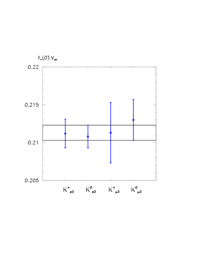
Figure 1: Values of $|f_{+}^{K^{0}\rightarrow\pi^{-}}(0).V_{us}|$ obtained from all $K_{l3}$ decays by ignoring long-distance radiative corrections. The horizontal band is the 1$\sigma$ weighted average of the four values.

Now, if we include the isospin breaking corrections to the form factors at $t=0$ using Eq. (13), we can express the results in Table 2 in terms of the quantity $|f_{+}^{K^{0}\rightarrow\pi^{-}}(0)V_{us}|$ from the four $K_{l3}$ decays. The different values of this quantity can be used as a consistency test of the calculations of the different corrections applied to the semileptonic decays, namely, this quantity must be the same for all $K_{l3}$ decays. In Fig. 1, we plot the values of $|f_{+}^{K^{0}\rightarrow\pi^{-}}(0)V_{us}|$ obtained from the four semileptonic kaon decays. We observe that their values are consistent among themselves and with their weighted average

$$|f_{+}^{K^{0}\rightarrow\pi^{-}}(0)V_{us}|=0.2113\pm 0.0010\ [0.2110\pm 0.0010],$$ (18)

which is displayed as an horizontal band in Fig. 1 (for $r=1.022$). In the previous equation and in the results of this and the following sections, we show within square brackets the figures corresponding to the choice $r=1.026$ of the isospin breaking correction (see discussion after eq. (13)). The scale factor (see p. 11 of ref. [2]) associated to the set of 4 independent measurements of $|f_{+}^{K^{0}\rightarrow\pi^{-}}(0)V_{us}|$ is $S=0.41$, indicating a good consistency of those results.

From equations (11) and (18) we obtain the following value:

$$|V_{us}| = 0.2200\times\left(1\pm\sqrt{(0.0083)^{2}_{f_{+}(0)}+(0.0047)^{2}_{``exp"}}\right)$$ (19)

$$= 0.2200\pm 0.0021\ [0.2197\pm 0.0021],$$

where we have used quotation marks on the experimental error to indicate that they contain a 1% uncertainty associated to radiative corrections. The present uncertainty in $|V_{us}|$ is dominated (75%) by the theoretical uncertainty in the calculation of $f_{+}(0)$ [9]. Thus, any experimental effort aiming to improve the accuracy in measurements of the $K_{l3}$ properties, should be accompanied of an effort to reduce the error bars in the calculation of form factors at $t=0$.

4.2 $|V_{us}|$ including radiative corrections

Before we proceed to include the effects of long-distance radiative corrections in the rates of $K_{l3}$ decays, let us first discuss the effects of these corrections in the determination of the slope parameter $\lambda_{+}(K^{+}_{e3})$ from experiments.

If we use the set of measurements of $\lambda_{+}(K^{+}_{e3})$ reported in [2] and include the effects of radiative corrections in all of them, we obtain the weighted average $\lambda_{+}^{rc}=0.0285\pm 0.0019$ (namely, an increase of 2.5% with respect to its value in the third column of Table 1). However, if we evaluate the phase space factor with this corrected value of $\lambda_{+}^{rc}$ we obtain $I_{K}(K^{+}_{e3})=0.1607$ to be compared with 0.1603 (see Table 1). This is an effect of only 0.2%, indicating that attributing a 1% error bar to the decay rates (see footnote 5) due to effects of long-distance radiative corrections probably overestimates this uncertainty.

Thus, we proceed to include explicitly the effects of $\delta_{K}$ in the decay rate. Using the input data of Table 1 into Eq. (16), we obtain the values for the product $|f_{+}(0)V_{us}|$ shown in the fourth column of Table 2. Once we include the isospin breaking corrections in the $|f_{+}(0)|$ values for $K^{+}$ decays, we obtain the following weighted average value from the four $K_{l3}$ decays:

$$|f_{+}^{K^{0}\rightarrow\pi^{-}}(0)V_{us}|=0.2101\pm 0.0008\ [0.2099\pm 0.0008]\ .$$ (20)

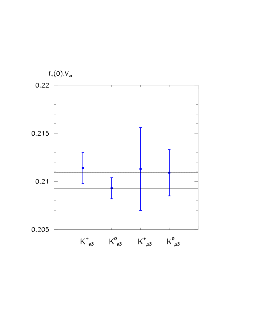
Figure 2: Same description as in Fig. 1 but when long-distance radiative corrections are included in the decay widths.

This quantity is plotted as an horizontal band in Fig. 2 (for $r=1.022$), together with the individual values obtained from the four kaon decays after including isospin breaking corrections from Eq. (13). The agreement among these four values is equally good (scale factor $S=0.66$) as in the case where long-distance radiative corrections were excluded (Fig. 1). Thus, on the basis of the scale factor alone we can conclude that the set of 4 measurements of the $|f_{+}^{K^{0}\rightarrow\pi^{-}}(0)V_{us}|$, obtained with and without radiative corrections, provide an equally consistent set of data.

Using the average value obtained in Eq. (20) we extract the CKM matrix element:

$$|V_{us}|_{rc} = 0.2187\times\left(1\pm\sqrt{(0.0083)^{2}_{f_{+}(0)}+(0.0038)^{2}_{exp}}\right)$$ (21)

$$= 0.2187\pm 0.0020\ [0.2185\pm 0.0020]\ ,$$

which is only 0.6% smaller than the value in Eq. (19). As in the case of section 4.1, the error bar is largely dominated by the uncertainty in the calculation of $f_{+}(0)$. For comparison, the corresponding value obtained from $K_{e3}$ decays alone is $|V_{us}|=0.2186\pm 0.0021\ [0.2183\pm 0.0020]$.

In summary, when we include long-distance radiative corrections in the decay rates, the value of $|V_{us}|$ decreases by almost 0.6% and the error bars remain almost the same. If we compare our result for $|V_{us}|$ in Eq. (21) with the one obtained in reference [9], Eq. (2), we observe that the overall uncertainty is being reduced by 15%. From Eqs. (19) and (21) we conclude that any experimental effort aiming to improve the precision in measurements of $K_{l3}$ properties would not have a significant impact on the determination of $|V_{us}|$. A reassessment of the SU(3) breaking effects in $f_{+}(0)$ is compelling to attain a greater accuracy in $|V_{us}|$.

However, an improvement in measurements of the properties of $K_{l3}$ decays would help to assess the requirement of long-distance radiative corrections. In particular, a consistency check of these calculations can be provided by verifying that the quantities $|f_{+}^{K^{0}\rightarrow\pi^{-}}(0)V_{us}|$ are the same in all four $K_{l3}$ decays. This quantity plays a similar role as the ${\cal F}t$ parameter in SFT, which must be the same for all the $0^{+}\rightarrow 0^{+}$ nuclear transitions after removing (process-dependent) isospin breaking and radiative corrections from the $ft$ value of each decay (see [4]).

4.3 Effects of non-linear form factors

In this section we study the effects on the determination of $|V_{us}|$ due to nonlinear terms that could be present in the vector form factors $f_{+}(t)$. These nonlinear terms are naturally induced when we extrapolate the vector form factor measured in the resonance region to energies below the threshold for $K\pi$ production (see discusion in section 2).

The strength $\beta_{K^{*}}$ of the relative contributions of the two resonances in the model of Eq. (15) can be fixed either, ($i$) from the slope of the $\tilde{f}_{+}(t)$ form factor at low momentum transfer or, ($ii$) from the decay rate of $\tau\rightarrow K\pi\nu$ decays. Using the first method, we can find the values of $\beta_{K^{*}}$ using the expression given after Eq. (15). The values obtained in this way are shown in the second column of Table 3. These values of $\beta_{K^{*}}$ are small and negative as expected from SU(3) symmetry considerations, since the corresponding parameter $\beta_{\rho}$ measured in $\tau\rightarrow\pi\pi\nu$ decays is also small and negative [23].

The corresponding integrated spectrum factor $I_{K}$ computed by using Eqs. (15) and (17) are shown in the third column of Table 3. A comparison of these results and the values of $I_{K}$ found for the linear case (second column in Table 2) indicates that in the nonlinear case, the values are shifted upwards by around 1% . Consequently, these nonlinearities in $t$ would decrease the individual values of $|f_{+}(0)V_{us}|$ (and of $|V_{us}|$) by an amount of 0.5% (see Table 4). Thus, instead of quoting a value of $|V_{us}|$ in this case, we would like to stress that nonlinear effects in the vector form factors of $K_{l3}$ decays would be very important in the precise determination of this CKM matrix element. In this case, more refined measurements of the this form factor both from the Dalitz plot or $\pi$ spectrum of $K_{l3}$ decays would be suitable.

5. Conclusions

In this paper we have used the updated information on semileptonic decay properties of kaons to determine the $|V_{us}|$ entry of the CKM mixing matrix. We have employed both, the semielectronic ($K_{e3}$) and semimuonic ($K_{\mu 3}$) decays of charged and neutral kaons. In addition to the original work of Ref. [9], we have explicitly included the effects of long-distance radiative corrections in our analysis and have studied the impact of non-linear vector form factors.

Our results are summarized in Table 4. We observe that the determination of $|V_{us}|$ from the semielectronic, the semimuonic and from the combined modes are consistent among them. The values of $|V_{us}|$ obtained from the muonic modes are larger than the ones obtained using the semielectronic modes, although they are less accurate. This difference becomes smaller when long-distance radiative corrections are included in the decay widths. On the other hand, long-distance radiative corrections tend to reduce the values of $|V_{us}|$ by a 0.3% (0.7%) in the electronic (muonic) channel. The error bars in the case of the semimuonic channels are still dominated by the experimental uncertainties in the decay widths and form factor slopes, while the corresponding error bars from the semielectronic modes are largely dominated by the theoretical uncertainty in the calculation of the form factors at zero momentum transfer. When we combine all the four $K_{l3}$ decay channels, we obtain a determination of $|V_{us}|$ which modestly improve the accuracy obtained by ref. [9], Eq. (2).

Concerning the effects of nonlinear form factors at low momentum transfer, we have considered a vector dominance model with two resonances, which turns out to be adequate in the resonance region. We fix the relative contributions of the two resonances by matching the form factor with experimental values at low energies. The overall effect of the nonlinear terms is to reduce the value of $|V_{us}|$ by a 0.5%. Thus, the combined effect of long-distance radiative corrections and nonlinear form factors could decrease the value of $|V_{us}|$ by up to 1%. New measurements of the vector form factors of $K_{l3}$ decays, particularly their energy dependence for soft pions (large values of the momentum transfer), will be very useful to improve the determination of $|V_{us}|$.

Finally, we would like to stress that the set of four kaon semileptonic decays turns out to be very useful to make a consistency test of the measurements and the different corrections applied to the decay rates. In particular, we mean that when isospin breaking corrections are removed from the vector form factors at zero momentum transfer, we can extract the product $|f_{+}^{K^{0}\rightarrow\pi^{-}}(0)V_{us}|$ which must be the same for all the four $K_{l3}$ decays. In other words, this parameter plays the same role as the process-independent ${\cal F}t$ values used in Superallowed Fermi nuclear Transitions to determine $|V_{ud}|$.

Acknowledgements The authors acknowledge the partial financial support from Conacyt (México) under contracts 32429-E and 35792-E.

Experiment	PDG 1982	PDG 2001	Ref. [27]
$K^{+}_{e3}$
$\Gamma$	2.5645$\pm$0.0271	2.5616 $\pm$ 0.0323
$\lambda_{+}$	0.029 $\pm$ 0.004	0.0278 $\pm$ 0.0019
$\delta_{K}$(%)	-	-	–0.45
$K^{0}_{e3}$
$\Gamma$	4.9147$\pm$0.0740	4.9385 $\pm$ 0.0446
$\lambda_{+}$	0.0300 $\pm$ 0.0016	0.0290 $\pm$ 0.0016
$\delta_{K}$(%)	-	-	1.5
$K^{+}_{\mu 3}$
$\Gamma$	1.7026$\pm$0.0480	1.6847 $\pm$ 0.0426
$\lambda_{+}$	0.026 $\pm$ 0.008	0.031 $\pm$ 0.008
$\lambda_{0}$	–0.003 $\pm$ 0.007	0.006 $\pm$ 0.007
$\delta_{K}$(%)	-	-	–0.06
$K^{0}_{\mu 3}$
$\Gamma$	3.4415 $\pm$ 0.0573	3.4604 $\pm$ 0.0416
$\lambda_{+}$	0.034 $\pm$ 0.006	0.034 $\pm$ 0.005
$\lambda_{0}$	0.020 $\pm$ 0.007	0.025 $\pm$ 0.006
$\delta_{K}$(%)	-	-	2.02

Table 1: Comparison of observables for $K_{l3}$ decays as reported by the Particle Data Group in 1982 (ref. [10]) and 2001 (ref. [2]). The decay widths $\Gamma$ are given in units of $10^{-15}$ MeV. The last column displays the long-distance radiative corrections to the decay widths according to Ref. [27].

Process	$I_{K}$	$|f_{+}(0)V_{us}|$ (worc)	$|f_{+}(0)V_{us}|$ (wrc)
$K^{+}_{e3}$	0.1603$\pm$0.0011	0.2158$\pm$0.0019	0.2160$\pm$0.0016
$K^{0}_{e3}$	0.1555$\pm$ 0.0008	0.2108$\pm$0.0015	0.2093$\pm$0.0011
$K^{+}_{\mu 3}$	0.1054$\pm$0.0033	0.2159$\pm$0.0041	0.2159$\pm$0.0043
$K^{0}_{\mu 3}$	0.1068$\pm$0.0021	0.2130$\pm$0.0027	0.2109$\pm$0.0024

Table 2: Integrated spectrum $I_{K}$ of $K_{l3}$ decays and values extracted for the product $|f_{+}(0)V_{us}|$ with (wrc) and without (worc) radiative corrections, using the input data from ref. [2].

Process	$\beta_{K^{*}}$	$I_{K}$	$|f_{+}(0)V_{us}|$ (worc)
$K^{+}_{e3}$	-0.1827	0.1616$\pm$0.0012	0.2149$\pm$0.0019
$K^{0}_{e3}$	-0.3057	0.1568$\pm$ 0.0009	0.2100$\pm$0.0016
$K^{+}_{\mu 3}$	-0.3060	0.1065$\pm$0.0049	0.2147$\pm$0.0054
$K^{0}_{\mu 3}$	-0.4454	0.1079$\pm$0.0032	0.2119$\pm$0.0036

Table 3: Integrated spectrum $I_{K}$ of $K_{l3}$ decays and values extracted for the product $|f_{+}(0)V_{us}|$ and without (worc) radiative corrections using the nonlinear form factors of Eq. (15).

$r$	Source	$|V_{us}|$ (without r.c.)	$|V_{us}|$ (with r.c.)	$|V_{us}|$ (without r.c.)
		linear f.f.	linear f.f.	nonlinear f.f.
	$K_{e3}$	0.2196 $\pm$ 0.0022	0.2186 $\pm$ 0.0021	0.2187 $\pm$ 0.0022
1.022	$K_{\mu 3}$	0.2212 $\pm$ 0.0030	0.2196 $\pm$ 0.0029	0.2200 $\pm$ 0.0036
	All decays	0.2200 $\pm$ 0.0021	0.2187 $\pm$ 0.0020	0.2189 $\pm$ 0.0021
	$K_{e3}$	0.2192$\pm$ 0.0022	0.2183 $\pm$ 0.0020	0.2184 $\pm$ 0.0022
1.026	$K_{\mu 3}$	0.2209 $\pm$ 0.0030	0.2194 $\pm$ 0.0029	0.2198 $\pm$ 0.0036
	All decays	0.2197 $\pm$ 0.0021	0.2185 $\pm$ 0.0020	0.2186 $\pm$ 0.0021

Table 4: Values of $|V_{us}|$ extracted for two values of the isospin-breaking parameter $r$ (see section 2), from different combinations of $K_{l3}$ decays and including (fourth column) or not (third column) the long-distance radiative corrections. Also shown are the values obtained using non-linear form factors but excluding rad. corrections (fifth column).

References

- [1] N. Cabibbo, Phys. Rev. Lett. 10, 351 (1963); M. Kobayashi and T. Maskawa, Prog. Theor. Phys. 49, 652 (1973).
- [2] D. E. Groom et al, Particle Data Group, Eur. Phys. Jour. C15, 1 (2000). See updated values at http://pdg.lbl.gov.
- [3] See for example: F. J. Gilman, Nucl. Inst. Meth. A462, 301 (2001); A. J. Buras, eprint hep-ph/0109197.
- [4] J. C. Hardy and I. S. Towner, eprints nucl-th/9812036 and nucl-th/9809087.
- [5] B. Mampe et al, JETPL 57, 82 (1993); J. Byrne et al, Europhysics Lett. 33, 187 (1996); S. Arzumanov et al, Nucl. Inst. Meth. A440, 511 (2000).
- [6] P. Bopp et al, Phys. Rev. Lett. 56, 919 (1986); B. Yerozolimnsky et al, Phys. Lett. B412, 240 (1997); H. Abele et al, Phys. Lett. 407, 212 (1997); P. Liaud et al, Nucl. Phys. A612, 53 (1997).
- [7] A. García, J. L. García-Luna and G. López Castro, Phys. Lett. B500, 66 (2001).
- [8] See for example: R. Flores-Mendieta, A. García and G. Sánchez-Colon, Phys. Rev. D54, 6855 (1996).
- [9] H. Leutwyler and M. Roos, Z. Phys. C25, 91 (1984).
- [10] M. Roos et al, Particle Data Group, Phys. Lett. B111, (1982).
- [11] G. López Castro and J. Pestieau, Mod. Phys. Lett. A4, 2237 (1989).
- [12] G. López Castro and G. Ordaz, Mod. Phys. Lett. A5, 755 (1990).
- [13] M. Bargiotti et al, Riv. Nuovo Cim. 23, 1 (2000) and references cited therein.
- [14] A. Höcker, H. Lacker, S. Laplace and F. Le Diberder, Eur. Phys. J. C21, 225 (2001) and references cited therein.
- [15] L. M. Chounet, J. M. Gaillard and M. K. Gaillard, Phys. Rep. 4, 199 (1972); Bailin, “Weak interactions” (Sussex University Press, 1977).
- [16] K. Horie et al, KEK-E246 Collaboration, Phys. Lett. B513, 311 (2001).
- [17] C. G. Callan and S. B. Treiman, Phys. Rev. Lett. 16, 153 (1966).
- [18] See for example: J. Bijnens, G. Colangelo, G. Ecker and J. Gasser in The Second Dane Physics Handbook, Eds. L. Maiani, G. Pancheri and N. Paver, p.315 (INFN, 1995).
- [19] M. Ademollo and R. Gatto, Phys. Rev. Lett. 13, 264 (1964).
- [20] W. Jaus, Phys. Rev. D44, 2851 (1991).
- [21] C.-R. Ji and P. Maris, Phys. Rev. D64, 014032 (2001)
- [22] R. Barate et al, ALEPH Collaboration, Eur. Phys. J. C10, 1 (1999).
- [23] R. Barate et al, ALEPH Collaboration, Z. Phys. . C76, 15 (1997); A. J. Weinstein et al, CLEO Collaboration, Nucl. Phys. Proc. Suppl. 98, 261 (2001).
- [24] J. Kühn and A. Santamaría, Z. Phys. C48, 445 (1990); M. Finkemeier and E. Mirkes, Z. Phys. C72, 619 (1996).
- [25] L. M. Sehgal, Proc. of the 1979 EPS Conf. on High Energy Physics, Geneva 1979; K. Yamada, Phys. Lett. B97, 156 (1980).
- [26] A. Sirlin and W. J. Marciano, Phys. Rev. Lett. 56, 22 (1986); ibid 61, 1825 (1988); A. Sirlin, Rev. Mod. Phys. 50, 573 (1978).
- [27] E. S. Ginsberg, Phys. Rev. 142, 1035 (1966); ibid 162, 1570 (1967); 171, 1675 (1968); D1, 229 (1970); Errata: Phys. Rev. 174, 2169 (1968); 187, 2281 (1969).
- [28] I. S. Towner, Nucl. Phys. A540, 478 (1992).