Cosmological magnetic fields induced by metric perturbations after inflation

Antonio L. Maroto

Physics Department, Stanford University
Stanford CA 94305-4060, USA

We consider the amplification of electromagnetic quantum vacuum fluctuations induced by the presence of metric perturbations at the end of inflation. We obtain the amplitude of the corresponding magnetic fields on super-Hubble scales and compare it with the requirements of the galactic dynamo mechanism for different values of the spectral index. Finally we discuss the possible effects of the dissipation of such fields in the form of gravitational waves.

PRESENTED AT

COSMO-01
Rovaniemi, Finland,
August 29 – September 4, 2001

1 Introduction

The origin of the large scale magnetic fields observed in galaxies and galaxy clusters still remains an open problem in astrophysics (see [1, 2] and references therein). Observations show that typical galactic fields have coherence lengths around $1-10$ kpc and strengths of $1$ $\mu$G. Magnetic fields in galaxy clusters are stronger $1-10$ $\mu$G, with larger coherence lengths $10-100$ kpc.

Although their origin is unknown, there are certain theoretical limits on their primordial strength. Thus, any homogeneous magnetic field existing before decoupling should be weaker than $B_{0}\leq 10^{-9}$ G in order to avoid the production of excessive anisotropies in the cosmic microwave background radiation [2, 3]. On the other hand, more recently [4], it has been shown that magnetic fields present before nucleosynthesis can be very efficiently dissipated in the form of gravity waves. The limits imposed by nucleosynthesis on the maximum allowed additional energy density in the form of gravity waves can be translated into limits on the primordial strength of magnetic fields. Those limits can be as stringent as $B_{0}\leq 10^{-39}$ G, for magnetic field generated during inflation with a thermal spectrum.

Concerning the origin of the fields, there are several mechanisms proposed in the literarature which can be roughly classified into two groups: first, magnetic fields can be produced by certain charge separation mechanisms during galaxy formation [5], or second, by the amplification of preexisiting seed fields. In the second case, the amplification can be achieved either by the adiabatic compression of the fields in the collapse of the protogalactic cloud, which requires a seed field of $B_{0}\sim 10^{-10}$ G; or by the galactic dynamo mechanism, where the differential rotation of the galaxy is able to transfer kinetic energy into magnetic field. In this last case, the limits on the primordial seed fields at decoupling are in the range [6] $B_{dec}\sim 10^{-17}-10^{-20}$ G for a flat universe without cosmological constant. For a flat universe with cosmological constant the limits are relaxed up to $B_{dec}\sim 10^{-25}-10^{-30}$ G. Concerning the generation of the neccesary seeds, there are also two main types of explanations. On one hand, those based on phase transitions in the early universe, whose main difficulty is that the typical field coherence length is very small. On the other hand, we have the amplification of electromagnetic (EM) quantum fluctuations during inflation [7]. The main problem in this case is that in order to get some amplification, it is necessary to break the conformal triviality of Maxwell equations in Friedmann-Robertson-Walker (FRW) backgrounds. Recently, we have have explored this possibility in [8], and in the present paper we review our main results. Let us then start by studying Maxwell equations in a cosmological background.

2 Maxwell equations in cosmological backgrounds

Consider Maxwell equations

$$\nabla_{\mu}F^{\mu\nu}=0,$$ (1)

in a Friedmann-Robertson-Walker background:

$$g^{0}_{\mu\nu}dx^{\mu}dx^{\nu}=a^{2}(\eta)(d\eta^{2}-\delta_{ij}dx^{i}dx^{j})$$ (2)

with the Coulomb gauge condition $\vec{\nabla}\cdot\vec{A}=0\Rightarrow A_{0}=0$.

The equation for the Fourier modes $A_{i}(\vec{q},\eta)$ is:

$$\frac{d^{2}}{d\eta^{2}}A_{i}(\vec{q},\eta)+q^{2}A_{i}(\vec{q},\eta)=0$$ (3)

The trivial solutions are given by positive and negative frequency plane-waves: $A_{i}(\vec{q},\eta)\propto e^{\pm iq\eta}$ which are valid $\forall\eta$. This implies that if we start at $\eta\rightarrow-\infty$ with a positive frequency plane-wave, we will end up in $\eta\rightarrow+\infty$ with the same kind of solution, i.e. there is no mixing between positive and negative frequency modes, and therefore there is no photon production. This is known as the conformal triviality of Maxwell equtions in FRW backgrounds.

Therefore, in order to get magnetic field amplification we need to break conformal invariance. There are several proposal in the literature, which in general require certain modifications of Maxwell electromagnetism [7, 9] or the introduction of new fields [10, 11]. Here we explore the alternative possibility, i.e. we will not modify Maxwell electromagnetism but the background metric, including scalar perturbations. This possibility is rather natural since we know that metric perturbations are present in our universe. Let us then consider the inhomogeneous background $g_{\mu\nu}=g^{0}_{\mu\nu}+h_{\mu\nu}$, where:

$$h_{\mu\nu}dx^{\mu}dx^{\nu}=2\Phi\;a^{2}(\eta)(d\eta^{2}+\delta_{ij}dx^{i}dx^{j})$$

is the most general form of the linearized scalar metric perturbations in the longitudinal gauge, where $\Phi(\eta,\vec{x})$ is the gauge-invariant gravitational potential.

Substituting this form of the metric into (1), we obtain the following linearized equations:

$$\frac{\partial}{\partial x^{i}}\left((1-2\Phi)(\partial_{i}A_{0}-\partial_{0}A_{i})\right) = 0,$$

$$\frac{\partial}{\partial\eta}\left((1-2\Phi)(\partial_{i}A_{0}-\partial_{0}A_{i})\right) + \frac{\partial}{\partial x^{j}}\left((1+2\Phi)(\partial_{j}A_{i}-\partial_{i}A_{j})\right)=0$$ (4)

Now, because of the presence of the inhomogeneous perturbations, plane waves are no longer exact solutions, and in principle we have the possibility of mode mixing, and as a consequence quantum vacuum fluctuations can be amplified. Particle production from inhomogeneous sources has been considered also in [12, 13]

3 Photon production

In order to define the asymptotic vacuum states, let us assume: $\Phi\rightarrow 0$ when $\eta\rightarrow\pm\infty$. This is a good approximation in the remote past, since the own metric perturbations are generated during inflation. It is also a good approximation in the asymptotic future for perturbations reentering the horizon right after inflation, since they oscillate with damped amplitude. As we will see later, these perturbations will give the leading contributions in our results.

Consider positive frequency plane-wave solution in the $in$ region:

$$A_{\mu}^{\vec{k},\lambda}(x,in)\smash{\mathop{\hbox to28.45274pt{\rightarrowfill}}\limits_{\eta\rightarrow-\infty}}A_{\mu}^{(0)\vec{k},\lambda}(x)=\frac{1}{\sqrt{2kV}}\epsilon_{\mu}(\vec{k},\lambda)e^{i(\vec{k}\vec{x}-k\eta)}$$ (5)

We are working in a box with finite comoving volume $V$ and the two physical polarization states satisfy: $\vec{\epsilon}(\vec{k},\lambda)\cdot\vec{k}=0$, $\epsilon_{0}(\vec{k},\lambda)=0$.

It is easy to see that in the $out$ region, the solution (5) will become a linear superposition of positive and negative frequency modes with different polarizations and different momenta.

$$A_{\mu}^{\vec{k},\lambda}(x,in)\smash{\mathop{\hbox to28.45274pt{\rightarrowfill}}\limits_{\eta\rightarrow+\infty}}\sum_{\lambda^{\prime}}\sum_{q}\left(\alpha_{kq\lambda\lambda^{\prime}}\frac{\epsilon_{\mu}(\vec{q},\lambda^{\prime})}{\sqrt{2qV}}e^{i(\vec{q}\vec{x}-q\eta)}+\beta_{kq\lambda\lambda^{\prime}}\frac{\epsilon_{\mu}^{*}(\vec{q},\lambda^{\prime})}{\sqrt{2qV}}e^{-i(\vec{q}\vec{x}-q\eta)}\right)$$ (6)

If we quantize these modes, we find for the creation and annihilation $out$ operators $a_{k\lambda}^{out\,\dagger}$, $a_{k\lambda}^{out}$ a similar expansion in terms of $in$ operators:

$$a_{k\lambda}^{out}=\sum_{\lambda^{\prime}}\sum_{q}\left(\alpha_{qk\lambda^{\prime}\lambda}a_{q\lambda^{\prime}}^{in}+\beta_{qk\lambda^{\prime}\lambda}^{*}a_{q\lambda^{\prime}}^{in\;\dagger}\right)$$ (7)

This implies that if we started in the remote past in the vacuum state $|0,in\rangle$, then the number of particles created in the $out$ region with momentum $k$ and polarization $\lambda$ will be given by:

$$\langle 0,in|N_{k\lambda}^{out}|0,in\rangle=\sum_{q}\sum_{\lambda^{\prime}}|\beta_{qk\lambda\lambda^{\prime}}|^{2}\neq 0$$ (8)

In order to obtain the total number of photons created by the perturbations, we need to know the value of the Bogolyubov coefficients $\beta_{qk\lambda\lambda^{\prime}}$, for that purpose we have to solve the equations of motion. Thus, we look for perturbative solutions in $\Phi$:

$$A_{\mu}^{\vec{k},\lambda}(x)=A_{\mu}^{(0)\vec{k},\lambda}(x)+A_{\mu}^{(1)\vec{k},\lambda}(x)+...$$ (9)

For the spatial equations in Fourier space we get up to first order [8]:

$$\frac{d^{2}}{d\eta^{2}}{A_{i}^{(1)\vec{k},\lambda}}(\vec{q},\eta)+q^{2}A_{i}^{(1)\vec{k},\lambda}(\vec{q},\eta)-J_{i}^{\vec{k},\lambda}(\vec{q},\eta)=0$$ (10)

where:

$$J_{i}^{\vec{k},\lambda}(\vec{q},\eta) = -\sqrt{\frac{2k}{V}}\left(\left(i\Phi^{\prime}(\vec{k}+\vec{q},\eta)+\frac{k^{2}-\vec{k}\cdot\vec{q}}{k}\Phi(\vec{k}+\vec{q},\eta)\right)\epsilon_{i}(\vec{k},\lambda)e^{-ik\eta}\right.$$

$$+ \left.(\vec{\epsilon}(\vec{k},\lambda)\cdot\vec{q})\;\Phi(\vec{k}+\vec{q},\eta)\frac{k_{i}}{k}e^{-ik\eta}-i\frac{\vec{\epsilon}(\vec{k},\lambda)\cdot\vec{q}}{q^{2}}\frac{d}{d\eta}\left(\Phi(\vec{k}+\vec{q},\eta)e^{-ik\eta}\right)q_{i}\right)$$

It is relatively easy to solve these equations up to first order in perturbations. The result is:

$$A_{i}^{\vec{k},\lambda}(\vec{q},\eta)=\frac{\epsilon_{i}(\vec{k},\lambda)}{\sqrt{2kV}}\delta(\vec{q}-\vec{k})e^{-ik\eta}+\frac{1}{q}\int_{\eta_{0}}^{\eta}J_{i}^{\vec{k},\lambda}(\vec{q},\eta^{\prime})\sin(q(\eta-\eta^{\prime}))d\eta^{\prime}$$ (12)

Comparing this solution with the expansion in (6), we get for the Bogolyubov coefficients:

$$\beta_{kq\lambda\lambda^{\prime}}=\frac{-i}{\sqrt{2qV}}\int_{\eta_{0}}^{\eta_{1}}\vec{\epsilon}\;(\vec{q},\lambda^{\prime})\cdot\vec{J}^{\;\vec{k},\lambda}(\vec{q},\eta)e^{-iq\eta}d\eta$$ (13)

where $\eta_{0}$ denotes the initial time of inflation and $\eta_{1}$ the present time.

In the inflationary cosmology, metric perturbations are generated when quantum fluctuations become super-Hubble sized during inflation and reenter the horizon during radiation or matter dominated eras as classical fluctuations. Therefore, we will consider only the effect of those super-Hubble scalar perturbations, whose evolution is given by [14]:

$$\Phi(\vec{k},\eta)=C_{k}\frac{1}{a}\frac{d}{d\eta}\left(\frac{1}{a}\int a^{2}d\eta\right)+D_{k}\frac{a^{\prime}}{a^{3}}\simeq C_{k}\,{\cal F}(\eta)$$ (14)

where the second term decreases during inflation and can be ignored. Introducing this form for the perturbations, we can obtain an explicit expression for the total number of photons created with momentum $k_{G}=2\pi/\lambda_{G}$ (corresponding to a galactic scale wavelength $\lambda_{G}\sim 10$ kpc), in terms of the power spectrum of metric perturbations. Thus we find:

$$N_{k_{G}}\simeq\frac{4(2\pi)^{3/2}}{3k_{G}}\int dk\,{\cal P}_{\Phi}(k)$$ (15)

where we have used $k\eta\ll 1$, which is valid for super-Hubble perturbations, and we have defined:

$${\cal P}_{\Phi}(k)=\frac{k^{3}|C_{k}|^{2}}{2\pi^{2}V}=A_{S}^{2}\left(\frac{k}{k_{C}}\right)^{n-1}$$ (16)

with $\lambda_{C}\simeq 3000\;\mbox{Mpc}$ and the COBE normalization $A_{S}\simeq 5\cdot 10^{-5}$. We have assumed a simple power-law behaviour for the power spectrum. Such behaviour should be valid up to some high-frequency cutoff $k_{max}$, corresponding to the perturbation with smallest wavelength produced during inflation. Typically that wavelength is related to size of the horizon at the end of inflation, and is given by $k_{max}\sim a_{I}H_{I}$.

4 Magnetic field generation

In order to relate the number of photons created with the magnetic field strength, we notice that very long wavelength photons can be seen as static electric or magnetic fields [7]. Because of the high conductivity of the universe during the radiation dominated era, the electric field components are damped very fast, whereas magnetic flux is conserved, i.e. $Ba^{2}=$const.

Thus, the energy density in a magnetic field mode $B_{k}$ will be given by:

$$\rho_{B}(\omega)=\omega\frac{d\rho_{B}}{d\omega}=\frac{|B_{k}|^{2}}{2}=w^{4}N_{k},$$ (17)

where $w=k/a$ is the physical wavenumber. Using the result for the occupation number in (15), we obtain:

$$|B_{k_{G}}^{dec}|\simeq\frac{2^{3/2}(2\pi)^{3/4}\;A_{S}}{\sqrt{3n}\;a_{dec}^{2}}\;\frac{k_{max}^{n/2}\;k_{G}^{3/2}}{k_{C}^{(n-1)/2}}$$ (18)

From this expression we see that the magnetic field spectrum is thermal, i.e., $B_{k}\sim k^{3/2}$. In order to compare this result with observations and with the limits imposed by the galactic dynamo mechanism, we have plotted in Fig.1 the magnetic field strength at decoupling versus the cut-off frequency $k_{max}$, for different values of the spectral index $n$. In general, the results are several orders of magnitude below the observed strengths. The dashed horizontal line represents the weakest field required to seed a galactic dynamo, corresponding to a flat universe with cosmological constant $\Omega_{\Lambda}=0.7$, $\Omega_{m}=0.3$ and $h=0.5$ [6].

In order to estimate the value of $k_{max}$ in typical models of inflation, let us assume $k_{max}\sim a_{I}H_{I}$, where the $I$ subindex denotes the end of inflation. For a model with $H_{I}=10^{13}$ GeV, we can estimate $a_{I}$ assuming that reheating is very efficient, so that all the energy density in the inflaton field is instantaneously converted into radiation with a temperature $T_{R}$. In this case, we have:

$$k_{max}\sim a_{I}H_{I}\sim\frac{a_{dec}T_{dec}H_{I}}{T_{RH}}$$ (19)

where we have assumed adiabatic evolution of the universe after reheating. For a typical reheating temperature $T_{R}\sim 10^{15}$ GeV, we have $k_{max}/k_{C}\simeq 10^{26}$, the corresponding magnetic field from Fig. 1 is below the requirements of the galactic dynamo. Only very large values of the cutoff frequency can give rise to a sufficiently strong seed magnetic field.

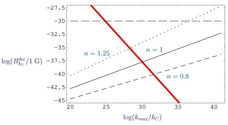
Figure 1: Magnetic field strength at decoupling on a galactic scale $k_{G}$ versus cut-off frequency $k_{max}$ for different values of the spectral index $n$. The continuous line corresponds to the scale-invariant Harrison-Zeldovich spectrum with $n=1$, the dashed line to $n=0.8$ and the dotted one to $n=1.25$. The dashed horizontal line corresponds to the weakest field required to seed a galactic dynamo, and the thick line is the limit imposed by gravity waves production given by (20).

5 Damping of magnetic field into gravity waves

Finally we will comment on the possible dissipation of magnetic fields in the form of gravity waves [4]. It is well-known that the interaction with the cosmic plasma is responsible for the damping of the magnetic field at small scales due to viscosity. However, if magnetic field are produced at very early times, the main dissipation mechanism is in the form of gravity waves [4], which are not damped by viscosity since they couple very weakly to matter. In that work, it has been shown that, in order to avoid an excess of energy density in gravity waves, that could modify the expansion rate of the universe during nucleosyntheis, the strength of any stochastic magnetic field created before nucleosynthesis should satisfy:

$$B_{k}<7\cdot 10^{-7}(\eta_{in}k)^{(n_{B}+3)/2}h_{0}\,{\cal N}(n_{B})\;{\mbox{G}}$$ (20)

where $B_{k}$ is the magnetic field mode strength (rescaled today) with momentum $k$, ${\cal N}(n_{B})\sim 1$, $\eta_{in}=1/k_{max}$ and $n_{B}$ is the magnetic field spectral index defined as $B_{k}^{2}\propto k^{n_{B}+3}$. Notice that for a thermal spectrum $n_{B}=0$. In Fig. 1, we have plotted the above limit (thick line) as a function of $k_{max}$ for the magnetic fields produced by metric perturbations whose spectral index is thermal, as shown before. We see that, such limit excludes the region of parameter space that could seed the galactic dynamo. However, still we can use these bounds to impose some limits on the primordial spectrum of metric perturbations at small scales. Thus, in order to avoid excessive gravity waves production (via magnetic fields), the cut-off frequency in the metric perturbations power spectrum should be $k_{max}/k_{C}<10^{30}$ for a scalar spectral index $n\simeq 1$.

6 Conclusions

In this paper, we have reviewed some of the results obtained in [8] concerning the production of large-scale magnetic fields from metric perturbations. We have shown how the breaking of conformal invariance induced by the presence of metric perturbations is able to produce photons at the end of inflation, and we have related the occupation number with the power spectrum of the metric perturbations.

We have compared the magnetic fields produced by this mechanism with the observations in galaxies and galaxy clusters and we have concluded that they are several order of magnitude weaker. Even with the assistance of galactic dynamo mechanism, only for extreme values of the parameters, this mechanism could explain the observations.

Finally, we have considered the dissipation of those magnetic fields in the form of gravity waves. Following the results in [4], we have shown that, like most of the models of magnetogenesis before nucleosynthesis, the one presented here would be excluded because of the excessive production of gravity waves. However, we can use the same limits on the primordial magnetic fields to impose certain bounds on the primordial spectrum of metric perturbations at small scales.

ACKNOWLEDGEMENTS

This work has been partially supported by the CICYT (Spain) projects AEN97-1693 and FPA2000-0956. The author also acknowledges support from the Universidad Complutense del Amo Fellowship.

References

- [1] P.P. Kronberg, Rep. Prog. Phys. 57, 325 (1994); E.N. Parker, Cosmical magnetic fields (Clarendon, Oxford) (1979); Y.B. Zeldovich, A.A. Ruzmaikin and D. Sokolov, Magnetic Fields in Astrophysics (Gordon and Breach, New York) (1983)
- [2] D. Grasso, H.R. Rubinstein Phys.Rept. 348 , 163 (2001)
- [3] J. Adams, U.H. Danielsson, D. Grasso and H. Rubinstein, Phys. Lett. B388, 253 (1996)
- [4] C. Caprini and R. Durrer, astro-ph/0106244
- [5] E.R. Harrison, Phys. Rev. Lett. 30 (1973) 188; R. M. Kulsrud, R. Cen, J.P. Ostriker and D. Ryu, Astrophys. J. 480 (1997) 481
- [6] A.C. Davis, M. Lilley and O. Törnkvist, Phys. Rev. D60 (1999) 021301
- [7] M.S. Turner and L.M. Widrow, Phys. Rev. D37 (1988) 2743
- [8] A.L. Maroto, Phys. Rev. D64 083006, (2001)
- [9] A.D. Dolgov, Phys. Rev. D48 (1993) 2499
- [10] B. Rathra, Astrophys. J. Lett. 391 (1992) L1
- [11] M. Gasperini, M. Giovannini and G. Veneziano, Phys. Rev. Lett. 75 (1995) 3796; E. Calzetta, A. Kandus and F. Mazzitelli, Phys. Rev. D57 (1998) 7139
- [12] J.A. Frieman, Phys. Rev. D39 (1989) 389; J. Céspedes and E. Verdaguer, Phys. Rev. D41 (1990) 1022
- [13] V. Zanchin, A. Maia, Jr., W. Craig and R. Brandenberger, Phys. Rev. D57 (1998) 4651 and D60 (1999) 023505; B.A. Bassett and S. Liberati, ibid. 58, 021302(R) (1998);B.A. Bassett, C. Gordon, R. Maartens and D.I. Kaiser, ibid 61, 061302(R) (2000)
- [14] V.F. Mukhanov, H.A. Feldman and R.H. Brandenberger, Phys. Rep. 215 (1992) 203
- [15] M. Giovannini and M. Shaposhnikov, Phys.Rev. D62 103512 (2000)