Non-adiabatic oscillations of supernova neutrinos

Abstract:

The level-crossing probability, local and global adiabaticity conditions are discussed for 2-flavour neutrino oscillations in matter with arbitrary mixing angles $\vartheta$. Different approximations for the survival probability of supernova neutrinos are compared. Results of a combined likelihood analysis of the observed SN 1987A neutrino signal and of the latest solar neutrino data including the recent SNO CC measurement are presented.

1 Neutrino evolution: resonance and adiabaticity conditions, maximal violation of adiabaticity

We consider neutrino oscillations in a two flavour scenario and label the heavier neutrino mass eigenstate with “2”. Then $\Delta=m_{2}^{2}-m_{1}^{2}$ is positive and the vacuum mixing angle $\vartheta$ is in the range $[0\!:\!\pi/2]$. As starting point for our discussion, we use the evolution equation for the medium states $\tilde{\psi}$ [1]

$$\frac{{\rm d}}{{\rm d}\vartheta_{\rm m}}\left(\begin{array}[]{c}\tilde{\psi}_{1}\\ \tilde{\psi}_{2}\end{array}\right)=\left(\begin{array}[]{cc}{{\rm i}}\frac{\Delta_{\rm m}}{4E\vartheta_{\rm m}^{\prime}}&-1\\ 1&-{{\rm i}}\frac{\Delta_{\rm m}}{4E\vartheta_{\rm m}^{\prime}}\end{array}\right)\left(\begin{array}[]{c}\tilde{\psi}_{1}\\ \tilde{\psi}_{2}\end{array}\right)\,,$$ (1)

where $\Delta_{\rm m}=\{\left(A-\Delta\cos 2\vartheta\right)^{2}+(\Delta\sin 2\vartheta)^{2}\}^{1/2}$ denotes the difference between the effective masses of the two (active) neutrino states in matter, $E$ is their energy and $A=2EV=2\sqrt{2}G_{F}N_{e}E$ is the induced mass squared for the electron neutrino. Furthermore, $\vartheta_{\rm m}$ is the mixing angle in matter and $\vartheta_{\rm m}^{\prime}={\rm d}\vartheta_{\rm m}/{\rm d}r$. Since anti-neutrinos feel a potential $V$ with the opposite sign than neutrinos, formulae derived below for neutrinos become valid for anti-neutrinos after the substitution $\vartheta\to\pi/2-\vartheta$.

The traditional condition for an adiabatic evolution of a neutrino state along a certain trajectory is that the diagonal entries of the Hamiltonian in Eq. (1) are large with respect to the non-diagonal ones, $|\Delta_{\rm m}|\gg|4E\vartheta_{\rm m}^{\prime}|$. This condition measures indeed how strong adiabaticity is locally violated. Therefore, the point of maximal violation of adiabaticity (PMVA) is given by the minimum of $\Delta_{\rm m}/\vartheta_{\rm m}^{\prime}$. In the following, we will concentrate on power-law like potential profiles, $A\propto r^{n}$. This type of profile does not only contain the case $n\approx-3$ typical for supernova envelopes, but also the exponential profile of the sun in the limit $n\to\pm\infty$. Moreover, it allows discussing which features of neutrino oscillations are generic and which ones are specific for the linear profile $n=1$ usually discussed. For $A(r)\propto r^{n}$, the minimum of $\Delta_{\rm m}/\vartheta_{\rm m}^{\prime}$ is at

$$\cot(2\vartheta_{\rm m}-2\vartheta)+2\cot(2\vartheta_{\rm m})$$ (2)

$$-\frac{1}{n}\,\left[\cot(2\vartheta_{\rm m}-2\vartheta)-\cot(2\vartheta_{\rm m})\right]=0\,.$$

For $n=1$, the PMVA is indeed at $\vartheta_{\rm m}=\pi/4$ for all $\vartheta$. Thus, in the region where the resonance point $\vartheta_{\rm m}=\pi/4$ is well-defined, they coincide. In the general case, $n\neq 1$, the PMVA agrees however only for $\vartheta=0$ with the resonance point.

In Fig. 1, we show the the change of the survival probability, ${\rm d}p(r)/{\rm d}r={\rm d}|\tilde{\psi}_{2}(r)|^{2}/{\rm d}r$ for a neutrino produced at $r=0$ as $\tilde{\nu}_{2}$, together with the PMVA predicted by Eq. (2) and the resonance point for a power law profile $A\propto r^{-3}$. The resonance condition predicts a transition in lower-density regions than the PMVA, until for $\vartheta=\pi/4$ the resonance point reaches $r=\infty$ and the concept of a resonant transition breaks down completely. Moreover, the crossing probability becomes less and less localized near the PMVA for larger mixing angles $\vartheta$.

Figure 1: Change of the survival probability ${\rm d}p(r)/{\rm d}r$ of a neutrino produced at $r=0$ as $\tilde{\nu}_{2}$ together with the point of maximal violation of adiabaticity (dot) and the resonance point (star) for a power law profile $A\propto r^{-3}$. The height of the different curves is rescaled.

Let us now discuss the condition for the adiabatic evolution of a neutrino state along a trajectory from the core of a star to the vacuum. While the condition $|\Delta_{\rm m}|\gg|4E\vartheta_{\rm m}^{\prime}|$ indicates whether adiabaticity is locally violated, we need now a global criterion that measures the cumulative non-adiabatic effects along the trajectory from $\vartheta_{\rm m}\approx\pi/2$ to $\vartheta$. For a non-adiabatic evolution of the neutrino state we require that

$$\bigg{|}\!\int_{\pi/2}^{\vartheta}{\rm d}\vartheta_{\rm m}\>\tilde{\psi}_{1}\bigg{|}=\varepsilon\>\bigg{|}\!\int_{\pi/2}^{\vartheta}{\rm d}\vartheta_{\rm m}\>\frac{4E\vartheta_{\rm m}^{\prime}}{\Delta_{\rm m}}\>\tilde{\psi}_{2}\bigg{|}$$ (3)

with $\varepsilon\ll 1$. Then the border between the adiabatic and non-adiabatic regions is given by

$$\frac{\Delta}{E}=\left\{\varepsilon\>\frac{f(\vartheta)}{\sin^{2}(2\vartheta)(1-\sin\vartheta)}\>\frac{2n(2V_{0})^{1/n}}{R_{0}}\right\}^{\frac{n}{n+1}}\,,$$ (4)

with

$$f(\vartheta) = |\int_{\pi/2}^{\vartheta}{\rm d}\vartheta_{\rm m}\sin\vartheta_{\rm m}\left[\sin(2\vartheta_{\rm m})\right]^{2+1/n}$$ (5)

$$\phantom{|\int_{\pi/2}^{\vartheta}}\times\left[\sin(2\vartheta_{\rm m}-2\vartheta)\right]^{1-1/n}|\,.$$

Fig. 2 shows the excellent agreement between our prediction for the border between the non-adiabatic and adiabatic regions for anti-neutrinos with energy $E=20$ MeV and a profile typical for supernova envelopes, $V(r)=1.5\times 10^{-9}$ eV $(10^{9}~{}{\rm cm}/r)^{3}$, and the one following from the contours of constant survival probability $P_{ee}$ (dashed lines) of the neutrino eigenstate $\tilde{\nu}_{2}$ obtained by solving the Schrödinger equation (1). A comparison of the solid ($n=-3$) and the dash-dotted line ($n\to\pm\infty$) shows moreover that $f(\vartheta)$ depends only weakly on $n$.

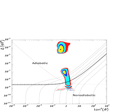
Figure 2: Contours of constant anti-neutrino survival probability (dashed) together with the borderline Eq. (4) between adiabatic and non-adiabatic regions using Eq. (5) with $n=-3$ (solid) and $n\to\pm\infty$ (dash-dotted) in $f(\vartheta)$ for the SN profile given in the text; the dotted line shows the borderline for neutrinos.

2 The crossing probability in the WKB formalism

The leading term to the crossing probability $P_{\rm LSZ}$ within the WKB formalism is in the ultra-relativistic limit and omitting an overall phase given by

$$\ln P_{\rm LSZ}=-\frac{1}{E}\>\Im\int_{x_{1}(A_{1})}^{x_{2}(A_{2})}{\rm d}x\>\Delta_{\rm m}\,,$$ (6)

where $A_{2}=\pm\Delta e^{2{{\rm i}}\vartheta}$ are the branch points of $\Delta_{\rm m}$ in the complex $x$ plane and and $x_{2}$ can be chosen arbitrarily either on the positive or negative real $x$ axis. The usual choice, $A_{1}=\Delta C$, allows to express $\ln P_{\rm LSZ}$ as the product of the adiabaticity parameter $\gamma$ evaluated at the resonance point and a correction function ${\cal F}_{n}$ [2] that can be represented as a hypergeometric function ${}_{2}F_{1}$ [3].

Another representation for the crossing probability which is valid for all $\vartheta$ uses as integration path in the complex $x$ plane the part of a circle of radius $\Delta$ centred at zero and starting from $A_{1}=\Delta$ and ending at $A_{2}=\Delta{\rm e}^{2{{\rm i}}\vartheta}$. For $A=A_{0}(r/R_{0})^{n}$, one can factor out the $\vartheta$ dependence of $P_{\rm LSZ}$ into functions ${\cal G}_{n}$ [3],

$$\ln P_{\rm LSZ}=-\kappa_{n}{\cal G}_{n}(\vartheta)\,,$$ (7)

where

$$\kappa_{n}=\left(\frac{\Delta}{E}\right)\>\left(\frac{\Delta}{A_{0}}\right)^{1/n}R_{0}$$ (8)

is independent of $\vartheta$ and

$${\cal G}_{n}(\vartheta)=\left|\;\Re\int_{0}^{2\vartheta/n}{\rm d}\varphi\>{\rm e}^{{{\rm i}}\varphi}\left[\left({\rm e}^{{{\rm i}}n\varphi}-C\right)^{2}+S\right]^{1/2}\right|$$ (9)

with $C=\cos 2\vartheta$ and $S=\sin 2\vartheta$.

3 Neutrino oscillations in supernova envelopes

In the analysis of neutrino oscillations, the potential profile $A(r)$ of supernova (SN) envelopes is often approximated by a power law with $n\approx-3$, and $V(r)=1.5\times 10^{-9}$ eV $(10^{9}~{}{\rm cm}/r)^{3}$. A comparison of the results of a numerical solution of the Schrödinger equation (1) with the analytical calculation of $P_{\bar{e}\bar{e}}$ using the ${\cal G}_{-3}$ functions shows very good agreement for this profile; only tiny deviations in the region $\Delta/(2E)\sim 10^{-17}$ eV have been found in [4]. By contrast, all other approximations used hitherto in the literature fail in some part of the $\tan^{2}\vartheta$–$\Delta$ plane: while the use of ${\cal F}_{1}=1$ together with $A\propto r^{-3}$ describes correctly the crossing probability for small mixing in the resonant region, the errors become larger for larger mixing until this approximation fails completely in the non-resonant region. The correction function ${\cal F}_{\infty}$ used for $n=-3$ describes quite accurately the most interesting region of large mixing as well as the non-resonant region, but does not reproduce the correct shape of the MSW triangle.

Figure 3: Comparison of the contours of constant survival probability $P_{\bar{e}\bar{e}}$ calculated numerically for a $M=20M_{\odot}$ progenitor star (dotted lines) and calculated for $A\propto r^{-3}$ with the $P_{\rm LSZ}$ approximation (solid lines).

More important is however to check how strong deviations of the true SN progenitor profile $V(r)$ from a power-law profile may affect the analytical results. Realistic progenitor profiles differ in two aspects from a simple $1/r^{3}$ behaviour. First, the outer part of the envelope has an onion like structure, and its chemical composition, $Y_{e}(r)$, and thus also $V(r)$ changes rather sharply at the boundaries of the various shells. Second, the density drops faster in the outermost part of the envelope, becoming closer to an exponential decrease. We calculated numerically $P_{\bar{e}\bar{e}}$ using profiles for different progenitor masses and stellar evolution models. We found that $P_{\bar{e}\bar{e}}$ is well approximated only in the non-resonant part by our analytical results for the $1/r^{3}$ profile, independently of the details of the progenitor profile, while $P_{\bar{e}\bar{e}}$ depends strongly on the details of the progenitor profile in the resonant region. As an example, we compare in Fig. 3 the $P_{\bar{e}\bar{e}}$ calculated numerically for a $20M_{\odot}$ profile with the analytical results for our standard SN profile. Therefore a numerical solution of the Schrödinger equation (1) should be performed in the resonant region, using a realistic profile for the particular progenitor star considered. However, a $1/r^{3}$ profile together with the WKB crossing probability is sufficient for the analysis of anti-neutrino oscillations in the phenomenologically most interesting region $\tan^{2}\vartheta\mathrel{\mathop{\kern 0.0pt\hbox to0.0pt{\raise 0.86108pt\hbox{$<$}\hss}}\lower 3.87495pt\hbox{\kern-1.90002pt$\sim$}}5$ independent of the details of the progenitor envelope.

Next we present the results of a combined statistical analysis of the neutrino signal of SN 1987A and of the complete set of solar neutrino experiments [4]. Since the two data sets are statistically independent and functions of the same two fit parameters, they can be trivially combined,

$$\chi^{2}_{\rm tot}(\vartheta,\Delta)=\chi^{2}_{\odot}(\vartheta,\Delta)+\chi^{2}_{\rm SN}(\vartheta,\Delta)\,.$$ (10)

Contours of constant confidence level (C.L.) are defined relative to the minimum of $\chi^{2}_{\rm tot}$, where $\chi^{2}_{\odot}(\vartheta,\Delta)$ was calculated in Ref. [5] for the solar data and $\chi^{2}_{\rm SN}=-2\,{\cal L}(\vartheta,\Delta)$ in Ref. [6] for the SN 1987A data. We consider the astrophysical parameters as known and minimize only the two parameters $\vartheta$ and $\Delta$.

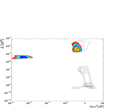
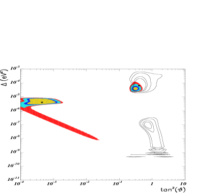
Figure 4: The 90, 95, 99 and 99.73% C.L. contours of the combined fit of solar and SN 1987A data (coloured/grey) together with the contours of the solar data alone (solid lines); for $\tau=\langle E_{\bar{\nu}_{\rm h}}\rangle/\langle E_{\bar{\nu}_{\rm e}}\rangle=1.4$ (top) and $\tau=1.7$ (bottom). All figures for $E_{\rm b}=3\times 10^{53}$ erg and $\langle E_{\bar{\nu}_{\rm e}}\rangle=14$ MeV.

In Fig. 4 we show the C.L. contours of the combined fit for a rather representative set of astrophysical parameters, namely binding energy $E_{\rm b}=3\times 10^{53}$ erg and $\langle E_{\bar{\nu}_{\rm e}}\rangle=14$ MeV. In this case, the impact of the SN 1987A data on the standard solutions to the solar neutrino problem is rather dramatic: the LOW-QVAC and VAC solutions disappear for both assumed $\tau=\langle E_{\bar{\nu}_{\rm h}}\rangle/\langle E_{\bar{\nu}_{\rm e}}\rangle$ values; they are excluded at more than 99.98% even for $\tau=1.4$. Moreover the size of the LMA–MSW solution decreases with increasing $\tau$. The part of the LMA–MSW solution which is most stable against the addition of the supernova data corresponds to the lowest $\Delta$ and $\tan^{2}\vartheta$ values, since these are favoured by Earth matter regeneration effects. On the other hand the SMA–MSW region re-appears extending, for increasing $\tau$, as a funnel towards the VAC solution along the hypotenuse of the solar MSW triangle. The combined best-fit point (star) moves from the LMA–MSW region for $\tau=1.4$ to the SMA–MSW solution for $\tau=1.7$.

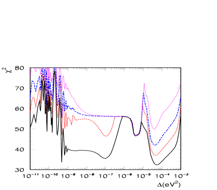
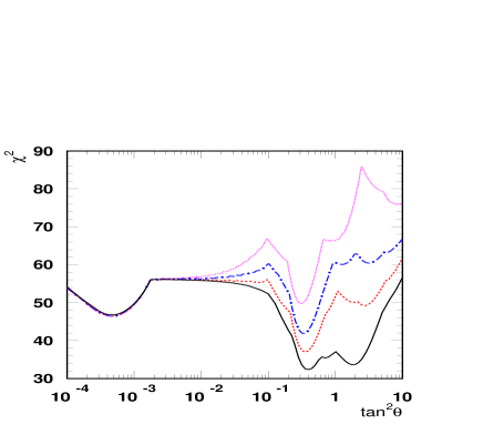
Figure 5: The solid curve indicates the $\chi_{\odot}^{2}$ of the solar neutrino data. The non-solid curves illustrate the effect of adding the SN 1987A data, which worsens the status of large mixing-type solutions; marginalized with respect to $\vartheta$ (top) and to $\Delta$ (bottom), respectively.

In Fig. 5 we illustrate in a global way the relative status of various oscillation after adding the SN 1987A data. For each $\Delta$ value we have optimized the $\chi^{2}$ with respect to $\vartheta$ in the top and with respect to $\Delta$ in the bottom panel. The solid curve indicates $\chi_{\odot}^{2}$, the non-solid curves correspond to the case where the SN 1987A data are included. The dash-dotted line is for $E_{\rm b}=3\times 10^{53}$ erg, $\tau=1.4$ and $\langle E_{\bar{\nu}_{\rm e}}\rangle=14$ MeV. The dashed line is for $E_{\rm b}=3\times 10^{53}$ erg, $\tau=1.4$ and $\langle E_{\bar{\nu}_{\rm e}}\rangle=12$ MeV. The dotted line is for $E_{\rm b}=3\times 10^{53}$ erg, $\tau=1.7$ and $\langle E_{\bar{\nu}_{\rm e}}\rangle=14$ MeV. Here we have adjusted an arbitrary constant which appears when combining the minimum likelihood-type SN 1987A analysis with the solar $\chi^{2}$ data analysis in such a way that the SMA solution gets unaffected by the SN 1987A data. One notices that the effect of adding SN 1987A data is always to worsen the status of the large-mixing angle solutions. Within each such curve one can compare the relative goodness of various solutions, however different curves should not be qualitatively compared.

4 Summary and Discussion

We have discussed non-adiabatic neutrino oscillations in general power-law potentials $A\propto x^{n}$. We found that the resonance point coincides only for a linear profile with the point of maximal violation of adiabaticity. We presented the correct boundary between the adiabatic and non-adiabatic regime for all $\vartheta$ and $n$ as well as a new method to calculate the crossing probability also in the non-resonant regime.

Performing a combined likelihood analysis of the observed neutrino signal of SN 1987A and solar neutrino data including the SNO CC measurement, we found that the supernova data offer additional discrimination power between the different solutions of the solar neutrino puzzle. Unless all relevant supernova parameters lie close to their extreme values found in simulations, the status of the LMA solutions deteriorates, although the LMA–MSW solution may still survive as the best combined fit for acceptable choices of astrophysical parameters. In particular, SN 1987A data generally favour its part with smaller values of $\vartheta$ and $\Delta$. In contrast the vacuum or “just-so” solution is excluded and the LOW solution is significantly disfavoured for most reasonable choices of astrophysics parameters. The SMA–MSW solution is absent at about the $3\sigma$-level if solar data only are included but may reappear once SN 1987A data are added, due to the worsening of the LMA type solutions.

Finally, one should not forget that in the solar case, a well-tested standard solar model exists whose errors are accounted for in the fit. In contrast there is no “standard model” for type II supernovae and therefore also no well-established average values and error estimates for the relevant astrophysical parameters.

References

- [1] A. Friedland, Phys. Rev. D 64 (2001) 013008.
- [2] T.K. Kuo and J. Pantaleone, Phys. Rev. D 39 (1989) 1930.
- [3] M. Kachelrieß and R. Tomàs, Phys. Rev. D 64 (2001) 073002.
- [4] M. Kachelrieß, A. Strumia, R. Tomàs and J.W.F. Valle, hep-ph/0108100.
- [5] We used the data set corresponding to Fig. 6b of P. Creminelli, G. Signorelli and A. Strumia, hep-ph/0102234v2.
- [6] M. Kachelrieß, R. Tomàs and J.W.F. Valle, J. High Energy Phys. 01 (2001) 030.