Phase space veto method for next-to-leading order event generators in hadronic collisions

Abstract

A method for organizing next-to-leading order QCD calculations using a veto which enforces the cancellations between virtual and real emission diagrams is applied to hadronic collisions. The method employs phase space slicing with the slicing parameter determined dynamically event-by-event. It allows for the generation of unweighted events and can be consistently merged with a parton shower. The end product is more intuitive for the end user, as it is probabilistic, and can be easily interfaced to general purpose showering and hadronization programs to obtain a complete event description suitable for experimental analyses. As an example an event generator for the process $pp\!\!\!\!^{{}^{(-)}}\rightarrow Z+X$ at NLO is presented and interfaced consistently to the PYTHIA shower and hadronization package.

24.10.Lx, 12.38.-t, 14.70.-e

Keywords: Monte Carlo simulations, Quantum Chromodynamics, Gauge bosons, Parton shower

I INTRODUCTION

Computer simulations of higher order quantum chromodynamics (QCD) corrections in high energy physics collisions typically rely on one of two methods: the parton shower [1, 2] or numerical integration of next-to-leading order (NLO) distributions. Both methods have proven extremely useful, but each has a limited—though complementary—region of applicability.

Programs which employ the parton shower approach, such as PYTHIA [3], HERWIG [4], and ISAJET [5], have enjoyed widespread use by experimentalists. These programs begin with a leading order hard subprocess. Higher order effects are added by evolving the event using the parton shower, which provides an all orders description of parton emissions valid in the soft and collinear regions, but is not accurate for well-separated particles. The partons are then grouped together into colorless hadrons, resonances are decayed, and the underlying structure of the event (beam remnants, multiple interactions, etc.) is added. These programs are able to describe the exclusive structure of the event, and so provide a useful input for subsequent detector simulation.

NLO integration programs go one order beyond in the prediction of the cross section, have a reduced dependence on arbitrary scale choices, and provide a good description of hard well-separated emissions. They are able to predict distributions of events, but are unable to produce events with the frequency predicted by the theory (because the cancellations between Feynman diagrams are usually achieved by allowing a fraction of phase space points to have negative probability). These programs are commonly used by experimental collaborations for determining $k$-factors, which are often assumed to be constant, and are employed to correct the normalization of distributions from leading order event generators. Lacking individual events to evolve further, it is difficult to add subsequent event features like hadronization or the underlying event. This has meant that these programs are excellent theoretical tools for predictions of distributions, but limits their usefulness for producing events to be simulated in the detector environment. The primary aim of the method presented in this paper is to improve the usefulness of NLO calculations for experimental applications by interpreting the result in a manner which is well suited for interface to showering and hadronization generators and subsequent detector simulation.

The pursuit of techniques for combining NLO calculations with the parton shower is a natural direction for the evolution of event generators. Two primary challenges stand in the way: overlaps between phase space volumes of differing dimensionality need to be accounted for in a manner which does not double-count or neglect any region, and the result needs to be interpretable in a probabilistic way (probabilities should be everywhere positive definite). Significant advances towards the resolution of the former challenge have been achieved by Collins [6] using a subtractive approach, however negative weighted events are still produced.

The issue of unweighted event generation has been addressed by the author for the special case of diboson production in Ref. [7], then further developed to include a consistent merging of the parton shower in Ref. [8]. In the present study, these techniques are generalized and a veto method proposed by Pötter [9] is incorporated. This allows for the organization of NLO event generators in an elegant and simple manner which competes with leading order event generators in terms of efficiency and computer time.

To illustrate the methods discussed in this paper, an event generator for the process $pp\!\!\!\!^{{}^{(-)}}\rightarrow l^{+}l^{-}+X$ is constructed and used to generate event distributions relevant to the Fermilab Tevatron Collider and the CERN Large Hadron Collider (LHC). A precise knowledge of the Drell-Yan lepton pair production process is particularly important at hadron colliders. It will be used to probe new physics (e.g. large extra dimensions, extra neutral gauge bosons), perform precision measurements of electroweak parameters, constrain the parton density functions, and calibrate the detector. The latter is perhaps most important to the physics program, because it means our knowledge of this process will feed into the systematic errors for most physics measurements: the lepton energy and momentum scale may be calibrated in situ with $Z^{0}\rightarrow l^{+}l^{-}$ events, the jet energy scale may be determined using events with a $Z^{0}$ decaying to leptons recoiling against a high transverse momentum jet, and the Drell-Yan event rate may be used to determine the absolute luminosity. The NLO QCD corrections to the process have been available for some time [10]. Recently the complete ${\cal O}$($\alpha_{\mathrm{QED}}$) corrections have been calculated [11], and will play an important role for precision measurements.

In the following section, background information relevant to the NLO calculation is presented. A description of the phase space veto method, numerical results, and shower evolution are presented in the next sections.

II BACKGROUND

The NLO cross section receives contributions from the square of the Born graphs, the interference of the Born graphs with the one-loop graphs, and the square of the real emission graphs which contain an extra colored parton in the final state,

$${\cal{M}}^{2}_{\mathrm{NLO}}~{}=~{}{\cal{M}}^{2}_{\mathrm{Born}}+{\cal{M}}_{\mathrm{Born}}\otimes{\cal{M}}_{\mathrm{one~{}loop}}+{\cal{M}}^{2}_{\mathrm{real~{}emission}}.$$ (1)

The second and third terms of Eq. 1 diverge when treated separately, and so numerical integration calculations employ a regularization scheme which effectively combines pieces of these terms to obtain finite results everywhere in phase space.

Commonly used schemes include the “subtraction method” [12], “dipole method” [13], and “phase space slicing” (PSS) methods [14, 15, 16, 17, 18]. All methods give identical results when used appropriately. For the purposes of this study, features of the PSS methods are convenient. Variations of the PSS method include the “two parameter PSS” [14] (see Ref. [15] for an accessible review), “one parameter PSS” [16], and “$\mathrm{s}_{\mathrm{min}}$-slicing” [17, 18].

To illustrate the PSS method, consider $pp\!\!\!\!^{{}^{(-)}}\rightarrow Z^{0}+X$ at NLO. The Feynman graphs are presented in Figure 1. The first term of Eq. 1 is leading order ($\alpha_{\mathrm{QED}}$) and contains $n$ particles in the final state. The phase space volume $\Phi_{\mathrm{n}}$ which defines the configuration of the four-vectors is referred to as n-body and specified by 4 degrees of freedom: the $Z^{0}$ mass, $Z^{0}$ boost, and two $Z^{0}$ decay angles. The second term of Eq. 1 is first order ($\alpha_{\mathrm{QED}}$$\alpha_{\mathrm{S}}$) and is also described by n-body kinematics. The third term of Eq. 1 is also first order ($\alpha_{\mathrm{QED}}$$\alpha_{\mathrm{S}}$) and the final state contains the vector-boson (or its decay products) and a colored parton (e.g. $Z^{0}g,~{}Z^{0}q,~{}Z^{0}\bar{q}$) and is described by (n+1)-body kinematics with 7 degrees of freedom: the system mass, system boost, $Z^{0}$ mass, two $Z^{0}$ production angles, and two $Z^{0}$ decay angles.

For a particular choice of the n-body kinematics, the phase space $\Phi_{+1}$ which specifies the kinematics of the real emission is a plane in $\hat{u}=(p_{2}-p_{j})^{2}$ vs. $\hat{t}=(p_{1}-p_{j})^{2}$ space, shown in Figure 2, where $p_{1}$ and $p_{2}$ are the four-momenta of the massless colliding partons, and $p_{j}$ is the massless colored emission (the azimuthal degree of freedom is unimportant and not shown). The n-body kinematics occupy a point at the origin of this plane. The corresponding differential cross section diverges as either axis of the plane is approached and at the origin, i.e. when the emission becomes soft or collinear.

The PSS methods regulate the singularities by partitioning the phase space into a region of resolved emissions, and a region of unresolved soft and collinear emissions. The resolved part is integrated numerically. The contribution from the unresolved soft and collinear emissions is calculated analytically and included with the n-body squared matrix element such that the net result is finite, though not necessarily positive. For the case of $\mathrm{s}_{\mathrm{min}}$-slicing, the boundary of the unresolved region is defined by a single parameter with dimension energy squared. An emission is considered to be unresolved anytime the invariant mass squared of any parton pair is less than the $\mathrm{s}_{\mathrm{min}}$ resolution parameter

$$|s_{ij}|~{}<~{}\mathrm{s}_{\mathrm{min}}\hskip 42.67912pt\mbox{(unresolved region)}$$ (2)

where the partons $i,~{}j$ may be either initial or final state.

The cross section for a particular n-body configuration $\Phi_{\mathrm{n}}$, integrated over the entire $\hat{u}$ vs. $\hat{t}$ plane of Figure 2 is a constant, schematically

$$\sigma^{\mathrm{n}}(\Phi_{\mathrm{n}},\mathrm{s}_{\mathrm{min}})~{}+~{}\int_{s_{ij}>\mathrm{s}_{\mathrm{min}}}\sigma^{\mathrm{n+1}}(\Phi_{\mathrm{n}},\Phi_{+1})d\Phi_{+1}~{}=~{}\mbox{\sc Const}(\Phi_{\mathrm{n}})$$ (3)

and is independent of the $\mathrm{s}_{\mathrm{min}}$ choice. For a complete description of $\mathrm{s}_{\mathrm{min}}$-slicing refer to [17, 18].

There exists a boundary in the unresolved region of $\hat{t}$ vs. $\hat{u}$ space, referred to here as $\mathrm{s}_{\mathrm{zero}}$, inside which the sum of the n-body and (n+1)-body contributions is zero. Knowing the location of the boundary, one could calculate the NLO cross section and distributions by sampling only the (n+1)-body phase space, restricted to that region which lies above the boundary (resolved partons). Thus $\sigma^{\mathrm{n}}(\Phi_{\mathrm{n}},\mathrm{s}_{\mathrm{zero}})=0$ and the constant of Eq. 3 is

$$\int_{s_{ij}>\mathrm{s}_{\mathrm{zero}}}\sigma^{\mathrm{n+1}}(\Phi_{\mathrm{n}},\Phi_{+1})d\Phi_{+1}~{}=~{}\mbox{\sc Const}(\Phi_{\mathrm{n}}).$$ (4)

The analytic expression for $\sigma^{\mathrm{n}}(\Phi_{\mathrm{n}},\mathrm{s}_{\mathrm{min}})$ is given in Ref. [18], and the analytic expression for $\mathrm{s}_{\mathrm{zero}}$ is derived in the appendix of the present paper.

A variant of the idea was originally proposed by Baer and Reno in Ref. [19], who approximated the $\mathrm{s}_{\mathrm{zero}}$ boundary as constant and evaluated it by trial and error for single vector-boson production in hadronic collisions using the two parameter PSS method. However, the location of the boundary varies event-by-event with the n-body kinematics. This was demonstrated by Pötter [9], who formulated techniques for evaluating the $\mathrm{s}_{\mathrm{zero}}$ boundary dynamically event-by-event. The idea has been implemented for jet production in deep inelastic scattering in Ref. [20], and good agreement is found with the Hera data.

III THE PHASE SPACE VETO METHOD

To illustrate the phase space veto ($\Phi$-space Veto) method for hadronic collisions, the process $pp\!\!\!\!^{{}^{(-)}}\rightarrow Z^{0}+X\rightarrow l^{+}l^{-}+X$ is chosen. As for the PSS methods, the phase space is divided into two distinct volumes. The n-body volume encompasses the phase space with no resolved emission ($pp\!\!\!\!^{{}^{(-)}}\rightarrow Z^{0}\rightarrow l^{+}l^{-}$ kinematics), while the (n+1)-body volume describes the phase space with an extra parton in the final state, $pp\!\!\!\!^{{}^{(-)}}\rightarrow Z^{0}j\rightarrow l^{+}l^{-}j$, where $j$ denotes a gluon or (anti)quark. For the PSS method, the two volumes would be integrated separately using numerical techniques, and then added together.

For the $\Phi$-space Veto method, the integration is organized differently. Only the (n+1)-body volume is integrated, and the n-body matrix elements are used to test on which side of the $\mathrm{s}_{\mathrm{zero}}$ boundary each phase space point lies. An event candidate sampled in the (unrestricted) (n+1)-body phase space represents a point in the $\hat{u}$ vs. $\hat{t}$ plane shown in Figure 2. If the point lies below the $\mathrm{s}_{\mathrm{zero}}$ boundary, the event is veto-ed. If it lies above the boundary, it is assigned the event weight from the (n+1)-body differential cross section. Since the location of the $\mathrm{s}_{\mathrm{zero}}$ boundary depends on both the factorization and renormalization scales, the reduced scale dependence of the NLO calculation is maintained.

There are at least two possibilities for determining on which side of the boundary a phase space point lies:

1. the location of the $\mathrm{s}_{\mathrm{zero}}$ boundary can be calculated analytically. The n-body cross section is a quadratic equation in $\ln\mathrm{s}_{\mathrm{min}}$, with the smaller of the two roots corresponding to the correct solution. This is the method proposed in Refs. [9, 20], where the $\mathrm{s}_{\mathrm{zero}}$ equations for single jet production in electron-proton scattering are derived. In the appendix of the present paper, the corresponding $\mathrm{s}_{\mathrm{zero}}$ equations for $pp\!\!\!\!^{{}^{(-)}}\rightarrow Z^{0}/\gamma^{\star}$ at NLO are derived.

2. without knowing the location of the $\mathrm{s}_{\mathrm{zero}}$ boundary in the unresolved region explicitly, it is possible to test on which side of the boundary a phase space point lies by projecting the (n+1)-body kinematics onto n-body kinematics and simply evaluating the sign of the n-body matrix element with the $\mathrm{s}_{\mathrm{min}}$ boundary adjusted to sit on top of the point in the $\hat{u}$ vs. $\hat{t}$ plane. It is not necessary to keep track of Jacobians from the projection nor overall normalization factors, since only the sign of the matrix element is of interest. One must be careful because well above the $\mathrm{s}_{\mathrm{zero}}$ boundary (and after the $\mathrm{s}_{\mathrm{min}}$-slicing approximation has broken down) the n-body cross section turns negative once again (corresponding to the second solution of the quadratic equation in $\ln\mathrm{s}_{\mathrm{min}}$, discussed above). In practice this happens only at large ($\approx 10^{5}{\mathrm{G}eV}^{2}$) values of $\mathrm{s}_{\mathrm{min}}\gg 100{\mathrm{G}eV}^{2}$ (see Figure 3). This strategy is simple to implement, and works for $\mathrm{s}_{\mathrm{min}}$-slicing, one parameter PSS, and two parameter PSS. In this manner, processes which have already been coded as a numerical integration using one of the PSS methods can be re-cast as event generators with minimal effort.

Regardless of which of the above techniques is chosen, it is necessary to project 7 dimension (n+1)-body kinematics onto the 4 dimension n-body ones. This is accomplished by requiring the lepton-pair mass $M_{\mathrm{l^{+}l^{-}}}$, and rapidity $Y_{l^{+}l^{-}}$, to remain unchanged in the projection. To perform the projection, the center of mass frame lepton momenta are boosted into the vector-boson rest frame (which is the ‘new center of mass frame’), and then boosted longitudinally such that the pair regains their original rapidity, $Y_{l^{+}l^{-}}$.

In Figure 4 the $\mathrm{s}_{\mathrm{zero}}$ boundary for the Tevatron and LHC collider energies are shown as a function of the lepton-pair rapidity for several parton center of mass choices. The dependence of the $\mathrm{s}_{\mathrm{zero}}$ boundary on the choice of renormalization and factorization scales is shown in Figure 5.

Though the $\mathrm{s}_{\mathrm{zero}}$ boundary always exists, there is no guarantee that the boundary lies within the region of validity for the PSS methods. This has not been a problem for the limited set of processes to which the method has been applied. However, a hybrid of the PSS and subtraction methods [21] has been proposed in Ref. [9] to deal with the situation, should the need arise.

For each phase space sample in the above algorithm, both the (n+1)-body and n-body matrix elements are evaluated. This means that the event generation will be slower than that for tree level events by the amount of computer time it takes to evaluate the n-body matrix elements which are used to perform the veto. Though this appears to be the minimal computation necessary for performing a calculation which incorporates the full NLO information, this is not the case. There are ways in which the performance, in terms of computational time, can be improved:

• upper and lower limits on $\mathrm{s}_{\mathrm{zero}}$ can be evaluated (see Figure 4). For phase space points which lie outside of these limits, the n-body matrix element need not be evaluated to determine whether or not the point is veto-ed. For Tevatron energy, $\mathrm{s}_{\mathrm{zero}}$ ranges from about 1 GeV² to about 100 GeV².

• since event generation is normally implemented using the hit-and-miss (i.e. acceptance/rejection) Monte Carlo technique, the majority of event candidates will be rejected anyway. The $\Phi$-space Veto need be applied only to those event candidates which are accepted (or whenever an event candidate violates the maximum event weight against which the acceptance/rejection is taking place). Since the efficiency of event generators is typically about 25% or lower, it means that the n-body matrix element needs to be evaluated rarely. Further, when the event candidates are sampled from an adaptive integration grid (such as for the implementation presented in this paper), the adaptive integration will “learn” the location of the boundary, and will bias the sampling away from the region below the boundary.

IV NUMERICAL RESULTS

The $pp\!\!\!\!^{{}^{(-)}}\rightarrow Z^{0}+X\rightarrow l^{+}l^{-}+X$ event generator is implemented using the squared matrix elements of Ref. [22] cast into the $\mathrm{s}_{\mathrm{min}}$-slicing method [18] (which employs special ‘crossed’ structure functions). The matrix elements include both the $Z^{0}$ and $\gamma^{\star}$ diagrams with decay to massless leptons, such that the branching ratio to one lepton flavor is automatically included. This means finite width effects, lepton decay correlations, and forward-backward asymmetries are everywhere taken into account. The generator is written in C++ using modern object-oriented design patterns. A new prototype C++ version of the Bases/Spring program [23] is used for adaptive integration and event generation. Special care has been taken to make the program user friendly, and it is available upon request from the author.

All of the distributions and cross sections presented in this paper are for $p\bar{p}$ collisions at 2 TeV (Tevatron Run II) or $pp$ collisions at 14 TeV (LHC), with the lepton-pair mass restricted  to the range 66-116 GeV and decaying to $e^{-}e^{+}$. CTEQ3M [24] parton density functions are used (chosen because the ‘crossed’ versions of the structure functions [18] are readily available, though in principle they can be tabulated for any structure function). For all calculations the renormalization and factorization scales have been set equal to the vector-boson mass, $\mu_{R}=\mu_{F}=M_{\mathrm{l^{+}l^{-}}}$, and the $\overline{\mathrm{MS}}$ factorization scheme is used. The input parameters are chosen to coincide with those in PYTHIA 6.200: the $Z^{0}$ mass and width are $M_{Z}=91.188$ GeV and $\Gamma_{Z}=2.47813$ GeV, the electroweak mixing angle is $\sin^{2}\theta_{W}=0.232$, and the electroweak coupling is $\alpha_{\mathrm{QED}}$$(M_{Z})=1/128.8$. The two-loop $\overline{\mathrm{MS}}$ expression for $\alpha_{\mathrm{S}}$ is used with $\Lambda^{4,\overline{\mathrm{MS}}}=0.239$ GeV. Using these input parameters, the $\Phi$-space Veto event generator predicts $239.7\pm 0.6$ pb for the inclusive cross section at Tevatron Run II.

In Figure 6 the inclusive cross section prediction from the $\Phi$-space Veto event generator is compared to the predictions from the $\mathrm{s}_{\mathrm{min}}$-slicing calculation using several choices of the $\mathrm{s}_{\mathrm{min}}$ parameter. The results are consistent, indicating the $\mathrm{s}_{\mathrm{zero}}$ boundary lies within the region where the $\mathrm{s}_{\mathrm{min}}$-slicing approximation is valid.

In Figure 7 distributions produced with the $\Phi$-space Veto event generator are compared to those derived from numerical integrations using $\mathrm{s}_{\mathrm{min}}$-slicing. The $\Phi$-space Veto method faithfully reproduces the NLO transverse momentum of the electron. The transverse momentum of the vector-boson also agrees well with the $\mathrm{s}_{\mathrm{min}}$-slicing everywhere that the NLO calculation is valid.

In the small $P^{T}_{\mathrm{Z}}$ region, multiple gluon emission becomes important and fixed order perturbation theory is unreliable. This is evident in the inset of Figure 7. In this region the results depend on the specific choice of the $\mathrm{s}_{\mathrm{min}}$ parameter. This is also the region where the $\Phi$-space Veto method becomes unreliable because the minimum jet scale is coupled to the n-body kinematics. This effect is visible in Figure 8, where the kinematics of the veto-ed event candidates from the $\Phi$-space Veto method for a typical event generation run are plotted in the $P^{T}_{\mathrm{Z}}$ vs. $\mathrm{s}_{\mathrm{min}}$ plane. The largest $P^{T}_{\mathrm{Z}}$ of a veto-ed candidate event is 5.5 GeV, indicating the NLO calculation is unable to provide a useful prediction in the region below $\approx 5.5$ GeV. It is worth stressing that this does not make the $\Phi$-space Veto method less useful than $\mathrm{s}_{\mathrm{min}}$-slicing since any NLO calculation is unreliable here. This is the region where the distributions are better modeled with the parton shower, and a suitable treatment which removes this minimum jet scale coupling will be provided in the next section. The $\mathrm{s}_{\mathrm{zero}}$ boundary represents a lower limit to the usefulness of our fixed order perturbative approximation. As such, $\mathrm{s}_{\mathrm{zero}}$ is a useful concept as a qualitative measurement of the frontier of the validity of our perturbative calculation.

In Figure 9 the factorization and renormalization scale dependence of the transverse momentum of the electron and vector-boson distributions are shown using the $\Phi$-space Veto method for Tevatron and LHC energies. The scale dependence is identical to that from the $\mathrm{s}_{\mathrm{min}}$-slicing method, because the $\mathrm{s}_{\mathrm{zero}}$ boundary encodes information about the scale choices (Figure 5). The change in the distributions resulting from the variation of the scales is an indication of the theoretical error arising from neglected higher order terms. The importance of the reduced scale dependence is demonstrated in Figure 10, where the variation in the prediction at Born level and at NLO of the transverse momentum of the electron for $pp\rightarrow Z^{0}+X\rightarrow e^{+}e^{-}+X$ at LHC energy is shown. The comparison is restricted to that region where the Born level prediction is meaningful. The same comparison is shown for the lepton-pair mass distribution in Figure 11. The change in the scale at Born level results in more than a 25% variation in the distributions, whereas the prediction from the NLO $\Phi$-space Veto generator reduces this variation to about 7%. The scale dependence arising in predictions from event generators which use leading order subprocesses (like PYTHIA, HERWIG, and ISAJET) will resemble that of the Born level prediction.

V SHOWER EVOLUTION

At the present stage, each event consists of the vector-boson decay products and exactly one colored emission in the final state. The energy scale of the emission is at least $\sqrt{\mathrm{s}_{\mathrm{zero}}}$. Unweighted events are provided by the Bases/Spring algorithm, and the normalization is NLO. A coupling between the minimum emission scale $\sqrt{\mathrm{s}_{\mathrm{zero}}}$ and the kinematic configuration exists in the very small $P^{T}_{\mathrm{Z}}$ region.

The next step is a consistent interface to a parton shower algorithm. The goal is to have the parton shower dominate the prediction in the soft/collinear region (in particular, it should preserve the parton shower’s prediction of Sudakov suppression [25]), and the first order tree level diagrams dominate in the region of hard well separated partons. This does not compromise the integrity of the prediction, it merely highlights that different approaches are well-suited to different regions.

To accomplish this, a parameter $\mathrm{s}_{\mathrm{P.S.}}$ is introduced to partition a region of $\hat{t}$ vs. $\hat{u}$ space which is exclusively the domain of the parton shower. This parameter may be thought of as separating the fixed order regime from the all-orders parton shower region, in the same way that a ${\cal O}$(1 GeV) parameter in the showering and hadronization programs defines the scale at which the parton shower is terminated, and the simulation turns to the non-perturbative hadronization model for a description of the physics. This partition is shown in Figure 12. Events which lie below the $\mathrm{s}_{\mathrm{P.S.}}$ boundary are first projected onto n-body kinematics (i.e. the point in $\hat{t}$ vs. $\hat{u}$ space is moved to the origin) and the parton shower is allowed to evolve the event out into the plane. The projection is performed keeping the lepton-pair mass and rapidity fixed, exactly as described in Sec. III. The parton shower is invoked with the scale set to $\sqrt{\mathrm{s}_{\mathrm{P.S.}}}$, which ensures the evolution does not move the event out into a region of phase space which has already been counted using the first order tree level matrix elements.

A reasonable choice for the $\sqrt{\mathrm{s}_{\mathrm{P.S.}}}$ parameter is a few times the minimum jet scale, $\sqrt{\mathrm{s}_{\mathrm{zero}}}$. This ensures the first order tree level matrix element is reliable above the $\mathrm{s}_{\mathrm{P.S.}}$ boundary. The distributions have very little sensitivity to the choice of $\mathrm{s}_{\mathrm{P.S.}}$.

For events which lie above the $\mathrm{s}_{\mathrm{P.S.}}$ region, the parton shower is also invoked, this time with a scale equal to the minimum invariant mass of any parton-pair

$$\mbox{parton~{}shower~{}scale}~{}=~{}\mbox{minimum}\left[~{}Q_{q\bar{q}},~{}Q_{qg},~{}Q_{\bar{q}g}~{}\right]$$ (5)

which ensures no double counting can occur.

The effect of the projection and subsequent parton showering is shown in Figure 13. Initially the distributions are provided by the $\Phi$-space Veto, solid line. The projection is applied to events which sit below the $\mathrm{s}_{\mathrm{P.S.}}$ boundary, which effects only the small $P^{T}_{\mathrm{Z}}$ region, and is shown as a dashed line and does not correspond to anything physical. Finally the parton shower is applied (dotted line), and has the largest effect on those events which have been projected.

In Figure 14 the $\Phi$-space Veto event distributions (including parton shower evolution) are shown for several choices of the $\mathrm{s}_{\mathrm{P.S.}}$ parameter. The dependence on the $\mathrm{s}_{\mathrm{P.S.}}$ parameter choice is small, indicating discontinuities which might exist at the $\mathrm{s}_{\mathrm{P.S.}}$ boundary are also small.

For the distributions presented here, events from the $\Phi$-space Veto generator have been evolved with the PYTHIA 6.200 parton shower. PYTHIA is attached using the HepUP interface [26], which is a generic standard for the communication between event generators. Having evolved the events through the parton shower, PYTHIA provides other features of the event structure such as hadronization, resonance decays, beam remnants, and multiple interactions. The showered event distributions presented in this paper include all of these features. The use of the HepUP interface allows for the parton shower program to be easily interchanged. The choice of PYTHIA is arbitrary, there is nothing which precludes the use of any other showering program.

The full event generator is now complete. Adaptive integration and phase space generation is provided by BasesSpring. The event weights are evaluated using the $\Phi$-space Veto method, which discards those event candidates lying below the $\mathrm{s}_{\mathrm{zero}}$ boundary. When the program is executed, the phase space is first mapped onto a grid using an initialization pass with the adaptive integration (performed by the ‘Bases’ part of the BasesSpring package). The ‘Spring’ part of the BasesSpring package then provides unweighted events, by sampling candidate events from the adaptive integration grids and accepting events according to the differential cross section using the acceptance-rejection algorithm. After removing the emission from those events which are soft or collinear (as defined by the $\mathrm{s}_{\mathrm{P.S.}}$ parameter), the events are transferred to the PYTHIA package using the HepUP interface. PYTHIA performs the parton shower, and subsequent event evolution including hadronization, etc.

While the end result in terms of physics does not differ significantly from that obtained by the author in Ref. [8] for $WZ$ production, the method presented here is simpler, easier to implement, faster in terms of computer time, and may be generalized to a broad range of processes. Improved methods for invoking the parton shower from parton level event configurations are being developed [28, 29], and are suitable for application to the $\Phi$-space Veto events.

A comparison of the computer time for generating the events is presented in Table I. The processing time per event and generation efficiency (percentage of candidate weighted events which are accepted in the event generation algorithm) for PYTHIA and the $\Phi$-space Veto are similar, indicating the $\Phi$-space Veto method is successful in encoding the extra NLO information without affecting the overall time-performance of event generation.

In Figure 15 the $\Phi$-space Veto distributions (solid line, includes evolution with the PYTHIA showering and hadronization package) are compared to the predictions from PYTHIA. In PYTHIA there are two strategies implemented for single vector-boson production. For both strategies the hard subprocess is chosen according to the Born level matrix element, such that the normalization is always leading order. For the “old” PYTHIA implementation of the process, the event is then evolved with the standard parton shower beginning at a scale equal to the vector-boson mass. For the new “matrix element (M.E.) corrected” implementation of the process, [31] the shower is initiated at a scale equal to the machine energy and is corrected according to the $Z^{0}$+jet first order tree level matrix element, which results in a considerable improvement of the high $P^{T}_{\mathrm{Z}}$ region modeling. The virtual one-loop contribution is not included anywhere in the PYTHIA implementations. The dotted line in Figure 15 is from the standard PYTHIA process, and the dashed line is from the M.E. PYTHIA process. The $\Phi$-space Veto distribution and M.E. corrected PYTHIA shapes are rather similar, indicating the matrix element corrections in PYTHIA are having the desired effect. The $\Phi$-space Veto distributions have the advantage of NLO normalization and a reduced dependence on the factorization and renormalization scales.

VI CONCLUSIONS

The $\Phi$-space Veto method for organizing NLO calculations into event generators is demonstrated for $Z^{0}$ production in hadronic collisions. The method is based loosely on the ideas proposed by Pötter for deep inelastic scattering [9]. The primary motivation for the method is to move numerical NLO calculations beyond the status of “event integrators” to “event generators”, making them suitable for interface to showering and hadronization programs and subsequent detector simulation.

The general features of the $\Phi$-space Veto method are:

• event weights are positive definite, meaning the standard methods for event generation can be applied, providing a prediction which is well suited for experimental applications.

• in the soft/collinear region, the results are dominated by the parton shower. In particular the low $P^{T}_{\mathrm{}}$ region exhibits Sudakov suppression.

• in the region of hard well separated partons, the distributions are dominated by the first order matrix element.

• the normalization is NLO and the reduced scale dependence afforded by the NLO calculation is maintained.

The method has been implemented as an event generator (available from the author) for $pp\!\!\!\!^{{}^{(-)}}\rightarrow Z^{0}/\gamma^{\star}+X\rightarrow l^{+}l^{-}+X$, with showering and hadronization provided by the PYTHIA package.

APPENDIX: The $\mathrm{s}_{\mathrm{zero}}$ Function for $pp\!\!\!\!^{{}^{(-)}}\rightarrow Z^{0}+X$ at NLO

The differential cross section for the n-body contribution to $pp\!\!\!\!^{{}^{(-)}}\rightarrow Z^{0}+X$ evaluated in the $\overline{\mathrm{MS}}$ scheme, integrated over unresolved emissions out to a scale of $\mathrm{s}_{\mathrm{min}}$, and neglecting overall factors, is a quadratic equation in $\ln\mathrm{s}_{\mathrm{min}}$

(6)

$\displaystyle d\sigma^{\mathrm{NLO}}_{\mathrm{n-body}}~{}\propto~{}\sum_{ij}\left\{\hskip 14.22636pt\left[1~{}+~{}\frac{\mbox{$\alpha_{\mathrm{S}}$}(\mu_{R})}{2\pi}\frac{N_{C}^{2}-1}{N_{C}}\left(-(\ln\frac{\mathrm{s}_{\mathrm{min}}}{\hat{s}})^{2}+\frac{\pi^{2}}{2}\cdot\frac{1}{3}-2\cdot\frac{3}{4}\ln\frac{\mathrm{s}_{\mathrm{min}}}{\hat{s}}-\frac{9}{18}\right)\right]\right.$

$\displaystyle\mbox{}\hskip 142.26378pt\times~{}|{\cal{M}}^{ij}_{\mathrm{Born}}|^{2}f_{P_{1}\rightarrow i}(x_{1},\mu_{F})f_{P_{2}\rightarrow j}(x_{2},\mu_{F})$

$\displaystyle\mbox{}\hskip 92.47145pt~{}+~{}\frac{\mbox{$\alpha_{\mathrm{S}}$}(\mu_{R})}{2\pi}N_{C}|{\cal{M}}^{ij}_{\mathrm{Born}}|^{2}~{}\left[~{}f_{P_{1}\rightarrow i}(x_{1},\mu_{F})\left(A_{P_{2}\rightarrow j}(x_{2},\mu_{F})\ln\frac{\mathrm{s}_{\mathrm{min}}}{\mu_{F}^{2}}~{}+~{}B^{\overline{\mathrm{MS}}}_{P_{2}\rightarrow j}(x_{2},\mu_{F})\right)\right.$

$\displaystyle\mbox{}\hskip 184.9429pt~{}+~{}\left.\left.\left(A_{P_{1}\rightarrow i}(x_{1},\mu_{F})\ln\frac{\mathrm{s}_{\mathrm{min}}}{\mu_{F}^{2}}~{}+~{}B^{\overline{\mathrm{MS}}}_{P_{1}\rightarrow i}(x_{1},\mu_{F})\right)f_{P_{2}\rightarrow j}(x_{2},\mu_{F})~{}\right]~{}\right\},$

where the sum runs over all flavors of initial state (anti)quarks, $N_{C}=3$ is the number of quark colors, $\sqrt{\hat{s}}$ is the vector-boson mass, ${\cal{M}}^{ij}_{\mathrm{Born}}$ is the Born level matrix element for ${q\!\!\!\!^{{}^{(-)}}}_{i}{q\!\!\!\!^{{}^{(-)}}}_{j}\rightarrow Z^{0}$, $f_{P\rightarrow q\!\!\!\!^{{}^{(-)}}}(x,\mu_{F})$ is the parton density function evaluated at Bjorken momentum fraction $x$ and factorization scale $\mu_{F}$, the renormalization scale is $\mu_{R}$ (often $\mu_{F}=\mu_{R}=\sqrt{\hat{s}}$ is chosen), and

$$A_{P\rightarrow q\!\!\!\!^{{}^{(-)}}}(x,\mu_{F})\ln\frac{\mathrm{s}_{\mathrm{min}}}{\mu_{F}^{2}}~{}+~{}B^{\overline{\mathrm{MS}}}_{P\rightarrow q\!\!\!\!^{{}^{(-)}}}(x,\mu_{F})$$ (7)

are the crossed structure functions presented in Eq. 3.37 of Ref. [18].

The solution for $\mathrm{s}_{\mathrm{zero}}$ corresponds to the smaller of the two roots of Eq. 6

$$\mathrm{s}_{\mathrm{zero}}~{}=~{}\mbox{minimum}\left[~{}\hat{s}\times\exp\left(\frac{-b-\sqrt{b^{2}-4ac}}{2a}\right),~{}\hat{s}\times\exp\left(\frac{-b+\sqrt{b^{2}-4ac}}{2a}\right)~{}\right]$$ (8)

with

$$\begin{array}[]{lll}a~{}={}&\sum_{ij}&-\frac{\mbox{$\alpha_{\mathrm{S}}$}(\mu_{R})}{2\pi}\frac{N_{C}^{2}-1}{N_{C}}|{\cal{M}}^{ij}_{\mathrm{Born}}|^{2}f_{P_{1}\rightarrow i}(x_{1},\mu_{F})f_{P_{2}\rightarrow j}(x_{2},\mu_{F})\\ \\ b~{}={}&\sum_{ij}&-2\cdot\frac{3}{4}\frac{\mbox{$\alpha_{\mathrm{S}}$}(\mu_{R})}{2\pi}\frac{N_{C}^{2}-1}{N_{C}}|{\cal{M}}^{ij}_{\mathrm{Born}}|^{2}f_{P_{1}\rightarrow i}(x_{1},\mu_{F})f_{P_{2}\rightarrow j}(x_{2},\mu_{F})\\ \\ &&+~{}\frac{\mbox{$\alpha_{\mathrm{S}}$}(\mu_{R})}{2\pi}N_{C}|{\cal{M}}^{ij}_{\mathrm{Born}}|^{2}~{}\left[f_{P_{1}\rightarrow i}(x_{1},\mu_{F})A_{P_{2}\rightarrow j}(x_{2},\mu_{F})~{}+~{}A_{P_{1}\rightarrow i}(x_{1},\mu_{F})f_{P_{2}\rightarrow j}(x_{2},\mu_{F})\right]\\ \\ c~{}={}&\sum_{ij}&\hskip 14.22636pt\left[1~{}+~{}\frac{\mbox{$\alpha_{\mathrm{S}}$}(\mu_{R})}{2\pi}\frac{N_{C}^{2}-1}{N_{C}}\left(+\frac{\pi^{2}}{2}\cdot\frac{1}{3}-\frac{9}{18}\right)\right]|{\cal{M}}^{ij}_{\mathrm{Born}}|^{2}f_{P_{1}\rightarrow i}(x_{1},\mu_{F})f_{P_{2}\rightarrow j}(x_{2},\mu_{F})\\ \\ &&+~{}\frac{\mbox{$\alpha_{\mathrm{S}}$}(\mu_{R})}{2\pi}N_{C}|{\cal{M}}^{ij}_{\mathrm{Born}}|^{2}~{}\left[f_{P_{1}\rightarrow i}(x_{1},\mu_{F})\left(A_{P_{2}\rightarrow j}(x_{2},\mu_{F})\ln\frac{\hat{s}}{\mu_{F}^{2}}~{}+~{}B^{\overline{\mathrm{MS}}}_{P_{2}\rightarrow j}(x_{2},\mu_{F})\right)\right.\\ \\ &&\mbox{}\hskip 85.35826pt~{}+~{}\left.\left(A_{P_{1}\rightarrow i}(x_{1},\mu_{F})\ln\frac{\hat{s}}{\mu_{F}^{2}}~{}+~{}B^{\overline{\mathrm{MS}}}_{P_{1}\rightarrow i}(x_{1},\mu_{F})\right)f_{P_{2}\rightarrow j}(x_{2},\mu_{F})\right]\end{array}$$ (9)

      Born                              one-loop

                               real emission

FIG. 1.: Feynman graphs contributing to $pp\!\!\!\!^{{}^{(-)}}\rightarrow Z^{0}+X$ at NLO. The wavy line represents either a $Z^{0}$ or $\gamma^{\star}$, and the vector-boson decay products are not shown.

FIG. 2.: A projection of the $pp\!\!\!\!^{{}^{(-)}}\rightarrow Z^{0}j$ phase space onto the $\hat{u}$ vs. $\hat{t}$ plane is shown, where $\hat{u}=(p_{2}-p_{j})^{2}=-Q^{2}_{2j}$ and $\hat{t}=(p_{1}-p_{j})^{2}=-Q^{2}_{1j}$, and $p_{1},~{}p_{2},~{}p_{j}$ are the momenta of the forward colliding parton, backward colliding parton, and real emission. The area above (below) the $\mathrm{s}_{\mathrm{min}}$ boundary is the region of resolved (unresolved) real emissions. When $\mathrm{s}_{\mathrm{min}}=\mathrm{s}_{\mathrm{zero}}$, it denotes the boundary defining the region inside of which the the n-body and (n+1)-body contributions sum to zero (i.e. the cross section integrated over the unresolved region is zero).

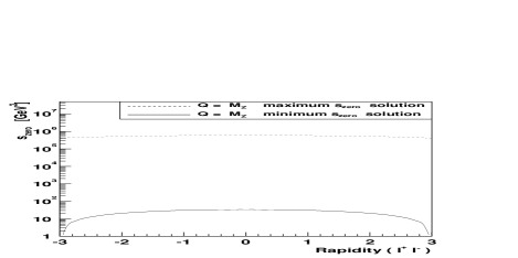
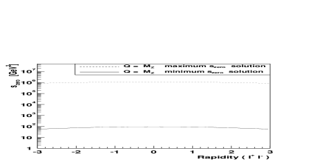
FIG. 3.: The two roots of the quadratic n-body differential cross section presented in Eq. 6 are plotted as a function of the lepton-pair rapidity, evaluated at parton center-of-mass energy equal to the $Z^{0}$ mass for $p\bar{p}$ collisions at 2 TeV (Tevatron, top) and for $pp$ collisions at 14 TeV (LHC, bottom). The smaller solution is the $\mathrm{s}_{\mathrm{zero}}$ function of interest, the larger solution should not be interpreted physically.

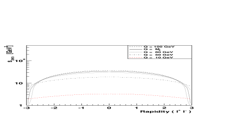
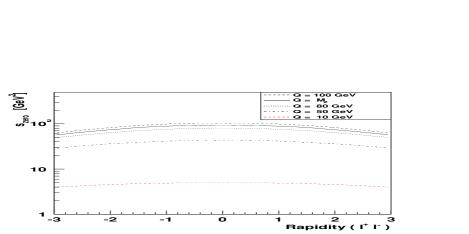
FIG. 4.: The dependence of $\mathrm{s}_{\mathrm{zero}}$ as a function of lepton-pair rapidity at several choices of parton the center-of-mass energy $Q$ is shown for the $p\bar{p}$ collisions at 2 TeV (Tevatron, top) and for $pp$ collisions at 14 TeV (LHC, bottom). The $\mathrm{s}_{\mathrm{zero}}$ function does not depend strongly on the vector-boson decay angles.

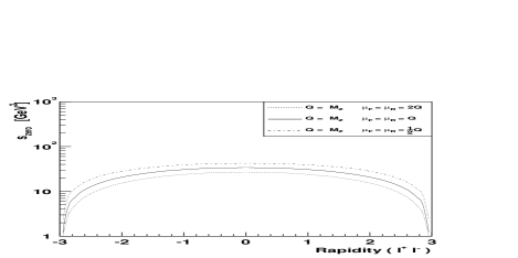
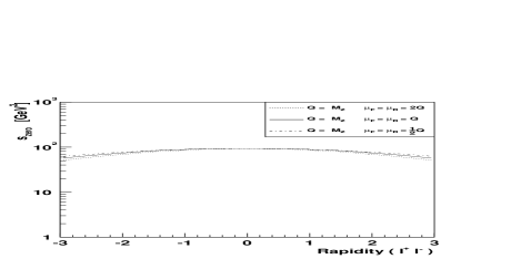
FIG. 5.: The scale variation of the $\mathrm{s}_{\mathrm{zero}}$ function evaluated at parton center-of-mass energy equal to the $Z^{0}$ mass is shown for $p\bar{p}$ collisions at 2 TeV (Tevatron, top) and for $pp$ collisions at 14 TeV (LHC, bottom). The $\mathrm{s}_{\mathrm{zero}}$ function encodes information about the factorization and renormalization scale choices into the $\Phi$-space Veto method, preserving the NLO calculation’s reduced scale dependence.

FIG. 6.: The inclusive NLO cross section for $p\bar{p}\rightarrow Z^{0}+X\rightarrow e^{+}e^{-}+X$ reactions at 2 TeV with the lepton-pair mass restricted to 66-116 GeV is shown as a function of the $\mathrm{s}_{\mathrm{min}}$ parameter for the $\mathrm{s}_{\mathrm{min}}$-slicing method. The cross section calculated using the $\Phi$-space Veto event generator is superimposed and is in good agreement. The Born-level cross section is also shown.

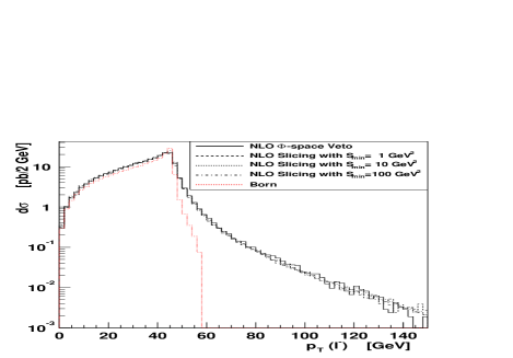
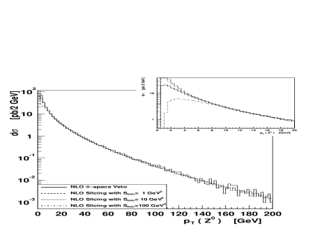
FIG. 7.: The transverse momentum of the electron (top) and vector-boson (bottom) are shown for the process $p\bar{p}\rightarrow Z^{0}+X\rightarrow e^{+}e^{-}+X$ at 2 TeV with the lepton-pair mass restricted to 66-116 GeV (no parton showering is used). Distributions derived from numerical integrations at NLO using $\mathrm{s}_{\mathrm{min}}$-slicing for various choices of the $\mathrm{s}_{\mathrm{min}}$ parameter are compared to the distributions from the NLO $\Phi$-space Veto event generator. Agreement is excellent everywhere, except in the low $P^{T}_{\mathrm{Z}}$ region (inset) where fixed order perturbative QCD is unreliable. The Born level prediction is also super-imposed for the $P^{T}_{\mathrm{e^{-}}}$ distribution (top). The Born level prediction for the vector-boson transverse momentum is a delta function at $P^{T}_{\mathrm{Z}}=0$.

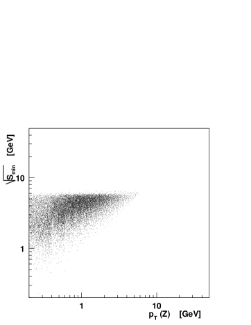
FIG. 8.: The kinematics of $\Phi$-space Veto method event candidates which have been veto-ed because they lie below the $\mathrm{s}_{\mathrm{zero}}$ boundary are plotted in the $P^{T}_{\mathrm{Z}}$ vs. $\sqrt{\mathrm{s}_{\mathrm{min}}}$ plane. The largest $P^{T}_{\mathrm{Z}}$ of a veto-ed candidate event is 5.5 GeV. The process is $p\bar{p}\rightarrow Z^{0}+X\rightarrow l^{+}l^{-}+X$ at 2 TeV with the lepton-pair mass restricted to 66-116 GeV.

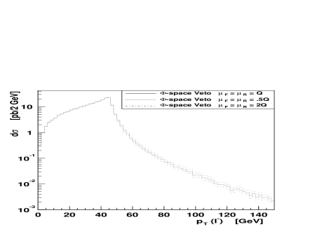
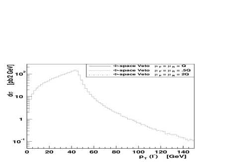
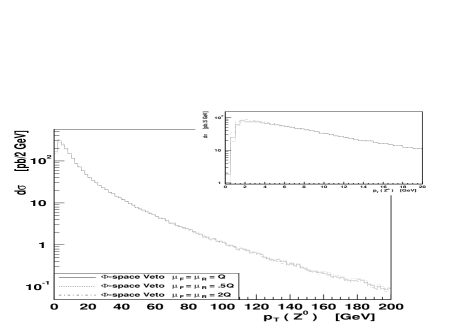
FIG. 9.: The transverse momentum of the electron (top) and vector-boson (bottom) are shown for the process $p\bar{p}\rightarrow Z^{0}+X\rightarrow e^{+}e^{-}+X$ at NLO using the $\Phi$-space Veto method (no parton showering is used) for different choices of the renormalization and factorization scales. The spread in the distributions is an indication of the theoretical error from neglected higher order terms. The distributions on the left are for 2 TeV $p\bar{p}$ collisions at the Tevatron, and the ones on the right are for 14 TeV $pp$ collisions at the LHC. The lepton-pair mass is restricted to 66-116 GeV, and the three curves use the same event sample.

FIG. 10.: The reduced scale dependence of the NLO $\Phi$-space Veto calculation as compared to the Born one is demonstrated. The transverse momentum of the electron (top) for the process $pp\rightarrow Z^{0}+X\rightarrow e^{+}e^{-}+X$ with the lepton-pair mass restricted to 66-116 GeV at LHC energy (14 TeV) is shown (the vector-boson transverse momentum is not shown because the Born level calculation does not provide a prediction for $P^{T}_{\mathrm{Z}}$). The renormalization and factorization scales are varied by a factor two in the Born level calculation (left) and the NLO $\Phi$-space Veto calculation (right). The percent variation of the distributions is shown at bottom. The variation is about a factor 4 smaller for the NLO $\Phi$-space Veto. The effect is smaller at Tevatron energy in this region.

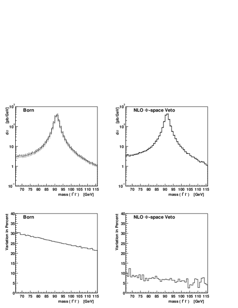
FIG. 11.: The reduced scale dependence of the NLO $\Phi$-space Veto calculation as compared to the Born one is demonstrated. The lepton-pair mass in the vicinity of the $Z^{0}$ resonance is shown (top) for the process $pp\rightarrow Z^{0}+X\rightarrow e^{+}e^{-}+X$ at LHC energy (14 TeV). The renormalization and factorization scales are varied by a factor two in the Born level calculation (left) and the NLO $\Phi$-space Veto calculation (right). The percent variation of the distributions is shown at bottom. The variation is about a factor 3 smaller for the NLO $\Phi$-space Veto. The effect is smaller at Tevatron energy.

FIG. 12.: A projection of the $pp\!\!\!\!^{{}^{(-)}}\rightarrow Z^{0}j$ phase space onto the $\hat{u}$ vs. $\hat{t}$ plane is shown, where $\hat{u}=(p_{2}-p_{j})^{2}=-Q^{2}_{2j}$ and $\hat{t}=(p_{1}-p_{j})^{2}=-Q^{2}_{1j}$, and $p_{1},~{}p_{2},~{}p_{j}$ are the momenta of the forward colliding parton, backward colliding parton, and the hardest emission. Events in the region of hard well separated partons are sampled with the first order matrix element, then evolved further by the parton shower. Events in the region between the $\mathrm{s}_{\mathrm{zero}}$ and $\mathrm{s}_{\mathrm{P.S.}}$ boundaries are projected onto n-body kinematics (i.e. onto the origin of the plane) and then evolved with the parton shower to a point which may lie anywhere below the $\mathrm{s}_{\mathrm{P.S.}}$ boundary. The region below $\mathrm{s}_{\mathrm{zero}}$ is never sampled, but may be reached by the projected and showered events.

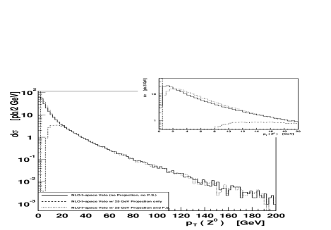
FIG. 13.: The $P^{T}_{\mathrm{Z}}$ distribution is shown after different stages of the event generation for $p\bar{p}\rightarrow Z^{0}+X\rightarrow e^{+}e^{-}+X$ at 2 TeV with the lepton-pair mass restricted to 66-116 GeV. The solid line is the $\Phi$-space Veto NLO distribution without any projection or parton shower. The dashed line is the (nonphysical) distribution for the same event sample, after applying the projection with $\sqrt{\mathrm{s}_{\mathrm{P.S.}}}=25$ GeV. The dotted line is the distribution after subsequent evolution through the showering and hadronization program.

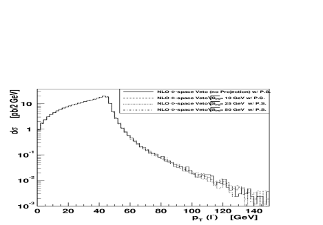
FIG. 14.: The effect of the parton shower on the $\Phi$-space Veto distributions is shown for several choices of the $\mathrm{s}_{\mathrm{P.S.}}$ parameter which partitions the phase space into the region populated by the parton shower, and the region populated directly by the first order matrix elements. The transverse momentum of the electron (top) and vector-boson (bottom) are plotted for the process $p\bar{p}\rightarrow Z^{0}+X\rightarrow e^{+}e^{-}+X$ at 2 TeV with the lepton-pair mass restricted to 66-116 GeV. There is very little dependence on the specific choice of the $\mathrm{s}_{\mathrm{P.S.}}$ parameter.

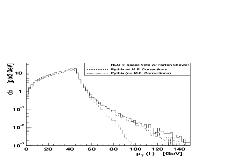
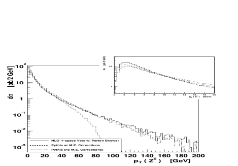
FIG. 15.: Distributions for the process $p\bar{p}\rightarrow Z^{0}+X\rightarrow e^{+}e^{-}+X$ at 2 TeV from the $\Phi$-space Veto event generator (solid line, includes evolution through the PYTHIA shower and hadronization program) are compared with the PYTHIA internal process distributions. The dashed line is the “matrix element corrected” PYTHIA prediction and the dotted line is the “old” (no matrix element corrections) PYTHIA prediction. The lepton-pair mass is restricted to 66-116 GeV.

TABLE I.: A comparison of computer processing time for the $\Phi$-space Veto method and for PYTHIA. In each case 10000 events are generated for the process $p\bar{p}\rightarrow Z^{0}+X\rightarrow e^{+}e^{-}+X$ at 2 TeV and the events are evolved through the PYTHIA shower and hadronization program. The $\Phi$-space Veto event generator requires some time to initialize the Bases/Spring grids (i.e. “learn the phase space”), whereas no initialization time is required for PYTHIA processes. The processing time per event and efficiency are similar. The computer is a 650 MHz Pentium III.

Method	Time for Grid Initialization	Time for 10000 Events	Efficiency
$\Phi$-space Veto	14.0 s	70.3 s	28%
PYTHIA	—	68.6 s	27%

REFERENCES

- [1] T. Sjöstrand, Phys. Lett. B157, 321 (1985).
- [2] G. Marchesini and B. R. Webber, Nucl. Phys. B310, 461 (1988).
- [3] T. Sjöstrand, P. Eden, C. Friberg, L. Lönnblad, G. Miu, S. Mrenna and E. Norrbin, Comput. Phys. Commun. 135, 238 (2001) [hep-ph/0010017]; T. Sjöstrand, L. Lönnblad and S. Mrenna, LU TP 01-21, [hep-ph/0108264].
- [4] G. Corcella et al., JHEP 0101, 010 (2001) [hep-ph/0011363].
- [5] H. Baer, F. E. Paige, S. D. Protopopescu and X. Tata, hep-ph/0001086.
- [6] J. Collins, arXiv:hep-ph/0110113; Y. Chen, J. C. Collins and N. Tkachuk, JHEP 0106, 015 (2001) [arXiv:hep-ph/0105291]; J. C. Collins, JHEP 0005, 004 (2000) [arXiv:hep-ph/0001040].
- [7] M. Dobbs and M. Lefebvre, Phys. Rev. D 63, 053011 (2001) [hep-ph/0011206].
- [8] M. Dobbs, Phys. Rev. D 64, 034016 (2001) [arXiv:hep-ph/0103174].
- [9] B. Pötter, Phys. Rev. D 63, 114017 (2001) [arXiv:hep-ph/0007172].
- [10] G. Altarelli, R. K. Ellis and G. Martinelli, Nucl. Phys. B 157, 461 (1979); J. Kubar-Andre and F. E. Paige, Phys. Rev. D 19, 221 (1979); K. Harada, T. Kaneko and N. Sakai, Nucl. Phys. B 155, 169 (1979) [Erratum-ibid. B 165, 545 (1979)]; J. Abad and B. Humpert, Phys. Lett. B 80, 286 (1979); J. Abad, B. Humpert and W. L. van Neerven, Phys. Lett. B 83, 371 (1979); B. Humpert and W. L. Van Neerven, Phys. Lett. B 84, 327 (1979) [Erratum-ibid. B 85, 471 (1979)]; B. Humpert and W. L. Van Neerven, Phys. Lett. B 85, 293 (1979).
- [11] U. Baur, O. Brein, W. Hollik, C. Schappacher and D. Wackeroth, arXiv:hep-ph/0108274.
- [12] R. K. Ellis, D. A. Ross and A. E. Terrano, Nucl. Phys. B178, 421 (1981).
- [13] S. Catani and M. H. Seymour, Nucl. Phys. B 485, 291 (1997) [Erratum-ibid. B 510, 503 (1997)] [arXiv:hep-ph/9605323].
- [14] L. J. Bergmann, Next-to-leading-log QCD calculation of symmetric dihadron production, Ph.D. thesis, Florida State University, 1989; H. Baer, J. Ohnemus and J. F. Owens, Phys. Rev. D40, 2844 (1989).
- [15] B. W. Harris and J. F. Owens, hep-ph/0102128.
- [16] K. Fabricius, I. Schmitt, G. Kramer and G. Schierholz, Z. Phys. C 11, 315 (1981); G. Kramer and B. Lampe, Fortsch. Phys. 37, 161 (1989).
- [17] W. T. Giele and E. W. Glover, Phys. Rev. D 46, 1980 (1992).
- [18] W. T. Giele, E. W. Glover and D. A. Kosower, Nucl. Phys. B 403, 633 (1993) [arXiv:hep-ph/9302225].
- [19] H. Baer and M. H. Reno, Phys. Rev. D 44, 3375 (1991); H. Baer and M. H. Reno, Phys. Rev. D 45, 1503 (1992).
- [20] B. Pötter and T. Schorner, Phys. Lett. B 517, 86 (2001) [arXiv:hep-ph/0104261].
- [21] E. W. Glover and M. R. Sutton, Phys. Lett. B 342, 375 (1995) [arXiv:hep-ph/9410234].
- [22] P. Aurenche and J. Lindfors, Nucl. Phys. B 185, 274 (1981). A factor is missing from the second term of Eq. 8 in this reference.
- [23] S. Kawabata, Comput. Phys. Commun. 88, 309 (1995). The C++ version is provided by private communication from the author.
- [24] H. L. Lai et al., Phys. Rev. D55, 1280 (1997) [hep-ph/9606399].
- [25] C. T. Davies, B. R. Webber and W. J. Stirling, Nucl. Phys. B 256, 413 (1985).
- [26] E. Boos et al., arXiv:hep-ph/0109068.
- [27] G. Corcella and M. H. Seymour, Phys. Lett. B442, 417 (1998) [hep-ph/9809451].
- [28] S. Catani, F. Krauss, R. Kuhn and B. R. Webber, arXiv:hep-ph/0109231; B. R. Webber, arXiv:hep-ph/0005035; F. Krauss, R. Kuhn and G. Soff, J. Phys. G 26, L11 (2000) [arXiv:hep-ph/9904274].
- [29] J. Andre and T. Sjöstrand, Phys. Rev. D 57, 5767 (1998) [arXiv:hep-ph/9708390].
- [30] F. Krauss, R. Kuhn and G. Soff, Acta Phys. Polon. B 30, 3875 (1999) [arXiv:hep-ph/9909572]; R. Kuhn, F. Krauss, B. Ivanyi and G. Soff, Comput. Phys. Commun. 134, 223 (2001) [arXiv:hep-ph/0004270].
- [31] G. Miu and T. Sjöstrand, Phys. Lett. B449, 313 (1999) [hep-ph/9812455]; T. Sjöstrand, hep-ph/0001032. In this reference the PYTHIA prediction is compared to experimental data. The authors realized after publication that the experimental data had not been unfolded from detector effects, and so any interpretations of the comparison should be made with this in mind.