Probing colored glass
via $q\bar{q}$ photoproduction
II: diffraction

Abstract

In this paper, we consider the diffractive photoproduction of quark-antiquark pairs in peripheral heavy ion collisions. The color field of the nuclei is treated within the Colored Glass Condensate model. The cross-section turns out to be very sensitive to the value of the saturation scale.

1. Laboratoire de Physique Téorique,
   Bât. 210, Université Paris XI,
   91405 Orsay Cedex, France

2. Brookhaven National Laboratory,
   Physics Department, Nuclear Theory,
   Upton, NY-11973, USA

BNL-NT-01/27, LPT-ORSAY-01-110

1 Introduction

In recent years, a lot of work has been devoted to the understanding of the parton distributions inside highly energetic hadrons or nuclei (see [1, 2] for a pedagogical introduction). A central question in this field is the issue of parton saturation at small values of the momentum fraction $x$ [3, 4, 5]. Indeed, the BFKL equation [6, 7, 8], when applied to extremely small values of $x$, leads to cross-sections that are too large to be compatible with unitarity constrains. It has been argued that this description becomes inadequate when non-linear effects in QCD become important, which happens when the phase-space density reaches the order of $1/\alpha_{s}$ [3, 9, 10, 11].

A theoretical description of saturation is provided by the model introduced by McLerran and Venugopalan [12, 13, 14], in which small-$x$ gluons inside a fast moving nucleus are described by a classical color field, which is motivated by the large occupation number of the corresponding modes. The color field is determined by the classical Yang-Mills equation with a current induced by the partons at large values of $x$. The distribution of hard color sources inside the nucleus is determined by a functional density which is assumed to be Gaussian in the original form of the model. This physical picture has been named “Colored Glass Condensate”. When quantum corrections are taken into account, the density distribution evolves according to a functional evolution equation [15, 16, 17, 18, 19, 20, 21, 22, 23, 24] which reduces in special cases to the BFKL equation. It is interesting to note that this evolution equation was recently reobtained in the dipole picture [25], which is the natural description in the frame where the nucleus is at rest.

The classical version of the color glass condensate model contains only one parameter, called “saturation scale” $Q_{s}$, and defined as the transverse momentum scale below which saturation effects start being important. This scale increases with energy and with the size of the nucleus [1, 9, 10]. Therefore, at energies high enough so that $Q_{s}\gg\Lambda_{{}_{QCD}}$, the coupling constant at the saturation scale is small, which makes perturbative approaches feasible.

Note that another model inspired by saturation has also been developed by Golec-Biernat and Wusthoff in order to fit the HERA data [26, 27]. There, saturation is included via a phenomenological formula for the dipole cross-section $\sigma(r_{\perp})=\sigma_{0}(1-\exp(-r_{\perp}^{2}/R(x)^{2}))$ that saturates for large dipole sizes. The radius $R(x)$ is the dipole size above which the saturation occurs, and is taken to be of the form $R(x)=(x/x_{0})^{\lambda/2}$GeV^-1. A fit to inclusive data at small $x$ gave $\sigma_{0}=23$mb, $x_{0}=3.10^{-4}$ and $\lambda=0.29$. This phenomenological model has also been successfully applied to the description of diffractive HERA data [28]. The main differences between this model and the colored glass condensate model are two-fold: in the model by Golec-Biernat and Wusthoff, saturation is introduced by hand, and the $x$ evolution of the saturation scale is also ad hoc. In the colored glass condensate, saturation emerges explicitly as a consequence of solving the fully non-linear classical Yang-Mills equations, and the quantum evolution is described by an evolution equation that may lead in principle to an $x$ dependence much more complicated than a power law. One may also note the attempts [29, 30] to fill the gap between the phenomenological approach of Golec-Biernat and Wusthoff and perturbative QCD, by using perturbative QCD as a starting point and adding shadowing corrections a la Glauber-Mueller.

Saturation effects, and in particular the color glass condensate model can be tested in deep inelastic scattering experiments by measuring structure functions like $F_{2}$ [31]. Interestingly, it also leads to potentially observable effects in the field of heavy ion collisions. For central collisions, the colored glass condensate model has been used to compute the distribution of the gluons produced initially, both analytically [32, 33, 34] and numerically on a 2-dimensional lattice [35, 36]. This initial gluon multiplicity is expected to control directly the observed final multiplicity. Recently, we have shown [37] that the parton saturation leads to interesting effects also in peripheral collisions, where it can be probed via the photoproduction of quark-antiquark pairs. In particular, the saturation scale $Q_{s}$ controls directly the position of the maximum in the transverse momentum spectrum of the pairs.

The present paper is an extension of this previous work, where we study the diffractive photoproduction of quark-antiquark pairs in peripheral heavy ion collisions. By diffractive production, we mean events in which the nuclei remain intact, and with a rapidity gap between the nuclei and the produced objects characterizing the topology of the final state. This implies that the exchange between the color field and the quark pair is color singlet, and carries a vanishing total transverse momentum. The simplest diagram for this process is represented in figure 1.

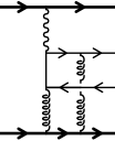
Figure 1: Prototype of the diagrams contributing to the diffractive photoproduction of a $q\bar{q}$ pair in $AA$ collisions.

We consider large ultra-relativistic nuclei, and we take into account the electromagnetic interaction to lowest order in the coupling (or, equivalently, in the leading logarithmic approximation), and the interactions with the strong color background field to all orders. We find that the cross-section of this process is very sensitive to the value of the saturation scale in the colored glass condensate. Note that we use a Gaussian distribution in order to describe the hard color sources that are generating the classical color fields. This means that no quantum evolution has been included in this calculation. It is known that in the colored glass condensate model, the quantum corrections lead to a modification of the distribution function of hard sources when the energy increases [15, 16, 17, 18, 19, 20, 21, 22, 23, 24] (a similar evolution equation has been derived by Kovchegov and Levin in the dipole language [38], and has been recently shown to be equivalent to the evolution equation in the colored glass condensate by Mueller [25]). In general, this distribution will not keep a Gaussian form due to these corrections. However, in order to assess very simply saturation effects in diffractive ultra-peripheral collisions, we do not include this refinement here. Note that in principle, extending our calculation to include quantum evolution is just a matter of changing the correlator $\left<U(0)U^{\dagger}({\tenimbf x}_{\perp})\right>_{\overline{\rho}}$ that appears in our results (see Eq. (33) for instance) and contains all the information about the properties of the colored glass condensate by one that has been calculated with the evolved distribution of “hard sources”.

The structure of this paper is as follows. In section 2, we summarize results relevant for the calculation of particle production in a classical background field. We also recall how to calculate diffractive quantities in the McLerran-Venugopalan model. In section 3, we compute the pair production amplitude to lowest order in the electromagnetic coupling constant. In section 4, an expression for the transverse momentum spectrum of the components of the pair is derived, and in section 5 results for the integrated diffractive cross-section are presented. Finally, section 6 is devoted to concluding remarks.

2 Reduction formulas for pair production

In this section, we remind the reader of reduction formulas one can use to compute various physical quantities in a classical background field. The formalism was derived in [39], and here we are only going to recall the results, using similar notations. Different from the situation studied in [39], the relevant classical background field is now a superposition of an electromagnetic field and a color field. The color field is associated to the covariant gauge distribution of hard sources $\widetilde{\rho}$ (see section 2 of [37]). In order to calculate physical quantities, one has to average over an ensemble distribution of these sources. Quantities obtained before averaging over the sources will be denoted by an index $\widetilde{\rho}$.

2.1 $\overline{n}$ versus $P_{1}$

Certain quantities of interest for the problem of quark-antiquark production in a background field can be related to quark propagators with different boundary conditions in this background field [39]. The main results are the following.

The probability to produce exactly one $q\bar{q}$ pair in a background field can be related to the Feynman (or time-ordered) propagator of a quark via

$$P_{1}[\widetilde{\rho}]=|\left<0_{\rm out}|0_{\rm in}\right>_{[\widetilde{\rho}]}|^{2}\,\int{{d^{3}{\tenimbf q}}\over{(2\pi)^{3}2\omega_{\tenimbf q}}}{{d^{3}{\tenimbf p}}\over{(2\pi)^{3}2\omega_{\tenimbf p}}}\left|\overline{u}({\tenimbf q}){\cal T}_{F}^{[\widetilde{\rho}]}(q,-p)v({\tenimbf p})\right|^{2}\;.$$ (1)

In this equation, ${\cal T}_{F}^{[\widetilde{\rho}]}$ is the interacting part of the Feynman propagator of a quark in the background field generated by the source $\widetilde{\rho}$. In terms of the exact Feynman propagator $G_{F}^{[\widetilde{\rho}]}$ and the free Feynman propagator $G_{F}^{0}$, it is defined as

$$G_{F}^{[\widetilde{\rho}]}=G_{F}^{0}+G_{F}^{0}{\cal T}_{F}^{[\widetilde{\rho}]}G_{F}^{0}\;.$$ (2)

Note in Eq. (1) the presence of the square of the vacuum-to-vacuum amplitude $\left<0_{\rm out}|0_{\rm in}\right>_{[\widetilde{\rho}]}$, which is essential for the unitarity of the result.

Conversely, the average number of $q\bar{q}$ pairs produced in a background field, $\bar{n}=\sum nP_{n}$, where $P_{n}$ are the production probabilities, can be expressed in terms of the interacting part of the retarded propagator of a quark in this background:

$$\overline{n}[\widetilde{\rho}]=\int{{d^{3}{\tenimbf q}}\over{(2\pi)^{3}2\omega_{\tenimbf q}}}{{d^{3}{\tenimbf p}}\over{(2\pi)^{3}2\omega_{\tenimbf p}}}\left|\overline{u}({\tenimbf q}){\cal T}_{R}^{[\widetilde{\rho}]}(q,-p)v({\tenimbf p})\right|^{2}\;.$$ (3)

Another difference to Eq. (1) is the absence of the vacuum-to-vacuum factor.

For the background field of two nuclei in peripheral collisions, an interesting aspect is that in the ultra-relativistic limit the retarded propagator has a much simpler structure than the Feynman propagator [39]. This enables one to write the retarded propagator of a quark explicitly, while this is not possible for the time-ordered one.

2.2 Diffractive and inclusive quantities

So far, we have given the expression for quantities that would be observed for the background field configuration associated to a specific source $\widetilde{\rho}$. However, this is not what is measured in experiments where quantities are usually averaged over many collisions. In the colored glass condensate model, this translates into an average over the sources, which are assumed to have a Gaussian distribution in the classical version of the model.

The prescription to average observables, like for instance $P_{1}$ or $\overline{n}$, over $\widetilde{\rho}$ is

$$\left<{\cal O}\right>_{\widetilde{\rho}}\equiv\int[d\widetilde{\rho}]w[\widetilde{\rho}]{\cal O}[\widetilde{\rho}]\;,$$ (4)

with the distribution

$$w[\widetilde{\rho}]\equiv\exp\left\{-\int dx^{-}d^{2}{\tenimbf x}_{\perp}{{\widetilde{\rho}_{a}(x^{-},{\tenimbf x}_{\perp})\widetilde{\rho}^{a}(x^{-},{\tenimbf x}_{\perp})}\over{2\mu^{2}(x^{-})}}\right\}\;.$$ (5)

This averaging procedure yields inclusive physical quantities, “inclusive” meaning here that the final state of the nucleus which interacts by its color field is not observed. For the present case of $q\bar{q}$ photoproduction, it means that the process under consideration is: $ZA\to Zq\bar{q}X$ (the nucleus interacting electromagnetically, denoted by $Z$, remains intact, while the other nucleus may fragment).

It was also noted that one can obtain a diffractive quantity (i.e. for events where the nucleus $A$ does not break up) by averaging the amplitude over the sources $\widetilde{\rho}$ before squaring it in order to get a probability. This procedure has been outlined in [40, 41] and justified in [10]. The difference between the two ways of performing the average is illustrated in figure 2, where the shaded blob indicates an average over the color sources.

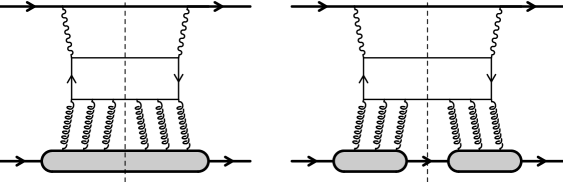
Figure 2: Inclusive (left) vs. diffractive (right) photoproduction of $q\bar{q}$ pairs. The shaded blob represents the average over a hard color source. For the diffractive cross-section, one has to average the amplitude before squaring it.

This average has the property that the gluons attached to one such blob carry a zero total transverse momentum and no net color. Given this, it is intuitive that the nucleus remains intact in the final state (i.e. on the cut represented by a dashed line) for the right diagram. In addition, this condition leads to a rapidity gap between the nucleus and the $q\bar{q}$ pair. More formal considerations on this issue can be found in [42].

Applied to the production of one $q\bar{q}$ pair, the inclusive probability is given by

$$P_{1}^{\rm incl}=\int{{d^{3}{\tenimbf q}}\over{(2\pi)^{3}2\omega_{\tenimbf q}}}{{d^{3}{\tenimbf p}}\over{(2\pi)^{3}2\omega_{\tenimbf p}}}\left<|\left<0_{\rm out}|0_{\rm in}\right>_{[\widetilde{\rho}]}|^{2}\,\left|\,\overline{u}({\tenimbf q}){\cal T}_{F}^{[\widetilde{\rho}]}(q,-p)v({\tenimbf p})\right|^{2}\right>_{\widetilde{\rho}}\;.$$ (6)

Note that the vacuum-to-vacuum factor must be included inside the average, because it depends on the source $\widetilde{\rho}$. On the other hand, the diffractive probability is given by

$$P_{1}^{\rm diff}=\int{{d^{3}{\tenimbf q}}\over{(2\pi)^{3}2\omega_{\tenimbf q}}}{{d^{3}{\tenimbf p}}\over{(2\pi)^{3}2\omega_{\tenimbf p}}}\left|\left<\left<0_{\rm out}|0_{\rm in}\right>_{[\widetilde{\rho}]}\overline{u}({\tenimbf q}){\cal T}_{F}^{[\widetilde{\rho}]}(q,-p)v({\tenimbf p})\right>_{\widetilde{\rho}}\right|^{2}\;.$$ (7)

Regarding, on the other hand, the average number of pairs in diffractive events, it is important to realize that this quantity cannot be obtained from the expression (3), which is already a combination of probabilities (i.e. squared amplitudes). From Eq. (3), therefore, only the average number of pairs produced in a collision, regardless of what happens to the nucleus, can be calculated [37]. In the rest of this paper, we focus on the calculation of $P_{1}^{\rm diff}$.

3 Expression of $P_{1}$ to order $(Z\alpha)^{2}$

The results of the previous section are valid to all orders in the coupling constants occurring in the problem, in particular the electromagnetic coupling $Z\alpha e_{q}$ of a quark with charge $e_{q}$ (in units of the positron charge) to the nucleus with atomic number $Z$. However, the Feynman propagator and the vacuum-to-vacuum amplitude are not known to all orders in $Z\alpha$, even in the ultra-relativistic limit (see [39]). In this section, we show that results can be obtained in closed form if one works at the lowest non-trivial order in $Z\alpha$, but to all orders in the interactions with the strong color field of the other nucleus. Although the value of $Z\alpha$ might seem too large ($Z\alpha\approx 0.6$ for a gold nucleus) as a useful expansion parameter, it turns out that at leading order the production probabilities contain large logarithms whose argument is the center of mass energy of the collision. It can be shown that higher order terms in $Z\alpha$ are suppressed by at least one power of this large logarithm, which justifies the approximation for large enough collision energies.

3.1 Pair production amplitude

Many simplifications occur when one considers only the leading order in $Z\alpha$. Indeed, since

$$\left|\overline{u}({\tenimbf q}){\cal T}_{F}^{[\widetilde{\rho}]}(q,-p)v({\tenimbf p})\right|^{2}={\cal O}((Z\alpha)^{2})\;,$$

$$|\left<0_{\rm out}|0_{\rm in}\right>_{\widetilde{\rho}}|^{2}=1+{\cal O}((Z\alpha)^{2})\;,$$ (8)

one can approximate the vacuum-to-vacuum factor by $1$ in the expression for $P_{1}$ at leading order in $Z\alpha$. Another notable simplification occurs in the Feynman propagator of the quark in the background field. From an infinite series, it simplifies to the sum of only three terms that are represented in figure 3. The interaction with the color field of the second nucleus is accounted for to all orders by eikonal factors depicted by the black dot.

Figure 3: The three diagrams contributing to ${\cal T}_{F}$ at lowest order in the electromagnetic coupling constant. The black dot denotes the time-ordered eikonal matrix $T_{F}$ that describes the interaction of a quark or antiquark with the colored glass condensate.

Thus, one can explicitly write down the time-ordered scattering matrix ${\cal T}_{F}^{[\widetilde{\rho}]}$ in terms of the individual scattering matrices off the two nuclei. The sum of the three diagrams of figure 3 is formally

$${\cal T}_{F}^{[\widetilde{\rho}]}=T_{F}^{{}^{QCD}}G_{F}^{0}T_{F}^{{}^{QED}}+T_{F}^{{}^{QED}}G_{F}^{0}T_{F}^{{}^{QCD}}+T_{F}^{{}^{QCD}}G_{F}^{0}T_{F}^{{}^{QED}}G_{F}^{0}T_{F}^{{}^{QCD}}\;,$$ (9)

where $G_{F}^{0}$ is the free time-ordered quark propagator:

$$G_{F}^{0}(p)=i{{\raise 0.43057pt\hbox{$/$}\kern-6.30005pt\hbox{$p$}+m}\over{p^{2}-m^{2}+i\epsilon}}\;.$$ (10)

$T_{F}^{{}^{QCD}}$ is the time-ordered scattering matrix of a quark in the color field of the second nucleus:

$$T_{F}^{{}^{QCD}}(q,p)=2\pi\delta(p^{-}-q^{-})\raise 0.43057pt\hbox{$/$}\kern-6.30005pt\hbox{$v$}_{+}{\rm sign}(p^{-})\int d^{2}{\tenimbf x}_{\perp}\left[U({\tenimbf x}_{\perp})^{{\rm sign}(p^{-})}-1\right]e^{i({\tenimbf q}_{\perp}-{\tenimbf p}_{\perp})\cdot{\tenimbf x}_{\perp}}$$ (11)

with

$$U({\tenimbf x}_{\perp})\equiv{\rm T}\exp\left\{-ig^{2}\int_{-\infty}^{+\infty}dz^{-}{1\over{\nabla_{\perp}^{2}}}\widetilde{\rho}_{a}(z^{-},{\tenimbf x}_{\perp})t^{a}\right\}\;,$$ (12)

where the $t^{a}$’s are the generators of the fundamental representation of $SU(N)$. At lowest order in $Z\alpha$, the scattering matrix of the quark in the electromagnetic field of the first nucleus simplifies to

$$T_{F}^{{}^{QED}}(q,p)=2\pi\delta(p^{+}-q^{+})\raise 0.43057pt\hbox{$/$}\kern-6.30005pt\hbox{$v$}_{-}{{4\pi Z\alpha e_{q}}\over{({\tenimbf q}_{\perp}-{\tenimbf p}_{\perp})^{2}}}e^{i({\tenimbf q}_{\perp}-{\tenimbf p}_{\perp})\cdot{\tenimbf b}}\;,$$ (13)

where ${\tenimbf b}$ is the impact parameter in the collision of the two nuclei (we chose the origin of coordinates in the transverse plane so that all the ${\tenimbf b}$ dependence goes into the electromagnetic scattering matrix).

From there, it is easy to work out a compact expression for the amplitude to create a $q\bar{q}$ pair by photoproduction in a peripheral collision. Replacing by $1$ the factor $\left<0_{\rm in}|0_{\rm out}\right>_{[\widetilde{\rho}]}$ at this order in $Z\alpha$, this amplitude is

$$M_{1}^{[\widetilde{\rho}]}({\tenimbf p},{\tenimbf q})=\overline{u}({\tenimbf q}){\cal T}_{F}^{[\widetilde{\rho}]}(q,-p)v({\tenimbf p})\;.$$ (14)

For the first two terms in Eq. (9), all the integrals over the $\pm$ components of the momentum transfer can be done thanks to the delta functions present in the individual scattering matrices. For the third term, there are two independent transfer momenta. Three of the $\pm$ integrals can still be performed with the delta functions, and the fourth one can be calculated in the complex plane with the theorem of residues. We obtain:

$$\!\!\!\!\!\!M_{1}^{[\widetilde{\rho}]}({\tenimbf p},{\tenimbf q})=$$

$$i\int{{d^{2}{\tenimbf k}_{\perp}}\over{(2\pi)^{2}}}F^{{}^{QED}}({\tenimbf p}_{\perp}+{\tenimbf q}_{\perp}-{\tenimbf k}_{\perp})F^{{}^{QCD}}_{+}({\tenimbf k}_{\perp}){{\overline{u}({\tenimbf q})\raise 0.43057pt\hbox{$/$}\kern-6.30005pt\hbox{$v$}_{+}(\raise 0.43057pt\hbox{$/$}\kern-6.30005pt\hbox{$q$}-\raise 0.6458pt\hbox{$/$}\kern-5.29999pt\hbox{$k$}+m)\raise 0.43057pt\hbox{$/$}\kern-6.30005pt\hbox{$v$}_{-}v({\tenimbf p})}\over{2p^{+}q^{-}+({\tenimbf q}_{\perp}-{\tenimbf k}_{\perp})^{2}+m^{2}}}$$

$$\!\!\!\!+i\int{{d^{2}{\tenimbf k}_{\perp}}\over{(2\pi)^{2}}}F^{{}^{QED}}({\tenimbf p}_{\perp}+{\tenimbf q}_{\perp}-{\tenimbf k}_{\perp})F^{{}^{QCD}}_{-}({\tenimbf k}_{\perp}){{\overline{u}({\tenimbf q})\raise 0.43057pt\hbox{$/$}\kern-6.30005pt\hbox{$v$}_{-}(\raise 0.6458pt\hbox{$/$}\kern-5.29999pt\hbox{$k$}-\raise 0.43057pt\hbox{$/$}\kern-6.30005pt\hbox{$p$}+m)\raise 0.43057pt\hbox{$/$}\kern-6.30005pt\hbox{$v$}_{+}v({\tenimbf p})}\over{2p^{-}q^{+}+({\tenimbf p}_{\perp}-{\tenimbf k}_{\perp})^{2}+m^{2}}}$$

$$\!\!\!\!+i\int{{d^{2}{\tenimbf k_{1}}_{\perp}}\over{(2\pi)^{2}}}{{d^{2}{\tenimbf k_{2}}_{\perp}}\over{(2\pi)^{2}}}F^{{}^{QED}}({\tenimbf p}_{\perp}+{\tenimbf q}_{\perp}-{\tenimbf k_{1}}_{\perp}-{\tenimbf k_{2}}_{\perp})F^{{}^{QCD}}_{+}({\tenimbf k_{1}}_{\perp})F^{{}^{QCD}}_{-}({\tenimbf k_{2}}_{\perp})$$

$$\qquad\qquad\times{{{\overline{u}({\tenimbf q})\raise 0.43057pt\hbox{$/$}\kern-6.30005pt\hbox{$v$}_{+}(\raise 0.43057pt\hbox{$/$}\kern-6.30005pt\hbox{$q$}-\raise 0.6458pt\hbox{$/$}\kern-5.29999pt\hbox{$k$}_{1}+m)\raise 0.43057pt\hbox{$/$}\kern-6.30005pt\hbox{$v$}_{-}(\raise 0.6458pt\hbox{$/$}\kern-5.29999pt\hbox{$k$}_{2}-\raise 0.43057pt\hbox{$/$}\kern-6.30005pt\hbox{$p$}+m)\raise 0.43057pt\hbox{$/$}\kern-6.30005pt\hbox{$v$}_{+}v({\tenimbf p})}\over{2q^{-}(({\tenimbf p}_{\perp}-{\tenimbf k_{2}}_{\perp})^{2}+m^{2})+2p^{-}(({\tenimbf q}_{\perp}-{\tenimbf k_{1}}_{\perp})^{2}+m^{2})}}}\;,$$ (15)

where we denote

$$F^{{}^{QED}}({\tenimbf k}_{\perp})\equiv{{4\pi Z\alpha}\over{{\tenimbf k}_{\perp}^{2}}}e^{i{\tenimbf k}_{\perp}\cdot{\tenimbf b}}\;,$$

$$F^{{}^{QCD}}_{\pm}({\tenimbf k}_{\perp})\equiv\int d^{2}{\tenimbf x}_{\perp}e^{i{\tenimbf k}_{\perp}\cdot{\tenimbf x}_{\perp}}\Big{(}U^{\pm 1}({\tenimbf x}_{\perp})-1\Big{)}\;.$$ (16)

At this stage, it is a simple matter of algebra to combine the three terms into a single one:

$$\!\!\!\!\!\!M_{1}^{[\widetilde{\rho}]}({\tenimbf p},{\tenimbf q})=$$

$$i\int{{d^{2}{\tenimbf k_{1}}_{\perp}}\over{(2\pi)^{2}}}{{d^{2}{\tenimbf k_{2}}_{\perp}}\over{(2\pi)^{2}}}F^{{}^{QED}}({\tenimbf p}_{\perp}+{\tenimbf q}_{\perp}-{\tenimbf k_{1}}_{\perp}-{\tenimbf k_{2}}_{\perp})$$

$$\!\!\!\!\!\!\times\int d^{2}{\tenimbf x_{1}}_{\perp}d^{2}{\tenimbf x_{2}}_{\perp}e^{i{\tenimbf k_{1}}_{\perp}\cdot{\tenimbf x_{1}}_{\perp}}e^{i{\tenimbf k_{2}}_{\perp}\cdot{\tenimbf x_{2}}_{\perp}}\Big{[}U({\tenimbf x_{1}}_{\perp})U^{\dagger}({\tenimbf x_{2}}_{\perp})-1\Big{]}M({\tenimbf p},{\tenimbf q}|{\tenimbf k_{1}}_{\perp},{\tenimbf k_{2}}_{\perp})\;,$$

(17)

where we define:

$$M({\tenimbf p},{\tenimbf q}|{\tenimbf k_{1}}_{\perp},{\tenimbf k_{2}}_{\perp})\equiv$$

$$\qquad\equiv\overline{u}({\tenimbf q}){{{\raise 0.43057pt\hbox{$/$}\kern-6.30005pt\hbox{$v$}_{+}(\raise 0.43057pt\hbox{$/$}\kern-6.30005pt\hbox{$q$}-\raise 0.6458pt\hbox{$/$}\kern-5.29999pt\hbox{$k$}_{1}+m)\raise 0.43057pt\hbox{$/$}\kern-6.30005pt\hbox{$v$}_{-}(\raise 0.6458pt\hbox{$/$}\kern-5.29999pt\hbox{$k$}_{2}-\raise 0.43057pt\hbox{$/$}\kern-6.30005pt\hbox{$p$}+m)\raise 0.43057pt\hbox{$/$}\kern-6.30005pt\hbox{$v$}_{+}}\over{2q^{-}(({\tenimbf p}_{\perp}-{\tenimbf k_{2}}_{\perp})^{2}+m^{2})+2p^{-}(({\tenimbf q}_{\perp}-{\tenimbf k_{1}}_{\perp})^{2}+m^{2})}}}v({\tenimbf p})\;.$$ (18)

This is the formula we will use in the following in order to compute the diffractive cross-section for the photoproduction of a quark-antiquark pair.

3.2 Equality of $P_{1}^{\rm incl}$ and $\overline{n}$ at order $(Z\alpha)^{2}$

Before going to the detailed calculation of the diffractive cross-section, it is interesting to check a property that holds at order $(Z\alpha)^{2}$. At this order, we have:

$$\overline{n}={\cal O}((Z\alpha)^{2})$$

$$P_{1}^{\rm incl}={\cal O}((Z\alpha)^{2})$$

$$P_{n}^{\rm incl}=0\qquad{\rm for\ }n\geq 2\;,$$ (19)

where $P_{n}^{\rm incl}$ is the inclusive probability to produce $n$ pairs in a collision. Since by definition $\overline{n}=P_{1}^{\rm incl}+2P_{2}^{\rm incl}+\cdots$, we immediately conclude that at order $(Z\alpha)^{2}$, one has $\overline{n}=P_{1}^{\rm incl}$. Although this property is obvious at such a formal level, it is interesting to see how it comes about in the explicit calculation. Indeed, we know that $\overline{n}$ is given by the square of a retarded amplitude, to which only the first two diagrams of figure 3 contribute [37], while all three diagrams contribute to $P_{1}^{\rm incl}$. The contribution of the first two diagrams to the retarded amplitude was calculated in [37],

$$\!\!\!\!\!\!M_{R}^{[\widetilde{\rho}]}({\tenimbf p},{\tenimbf q})=$$

$$-i\int{{d^{2}{\tenimbf k}_{\perp}}\over{(2\pi)^{2}}}F^{{}^{QED}}({\tenimbf p}_{\perp}+{\tenimbf q}_{\perp}-{\tenimbf k}_{\perp})\int d^{2}{\tenimbf x}_{\perp}e^{i{\tenimbf k}_{\perp}\cdot{\tenimbf x}_{\perp}}\Big{[}U({\tenimbf x}_{\perp})-1\Big{]}$$

$$\times\overline{u}({\tenimbf q})\Big{\{}{{\raise 0.43057pt\hbox{$/$}\kern-6.30005pt\hbox{$v$}_{+}(\raise 0.43057pt\hbox{$/$}\kern-6.30005pt\hbox{$q$}-\raise 0.6458pt\hbox{$/$}\kern-5.29999pt\hbox{$k$}+m)\raise 0.43057pt\hbox{$/$}\kern-6.30005pt\hbox{$v$}_{-}v({\tenimbf p})}\over{2p^{+}q^{-}+({\tenimbf q}_{\perp}-{\tenimbf k}_{\perp})^{2}+m^{2}}}+{{\raise 0.43057pt\hbox{$/$}\kern-6.30005pt\hbox{$v$}_{-}(\raise 0.6458pt\hbox{$/$}\kern-5.29999pt\hbox{$k$}-\raise 0.43057pt\hbox{$/$}\kern-6.30005pt\hbox{$p$}+m)\raise 0.43057pt\hbox{$/$}\kern-6.30005pt\hbox{$v$}_{+}v({\tenimbf p})}\over{2p^{-}q^{+}+({\tenimbf p}_{\perp}-{\tenimbf k}_{\perp})^{2}+m^{2}}}\Big{\}}v({\tenimbf p})\;.$$

After some algebra, this expression can be rewritten as

$$\!\!\!\!\!\!M_{R}^{[\widetilde{\rho}]}({\tenimbf p},{\tenimbf q})=$$

$$i\int{{d^{2}{\tenimbf k_{1}}_{\perp}}\over{(2\pi)^{2}}}{{d^{2}{\tenimbf k_{2}}_{\perp}}\over{(2\pi)^{2}}}F^{{}^{QED}}({\tenimbf p}_{\perp}+{\tenimbf q}_{\perp}-{\tenimbf k_{1}}_{\perp}-{\tenimbf k_{2}}_{\perp})$$

$$\times\int d^{2}{\tenimbf x_{1}}_{\perp}d^{2}{\tenimbf x_{2}}_{\perp}e^{i{\tenimbf k_{1}}_{\perp}\cdot{\tenimbf x_{1}}_{\perp}}e^{i{\tenimbf k_{2}}_{\perp}\cdot{\tenimbf x_{2}}_{\perp}}\Big{[}U({\tenimbf x_{1}}_{\perp})-U({\tenimbf x_{2}}_{\perp})\Big{]}M({\tenimbf p},{\tenimbf q}|{\tenimbf k_{1}}_{\perp},{\tenimbf k_{2}}_{\perp})\;.$$

Therefore, we see that at this order in $Z\alpha$, the time-ordered amplitude (17) and the retarded amplitude differ only by a factor $U({\tenimbf x_{2}}_{\perp})$ in the integrand. When squaring the amplitudes in order to get either $\overline{n}$ or $P_{1}^{\rm incl}$, this results in a factor $U({\tenimbf x_{2}}_{\perp})U^{\dagger}({\tenimbf x_{2}}^{\prime}_{\perp})$. Integrating over the transverse momentum ${\tenimbf p}_{\perp}$ of the antiquark yields $\delta({\tenimbf x_{2}}_{\perp}-{\tenimbf x_{2}}^{\prime}_{\perp})$, and this factor becomes unity ($U$ is a unitary matrix), leading to the expected equality $\overline{n}=P_{1}^{\rm incl}$.

3.3 A useful inequality

There is another very important property that we can prove without performing explicitly all the integrals. Performing only the integrals over ${\tenimbf p}_{\perp}$ and ${\tenimbf q}_{\perp}$, one can see that the eikonal color matrices present in the square of the time-ordered amplitude are of the form

$$\left<\Big{[}U({\tenimbf x_{1}}_{\perp})U^{\dagger}({\tenimbf x_{2}}_{\perp})-1\Big{]}\Big{[}U({\tenimbf x_{2}}_{\perp})U^{\dagger}({\tenimbf x_{1}}_{\perp})-1\Big{]}\right>_{\widetilde{\rho}}$$

$$\qquad\qquad=2\Big{[}1-\left<U({\tenimbf x_{1}}_{\perp})U^{\dagger}({\tenimbf x_{2}}_{\perp})\right>_{\widetilde{\rho}}\Big{]}$$ (22)

in the inclusive probability, and

$$\left<\Big{[}U({\tenimbf x_{1}}_{\perp})U^{\dagger}({\tenimbf x_{2}}_{\perp})-1\Big{]}\right>_{\widetilde{\rho}}\left<\Big{[}U({\tenimbf x_{2}}_{\perp})U^{\dagger}({\tenimbf x_{1}}_{\perp})-1\Big{]}\right>_{\widetilde{\rho}}$$

$$\qquad\qquad=\Big{[}1-\left<U({\tenimbf x_{1}}_{\perp})U^{\dagger}({\tenimbf x_{2}}_{\perp})\right>_{\widetilde{\rho}}\Big{]}^{2}$$ (23)

in the diffractive probability. In the above equations, we have used the fact that the correlator $\left<U({\tenimbf x_{1}}_{\perp})U^{\dagger}({\tenimbf x_{2}}_{\perp})\right>_{\widetilde{\rho}}$ is a real number, and symmetric under the exchange of the labels $1$ and $2$. All the other factors in the integrand are the same in both probabilities.

Recalling now the fact that $0\leq\left<U({\tenimbf x_{1}}_{\perp})U^{\dagger}({\tenimbf x_{2}}_{\perp})\right>_{\widetilde{\rho}}\leq 1$ (see the appendix of [37]), we also know that

$$\Big{[}1-\left<U({\tenimbf x_{1}}_{\perp})U^{\dagger}({\tenimbf x_{2}}_{\perp})\right>_{\widetilde{\rho}}\Big{]}^{2}\leq\Big{[}1-\left<U({\tenimbf x_{1}}_{\perp})U^{\dagger}({\tenimbf x_{2}}_{\perp})\right>_{\widetilde{\rho}}\Big{]}\;.$$ (24)

From this it is easy to infer the inequality

$$P_{1}^{\rm diff}\leq\frac{1}{2}\,P_{1}^{\rm incl}\,,$$ (25)

which will provide a useful consistency check at the end of the calculation. Using the fact that $\left<U({\tenimbf x_{1}}_{\perp})U^{\dagger}({\tenimbf x_{2}}_{\perp})\right>_{\widetilde{\rho}}$ vanishes in the limit $Q_{s}\to+\infty$, we also obtain from the above considerations

$$\lim_{Q_{s}\to+\infty}P_{1}^{\rm diff}={{P_{1}^{\rm incl}}\over 2}\;.$$ (26)

Therefore, the upper bound for $P_{1}^{\rm diff}$ (the ‘black-disc limit’) is reached for infinite $Q_{s}$, i.e. in the asymptotic limit where the center of mass energy of the collision is infinite.

4 $p_{\perp}$ spectrum for diffraction

We are now in a position to derive an expression for the quantity $P_{1}^{\rm diff}$. For this diffractive probability, we need to evaluate the average over the sources $\widetilde{\rho}$ of the amplitude $M_{1}^{[\widetilde{\rho}]}({\tenimbf p},{\tenimbf q})$. This involves the average $\left<U({\tenimbf x_{1}}_{\perp})U^{\dagger}({\tenimbf x_{2}}_{\perp})-1\right>_{\widetilde{\rho}}$, which was calculated in the appendix of [37],

$$\left<U({\tenimbf x_{1}}_{\perp})U^{\dagger}({\tenimbf x_{2}}_{\perp})-1\right>_{\widetilde{\rho}}$$

$$\qquad={\cal P}({\tenimbf x_{1}}_{\perp}){\cal P}({\tenimbf x_{2}}_{\perp})\Big{(}e^{-B_{2}({\tenimbf x_{1}}_{\perp}-{\tenimbf x_{2}}_{\perp})}-1\Big{)}$$

$$\qquad+({\cal P}({\tenimbf x_{1}}_{\perp})+{\cal P}({\tenimbf x_{2}}_{\perp})-2{\cal P}({\tenimbf x_{1}}_{\perp}){\cal P}({\tenimbf x_{2}}_{\perp}))\Big{(}e^{-B_{1}}-1\Big{)}\;.$$ (27)

Here the function ${\cal P}({\tenimbf x}_{\perp})$ describes the transverse profile of the nucleus (see [37] for more details on how it is introduced in the formalism). We assume ${\cal P}({\tenimbf x}_{\perp})=0$ outside the nucleus, and ${\cal P}({\tenimbf x}_{\perp})=1$ inside, and that for large nuclei the transition at the surface of the nucleus occurs over a distance much smaller than the nuclear radius $R$. In the above equation, we denote:

$$B_{2}({\tenimbf x}_{\perp}) \equiv Q_{s}^{2}\int d^{2}{\tenimbf z}_{\perp}[G_{0}({\tenimbf z}_{\perp})-G_{0}({\tenimbf z}_{\perp}-{\tenimbf x}_{\perp})]^{2}$$

$$\approx {{Q_{s}^{2}x_{\perp}^{2}}\over{4\pi}}\ln\left({1\over{x_{\perp}\Lambda_{{}_{QCD}}}}\right),$$

$$B_{1} \equiv Q_{s}^{2}\int d^{2}{\tenimbf z}_{\perp}G_{0}({\tenimbf z}_{\perp})^{2}\sim{{Q_{s}^{2}}\over{\Lambda_{{}_{QCD}}^{2}}}\gg 1$$ (28)

with $G_{0}({\tenimbf x}_{\perp})$ the 2-dimensional free propagator and where $Q_{s}$ is the saturation momentum. In the previous equations, one has to introduce by hand the scale $\Lambda_{{}_{QCD}}$ as a regulator for infrared singularities. More details on this can be found in [43].

In Eq. (27), the second term depends on ${\tenimbf x_{1}}_{\perp}$ and ${\tenimbf x_{2}}_{\perp}$ only via the profile function ${\cal P}$. Performing explicitly the integral over these coordinates, the contribution of this term to $\left<M_{1}^{[\widetilde{\rho}]}({\tenimbf p},{\tenimbf q})\right>_{\widetilde{\rho}}$ is:

$$i\int{{d^{2}{\tenimbf k_{1}}_{\perp}}\over{(2\pi)^{2}}}{{d^{2}{\tenimbf k_{2}}_{\perp}}\over{(2\pi)^{2}}}F^{{}^{QED}}({\tenimbf p}_{\perp}+{\tenimbf q}_{\perp}-{\tenimbf k_{1}}_{\perp}-{\tenimbf k_{2}}_{\perp})M({\tenimbf p},{\tenimbf q}|{\tenimbf k_{1}}_{\perp},{\tenimbf k_{2}}_{\perp})$$

$$\qquad\times\left(\widetilde{\cal P}({\tenimbf k_{1}}_{\perp})(2\pi)^{2}\delta({\tenimbf k_{2}}_{\perp})+\widetilde{\cal P}({\tenimbf k_{2}}_{\perp})(2\pi)^{2}\delta({\tenimbf k_{1}}_{\perp})-2\widetilde{\cal P}({\tenimbf k_{1}}_{\perp})\widetilde{\cal P}({\tenimbf k_{2}}_{\perp})\right)\;,$$

where the function $\widetilde{\cal P}({\tenimbf k}_{\perp})$ is the Fourier transform of the profile ${\cal P}({\tenimbf x}_{\perp})$. This function is strongly peaked around ${\tenimbf k}_{\perp}=0$, with a typical width of order $1/R$. Therefore, both ${\tenimbf k_{1}}_{\perp}$ and ${\tenimbf k_{2}}_{\perp}$ are at most of the order of $1/R$ in this integral. Since the factor $M({\tenimbf p},{\tenimbf q}|{\tenimbf k_{1}}_{\perp},{\tenimbf k_{2}}_{\perp})$ does not contain any scale as small as $1/R$ (this amplitude is controlled by the scale of the quark mass $m$), it is legitimate to replace it by the constant $M({\tenimbf p},{\tenimbf q}|0,0)$. By choosing ${\tenimbf k}_{\perp}\equiv{\tenimbf k_{1}}_{\perp}+{\tenimbf k_{2}}_{\perp}$ as one of the integration variables, this contribution can be rewritten as

$$2iM({\tenimbf p},{\tenimbf q}|0,0)\int{{d^{2}{\tenimbf k}_{\perp}}\over{(2\pi)^{2}}}F^{{}^{QED}}({\tenimbf p}_{\perp}+{\tenimbf q}_{\perp}-{\tenimbf k}_{\perp})$$

$$\qquad\times\int{{d^{2}{\tenimbf k}^{\prime}_{\perp}}\over{(2\pi)^{2}}}\left(\widetilde{\cal P}({\tenimbf k}_{\perp})(2\pi)^{2}\delta({\tenimbf k}^{\prime}_{\perp})-\widetilde{\cal P}({\tenimbf k}_{\perp})\widetilde{\cal P}({\tenimbf k}_{\perp}-{\tenimbf k}^{\prime}_{\perp})\right)\;.$$

At this point, it is trivial to see that the function of ${\tenimbf k}_{\perp}$ appearing on the second line of the previous expression is vanishing if we have ${\cal P}({\tenimbf x}_{\perp}){\cal P}({\tenimbf x}_{\perp})\approx{\cal P}({\tenimbf x}_{\perp})$. This is indeed the case if the transition of ${\cal P}({\tenimbf x}_{\perp})$ from 0 to 1 is sharp, i.e. if we can neglect surface effects in the description of the nucleus. To recapitulate, one can drop the second term of Eq. (27) if we have $m\gg 1/R$ and $R\gg\Lambda_{{}_{QCD}}^{-1}$.

For the remaining term, it is convenient to resort to an approximation already used in [37], valid when $Q_{s}\gg\Lambda_{{}_{QCD}}\gg 1/R$:

$${\cal P}({\tenimbf x_{1}}_{\perp}){\cal P}({\tenimbf x_{2}}_{\perp})e^{-B_{2}({\tenimbf x_{1}}_{\perp}-{\tenimbf x_{2}}_{\perp})}\approx{\cal P}({\tenimbf x_{1}}_{\perp})e^{-B_{2}({\tenimbf x_{1}}_{\perp}-{\tenimbf x_{2}}_{\perp})}\;.$$ (31)

This approximation just indicates that due to the factor $\exp(-B_{2})$ the difference ${\tenimbf x_{1}}_{\perp}-{\tenimbf x_{2}}_{\perp}$ is much smaller than the nuclear radius. Additionally, using the same arguments as above, the term ${\cal P}({\tenimbf x_{1}}_{\perp}){\cal P}({\tenimbf x_{2}}_{\perp})$ can be replaced by a single factor ${\cal P}({\tenimbf x_{1}}_{\perp})$. The Fourier transform of the first term of Eq. (27) is then trivial, as we have

$$\int d^{2}{\tenimbf x_{1}}_{\perp}d^{2}{\tenimbf x_{2}}_{\perp}e^{i{\tenimbf k_{1}}_{\perp}\cdot{\tenimbf x_{1}}_{\perp}}e^{i{\tenimbf k_{2}}_{\perp}\cdot{\tenimbf x_{2}}_{\perp}}{\cal P}({\tenimbf x_{1}}_{\perp})\left(e^{-B_{2}({\tenimbf x_{1}}_{\perp}-{\tenimbf x_{2}}_{\perp})}-1\right)$$

$$\qquad\qquad=\widetilde{\cal P}({\tenimbf k_{1}}_{\perp}+{\tenimbf k_{2}}_{\perp})(C({\tenimbf k_{2}}_{\perp})-(2\pi)^{2}\delta({\tenimbf k_{2}}_{\perp}))\;,$$ (32)

where, like in [37], we denote

$$C({\tenimbf k}_{\perp})\equiv\int d^{2}{\tenimbf x}_{\perp}e^{i{\tenimbf k}_{\perp}\cdot{\tenimbf x}_{\perp}}\left<U(0)U^{\dagger}({\tenimbf x}_{\perp})\right>_{\widetilde{\rho}}\;.$$ (33)

In the following, we use the notation

$$D({\tenimbf k}_{\perp})\equiv C({\tenimbf k}_{\perp})-(2\pi)^{2}\delta({\tenimbf k}_{\perp})\;.$$ (34)

To summarize, we have so far obtained a compact expression for the average of $M_{1}^{[\widetilde{\rho}]}$ that reads

$$\left<M_{1}^{[\widetilde{\rho}]}({\tenimbf p},{\tenimbf q})\right>_{\widetilde{\rho}}=i\int{{d^{2}{\tenimbf k_{1}}_{\perp}}\over{(2\pi)^{2}}}{{d^{2}{\tenimbf k_{2}}_{\perp}}\over{(2\pi)^{2}}}F^{{}^{QED}}({\tenimbf p}_{\perp}+{\tenimbf q}_{\perp}-{\tenimbf k_{1}}_{\perp}-{\tenimbf k_{2}}_{\perp})$$

$$\qquad\qquad\qquad\qquad\times\widetilde{\cal P}({\tenimbf k_{1}}_{\perp}+{\tenimbf k_{2}}_{\perp})D({\tenimbf k_{2}}_{\perp})M({\tenimbf p},{\tenimbf q}|{\tenimbf k_{1}}_{\perp},{\tenimbf k_{2}}_{\perp})\;.$$ (35)

Note that the factor $\widetilde{\cal P}({\tenimbf k_{1}}_{\perp}+{\tenimbf k_{2}}_{\perp})$ implies that the total momentum transfer ${\tenimbf k_{1}}_{\perp}+{\tenimbf k_{2}}_{\perp}$ from the nucleus acting via its color field is at most of order $1/R$, a feature that was to be expected for diffraction.

From here, we can proceed as in [37]. Since the photoproduction cross-section is enhanced by a factor $Z^{2}$ for photons that are produced coherently by the first nucleus, i.e. for photons with a transverse momentum ${\tenimbf p}_{\perp}+{\tenimbf q}_{\perp}-{\tenimbf k_{1}}_{\perp}-{\tenimbf k_{2}}_{\perp}$ smaller than $1/R$, we can perform a Taylor expansion of the factor $M({\tenimbf p},{\tenimbf q}|{\tenimbf k_{1}}_{\perp},{\tenimbf k_{2}}_{\perp})$ around the point where ${\tenimbf k_{1}}_{\perp}+{\tenimbf k_{2}}_{\perp}={\tenimbf p}_{\perp}+{\tenimbf q}_{\perp}$. Up to terms of higher order, this gives

$$M({\tenimbf p},{\tenimbf q}|{\tenimbf k_{1}}_{\perp},{\tenimbf k_{2}}_{\perp})\approx{{\overline{u}({\tenimbf q})\raise 0.43057pt\hbox{$/$}\kern-6.30005pt\hbox{$v$}_{+}v({\tenimbf p})}\over{p^{-}+q^{-}}}+({\tenimbf p}_{\perp}+{\tenimbf q}_{\perp}-{\tenimbf k_{1}}_{\perp}-{\tenimbf k_{2}}_{\perp})\cdot{\tenimbf L}({\tenimbf p},{\tenimbf q}|{\tenimbf k_{2}}_{\perp})\;,$$ (36)

with

$${\tenimbf L}({\tenimbf p},{\tenimbf q}|{\tenimbf k_{2}}_{\perp})\equiv{{1\over{(p^{-}+q^{-})(m^{2}+({\tenimbf k_{2}}_{\perp}-{\tenimbf p}_{\perp})^{2})}}}$$

$$\qquad\times\overline{u}({\tenimbf q})\Big{\{}{{2p^{-}}\over{p^{-}+q^{-}}}\raise 0.43057pt\hbox{$/$}\kern-6.30005pt\hbox{$v$}_{+}({\tenimbf k_{2}}_{\perp}-{\tenimbf p}_{\perp})+{{\raise 0.43057pt\hbox{$/$}\kern-6.30005pt\hbox{$v$}_{+}{\tenimbf\gamma}_{\perp}\raise 0.43057pt\hbox{$/$}\kern-6.30005pt\hbox{$v$}_{-}({\tenimbf k_{2}}_{\perp}-{\tenimbf p}_{\perp}+m)\raise 0.43057pt\hbox{$/$}\kern-6.30005pt\hbox{$v$}_{+}}\over{2}}\Big{\}}v({\tenimbf p})\;.$$

Thanks to the sum rule

$$\int{{d^{2}{\tenimbf k}_{\perp}}\over{(2\pi)^{2}}}\;D({\tenimbf k}_{\perp})=0\;,$$ (39)

the term of order zero in the expansion (36) does not contribute. Integrating over the photon momentum ${\tenimbf m}_{\perp}\equiv{\tenimbf p}_{\perp}+{\tenimbf q}_{\perp}-{\tenimbf k_{1}}_{\perp}-{\tenimbf k_{2}}_{\perp}$, while keeping ${\tenimbf k_{2}}_{\perp}$ fixed, leads to

$$\left<M_{1}^{[\widetilde{\rho}]}({\tenimbf p},{\tenimbf q})\right>_{\widetilde{\rho}}=2iZ\alpha e_{q}\widetilde{\cal P}({\tenimbf p}_{\perp}+{\tenimbf q}_{\perp})\int{{d^{2}{\tenimbf k}_{\perp}}\over{(2\pi)^{2}}}D({\tenimbf k}_{\perp}){{{\tenimbf b}\cdot{\tenimbf L}({\tenimbf p},{\tenimbf q}|{\tenimbf k}_{\perp})}\over{{\tenimbf b}^{2}}}\;.$$ (40)

Using then

$$\int d^{2}{\tenimbf b}{{{\tenimbf b}\cdot{\tenimbf L}({\tenimbf p},{\tenimbf q}|{\tenimbf k}_{\perp})}\over{{\tenimbf b}^{2}}}{{{\tenimbf b}\cdot{\tenimbf L}^{*}({\tenimbf p},{\tenimbf q}|{\tenimbf k}^{\prime}_{\perp})}\over{{\tenimbf b}^{2}}}={{{\tenimbf L}({\tenimbf p},{\tenimbf q}|{\tenimbf k}_{\perp})\cdot{\tenimbf L}^{*}({\tenimbf p},{\tenimbf q}|{\tenimbf k}^{\prime}_{\perp})}\over{2}}\int{{d^{2}{\tenimbf b}}\over{{\tenimbf b}^{2}}}$$ (41)

and

$$\widetilde{\cal P}^{2}({\tenimbf p}_{\perp}+{\tenimbf q}_{\perp})\approx\pi R^{2}(2\pi)^{2}\delta({\tenimbf p}_{\perp}+{\tenimbf q}_{\perp})\;,$$ (42)

we can write the diffractive cross-section for the photoproduction of a $q\bar{q}$ pair as

$$\sigma_{1}^{\rm diff} \equiv \int d^{2}{\tenimbf b}P_{1}^{\rm diff}=\pi R^{2}2N_{c}(Z\alpha)^{2}e_{q}^{2}\int\limits_{2R}^{\gamma/m}{{d^{2}{\tenimbf b}}\over{{\tenimbf b}^{2}}}$$ (43)

$$\times\int{{d^{3}{\tenimbf p}}\over{(2\pi)^{3}2\omega_{\tenimbf p}}}{{d^{3}{\tenimbf q}}\over{(2\pi)^{3}2\omega_{\tenimbf q}}}(2\pi)^{2}\delta({\tenimbf p}_{\perp}+{\tenimbf q}_{\perp})$$

$$\times\int{{d^{2}{\tenimbf k}_{\perp}}\over{(2\pi)^{2}}}{{d^{2}{\tenimbf k}^{\prime}_{\perp}}\over{(2\pi)^{2}}}D({\tenimbf k}_{\perp})D({\tenimbf k}^{\prime}_{\perp}){\rm Tr}\left({\tenimbf L}({\tenimbf p},{\tenimbf q}|{\tenimbf k}_{\perp})\cdot{\tenimbf L}^{*}({\tenimbf p},{\tenimbf q}|{\tenimbf k}^{\prime}_{\perp})\right).$$

In the integration over the impact parameter, the lower bound is determined by the geometry of a peripheral collision of two nuclei of radius $R$, and the upper bound is the limit beyond which the electromagnetic field does not have a Weizsäcker-Williams form. The calculation of the Dirac’s trace leads to

$${\rm Tr}\left({\tenimbf L}({\tenimbf p},{\tenimbf q}|{\tenimbf k}_{\perp})\cdot{\tenimbf L}^{*}({\tenimbf p},{\tenimbf q}|{\tenimbf k}^{\prime}_{\perp})\right)$$

$$\qquad={{16p^{-}q^{-}}\over{(p^{-}+q^{-})^{2}(m^{2}+({\tenimbf k}_{\perp}-{\tenimbf p}_{\perp})^{2})(m^{2}+({\tenimbf k}^{\prime}_{\perp}-{\tenimbf p}_{\perp})^{2})}}$$

$$\qquad\quad\times\Big{\{}m^{2}+({\tenimbf k}_{\perp}-{\tenimbf p}_{\perp})\cdot({\tenimbf k}^{\prime}_{\perp}-{\tenimbf p}_{\perp})\Big{[}1-2{{p^{-}}\over{p^{-}+q^{-}}}+2{{p^{-}{}^{2}}\over{(p^{-}+q^{-})^{2}}}\Big{]}\Big{\}}\;.$$

At this stage, it is straightforward to perform the integrals over $p^{\pm},q^{-}$ and ${\tenimbf q}_{\perp}$ in order to obtain the cross-section per unit of rapidity (we make use of $dq^{+}/q^{+}=2dy$):

$${{d\sigma_{1}^{\rm diff}}\over{dy}}=\pi R^{2}{{4N_{c}(Z\alpha)^{2}e_{q}^{2}}\over{\pi^{2}}}\int\limits_{2R}^{\gamma/m}{{d^{2}{\tenimbf b}}\over{{\tenimbf b}^{2}}}\int{{d^{2}{\tenimbf p}_{\perp}}\over{(2\pi)^{2}}}$$

$$\times\int{{d^{2}{\tenimbf k}_{\perp}}\over{(2\pi)^{2}}}{{d^{2}{\tenimbf k}^{\prime}_{\perp}}\over{(2\pi)^{2}}}D({\tenimbf k}_{\perp})D({\tenimbf k}^{\prime}_{\perp}){{m^{2}+{2\over 3}({\tenimbf k}_{\perp}-{\tenimbf p}_{\perp})\cdot({\tenimbf k}^{\prime}_{\perp}-{\tenimbf p}_{\perp})}\over{(m^{2}+({\tenimbf k}_{\perp}-{\tenimbf p}_{\perp})^{2})(m^{2}+({\tenimbf k}^{\prime}_{\perp}-{\tenimbf p}_{\perp})^{2})}}\;.$$

One can then note that the function $D({\tenimbf k}_{\perp})$ depends only on the radial variable $k_{\perp}$, and perform analytically all the angular integrals, which leads to the following formula for the $p_{\perp}$ spectrum of the quarks (or, equivalently, antiquarks) produced diffractively:

$${{d\sigma_{1}^{\rm diff}}\over{dydp_{\perp}}}=\pi R^{2}{{N_{c}(Z\alpha)^{2}e_{q}^{2}}\over{2\pi^{5}}}\int\limits_{2R}^{\gamma/m}{{d^{2}{\tenimbf b}}\over{{\tenimbf b}^{2}}}$$

$$\qquad\qquad\times p_{\perp}\,\left[m^{2}I_{1}^{2}+{1\over{6p_{\perp}^{2}}}(I_{2}-2p_{\perp}^{2}I_{1})^{2}\right]\;,$$ (46)

where we denote

$$I_{1}\equiv\int\limits_{0}^{+\infty}dk_{\perp}k_{\perp}D(k_{\perp}){1\over{\sqrt{(m^{2}+p_{\perp}^{2}+k_{\perp}^{2})^{2}-4p_{\perp}^{2}k_{\perp}^{2}}}}\;,$$

$$I_{2}\equiv\int\limits_{0}^{+\infty}dk_{\perp}k_{\perp}D(k_{\perp}){{m^{2}+p_{\perp}^{2}+k_{\perp}^{2}}\over{\sqrt{(m^{2}+p_{\perp}^{2}+k_{\perp}^{2})^{2}-4p_{\perp}^{2}k_{\perp}^{2}}}}\;.$$ (48)

Figure 4: Differential diffractive cross-section as a function of the transverse momentum of the quark. The value of $Q_{s}/\Lambda_{{}_{QCD}}$ is set to $10$. Open circles: strange quarks. Filled squares: charm quark. Open squares: bottom quark. The differential cross-section is in units of mbarns$/\Lambda_{{}_{QCD}}$.

Those two integrals are easy to evaluate numerically in order to obtain the $p_{\perp}$ spectrum of the produced quarks. Results are plotted in figure 4 for a value of $Q_{s}/\Lambda_{{}_{QCD}}=10$ (i.e. $Q_{s}\approx 2$GeV, if we assume $\Lambda_{{}_{QCD}}\approx 200$MeV) for strange ($m/\Lambda_{{}_{QCD}}\approx 1$), charm ($m/\Lambda_{{}_{QCD}}\approx 8$) and bottom ($m/\Lambda_{{}_{QCD}}\approx 23$) quarks. Corresponding to LHC collision energy, we chose a Lorentz factor of $\gamma=3000$, which is in the regime where the leading logarithm approximation is valid.

5 Integrated diffractive cross-section

5.1 Cross-section

The next step is to perform the integration over the transverse momentum of the produced quarks, in order to obtain total cross-sections or production probabilities. This can be done numerically, and the results are plotted in figure 5 as a function of $Q_{s}/\Lambda_{{}_{QCD}}$, for strange, charm, and bottom quarks. Again, the Lorentz factor is taken to be $\gamma=3000$.

Figure 5: Diffractive cross-section in mbarns per unit of rapidity as a function of the saturation scale. Open circles: strange quarks. Filled squares: charm quarks. Open squares: bottom quarks.

We can see that the cross-section for the production of $c\bar{c}$ and $b\bar{b}$ pairs is very sensitive to the value of the saturation scale $Q_{s}$, especially in the range $Q_{s}/\Lambda_{{}_{QCD}}\in[5,15]$. Therefore, this process could be used as a way to measure the saturation scale for ultra-relativistic heavy nuclei.

5.2 Unitarity and black-disc limit

It is interesting to investigate explicitly the inequality (25) between the diffractive $q\bar{q}$ production probability $P_{1}^{\rm diff}$ and the inclusive probability $P_{1}^{\rm incl}$ (which at leading order in $Z\alpha$ is equal to $\overline{n}$ calculated in [37]). The probability can easily be obtained from the expression for the respective cross-section by integrating over the rapidity, but without performing the integration over the impact parameter. Note that assuming $\gamma\rightarrow\infty$ in our present approach leads to a flat rapidity distribution, and a cutoff in rapidity must be introduced by hand. For the numerical calculation, we assume a rapidity range of $2\ln(\gamma)$, which leads to the relation

$$P_{1}^{\rm diff}(2R)=\ln\gamma\left[4\pi R^{2}\ln\frac{\gamma}{2mR}\right]^{-1}\frac{d\sigma_{1}^{\rm diff}}{dy}$$ (49)

between the probability at the smallest possible impact parameter and the cross-section. In figure 6, we have displayed $\overline{n}$, $\overline{n}/2$ and $P_{1}^{\rm diff}$, at $b=2R$ and for a Lorentz factor $\gamma=3000$, as functions of $Q_{s}/\Lambda_{{}_{QCD}}$ for strange and charm quarks.

Figure 6: Verification of the inequality $P_{1}^{\rm diff}\leq\overline{n}/2$ for the production of $q\bar{q}$ pairs at $b=2R$, as a function of $Q_{s}/\Lambda_{{}_{QCD}}$. Top: strange quarks; bottom: charm quarks. Filled squares: average multiplicity for inclusive events ($\overline{n}$); solid line: $\overline{n}/2$. Open squares: non-unitarized probability for the production of a $q\bar{q}$ pair in a diffractive event ($P_{1}^{\rm diff}$); dashed line: naive unitarization of this probability ($P_{1}^{\rm diff}\exp(-P_{1}^{\rm diff})$).

As expected, we always find $P_{1}^{\rm diff}\leq\overline{n}/2$. We also observe that the two quantities tend to a common value as $Q_{s}$ becomes large. Indeed, in the McLerran-Venugopalan model the black-disc limit corresponds to an infinitely large value of the saturation scale.

We have already emphasized the importance of the prefactor $\left<0_{\rm out}|0_{\rm in}\right>_{\widetilde{\rho}}$, to ensure that the obtained probabilities are smaller than $1$. However, in the present calculation, in which we have kept only the terms of lowest order in $Z\alpha$, this factor is approximated by $1$. Therefore, it is expected that this approximation violates unitarity, and that unitarity is restored by terms of higher order in the electromagnetic coupling. These corrections are rather difficult to calculate exactly. For a rough estimate of their size, we suppose that the diffractive multiplicities have a Poissonian distribution, and that the unitarized probability to create one pair diffractively is given by $P_{1}^{\rm diff}\exp(-P_{1}^{\rm diff})$. This expression is also plotted in figure 6. We see that the unitarization effects (i.e. the higher order corrections in $Z\alpha$) are not important as long as the average multiplicity is much smaller than one. In particular, we estimate that the unitarity corrections remain small in the range of values of $Q_{s}$ expected to be relevant at RHIC or at LHC (between $1$ and $3$GeV). We also emphasize the fact that this estimate has been done for the probabilities at the smallest allowed impact parameter $b=2R$, where the non-unitarized probabilities are the largest. Integrating the unitarized probability over the impact parameter for an estimate of the unitarization corrections in the diffractive cross-section, they are found to be smaller by a relative factor of $P_{1}^{\rm diff}(2R)/2\ln(\gamma/2mR)$. Hence, they can be neglected here.

5.3 Summary

To close this section, let us provide a table of the values of the cross-section per unit of rapidity, for charm and bottom quark pairs, and for inclusive and diffractive production:

	charm	bottom
$d\sigma_{\rm incl}/dy\ (\rm mb)$	355	11
$d\sigma_{\rm diff}/dy\ (\rm mb)$	60	0.62

Those numbers are obtained for a Lorentz factor $\gamma=3000$, a nuclear radius $R=6$fm and a saturation scale $Q_{s}=10\Lambda_{{}_{QCD}}$.

6 Conclusions

In this paper, we have evaluated the cross-section for the diffractive photoproduction of $q\bar{q}$ pairs in peripheral collisions of heavy nuclei. Diffractive events are particularly interesting because they could provide a cleaner final state due a rapidity gap between the nuclei and the pair. This process can be used as a way to test saturation models, and to measure the value of the saturation scale in heavy ion experiments. Indeed, the yield of $q\bar{q}$ pairs has been found to be very sensitive to the value of the saturation scale, especially for $c$ and $b$ quarks and for values of the saturation scale between $1$ and $3$GeV.

We have also checked that our result is consistent with the one obtained in [37] for the photoproduction of pairs in inclusive events. In particular, the inequality $P_{1}^{\rm diff}\leq P_{1}^{\rm incl}/2$ is satisfied by our calculation, and the black-disc limit is recovered when the saturation scale becomes infinite.

Acknowledgments: This work is supported by DOE under grant DE-AC02-98CH10886. A.P. is supported in part by the A.-v.-Humboldt foundation (Feodor-Lynen program). We would like to thank A. Dumitru, J. Jalilian-Marian, D. Kharzeev, L. McLerran, R. Venugopalan and U. Wiedemann for discussions on this problem.

References

- [1] A.H. Mueller, Lectures given at the International Summer School on Particle Production Spanning MeV and TeV Energies (Nijmegen 99), Nijmegen, Netherlands, 8-20, Aug 1999, hep-ph/9911289.
- [2] L. McLerran, Lectures given at the 40’th Schladming Winter School: Dense Matter, March 3-10 2001, hep-ph/0104285.
- [3] L.V. Gribov, E.M. Levin, M.G. Ryskin, Phys. Rept. 100, 1 (1983).
- [4] A.H. Mueller, J-W. Qiu, Nucl. Phys. B 268, 427 (1986).
- [5] L.L. Frankfurt, M.I. Strikman, Phys. Rept. 160, 235 (1988).
- [6] L.N. Lipatov, Sov. J. Nucl. Phys. 23, 338 (1976).
- [7] E.A. Kuraev, L.N. Lipatov, V.S. Fadin, Sov. Phys. JETP 45, 199 (1977).
- [8] I. Balitsky, L.N. Lipatov, Sov. J. Nucl. Phys. 28, 822 (1978).
- [9] J. Jalilian-Marian, A. Kovner, L. McLerran, H. Weigert, Phys. Rev. D 55, 5414 (1997).
- [10] Yu.V. Kovchegov, L. McLerran, Phys. Rev. D 60, 054025 (1999).
- [11] Yu.V. Kovchegov, L. McLerran, Erratum Phys. Rev. D 62, 019901 (2000).
- [12] L. McLerran, R. Venugopalan, Phys. Rev. D 49, 2233 (1994).
- [13] L. McLerran, R. Venugopalan, Phys. Rev. D 49, 3352 (1994).
- [14] L. McLerran, R. Venugopalan, Phys. Rev. D 50, 2225 (1994).
- [15] J. Jalilian-Marian, A. Kovner, A. Leonidov, H. Weigert, Nucl. Phys. B 504, 415 (1997).
- [16] J. Jalilian-Marian, A. Kovner, A. Leonidov, H. Weigert, Phys. Rev. D 59, 014014 (1999).
- [17] J. Jalilian-Marian, A. Kovner, A. Leonidov, H. Weigert, Phys. Rev. D 59, 034007 (1999).
- [18] J. Jalilian-Marian, A. Kovner, A. Leonidov, H. Weigert, Erratum. Phys. Rev. D 59, 099903 (1999).
- [19] A. Kovner, G. Milhano, Phys. Rev. D 61, 014012 (2000).
- [20] A. Kovner, G. Milhano, H. Weigert, Phys. Rev. D 62, 114005 (2000).
- [21] I. Balitsky, Nucl. Phys. B 463, 99 (1996).
- [22] Yu.V. Kovchegov, Phys. Rev. D 61, 074018 (2000).
- [23] E. Iancu, A. Leonidov, L. McLerran, Nucl. Phys. A 692, 583 (2001).
- [24] E. Iancu, A. Leonidov, L. McLerran, Phys. Lett. B 510, 133 (2001).
- [25] A.H. Mueller, Phys. Lett. B 523, 243 (2001).
- [26] K. Golec-Biernat, M. Wüsthoff, Phys. Rev. D 59, 014017 (1999).
- [27] K. Golec-Biernat, M. Wüsthoff, Phys. Rev. D 60, 114023 (1999).
- [28] K. Golec-Biernat, M. Wüsthoff, Eur. Phys. J. C 20, 313 (2001).
- [29] E. Gotsman, E. Levin, M. Lublinsky, U. Maor, K. Tuchin, hep-ph/0007261.
- [30] E. Gotsman, E. Levin, M. Lublinsky, U. Maor, K. Tuchin, Phys. Lett. B 492, 47 (2000).
- [31] L. McLerran, R. Venugopalan, Phys. Rev. D 59, 094002 (1999).
- [32] A. Kovner, L. McLerran, H. Weigert, Phys. Rev. D 52, 3809 (1995).
- [33] A. Kovner, L. McLerran, H. Weigert, Phys. Rev. D 52, 6231 (1995).
- [34] Yu.V. Kovchegov, Nucl. Phys. A 692, 557 (2001).
- [35] A. Krasnitz, R. Venugopalan, Phys. Rev. Lett. 84, 4309 (2000).
- [36] A. Krasnitz, R. Venugopalan, Phys. Rev. Lett. 86, 1717 (2001).
- [37] F. Gelis, A. Peshier, Nucl. Phys. A 697, 879 (2002).
- [38] Yu.V. Kovchegov,E. Levin, Nucl. Phys. B 577, 221 (2000).
- [39] A.J. Baltz, F. Gelis, L. McLerran, A. Peshier, Nucl. Phys. A 695, 395 (2001).
- [40] W. Buchmüller, T. Gehrmann, A. Hebecker, Nucl. Phys. B 537, 477 (1999).
- [41] W. Buchmüller, M.F. McDermott, A. Hebecker, Phys. Lett. B 410, 304 (1997).
- [42] A. Kovner, U. Wiedemann, Phys. Rev. D 64, 114002 (2001).
- [43] C.S. Lam, G. Mahlon, Phys. Rev. D 62, 114023 (2000).