UNIL-IPT 01-16 YYY-YYYYYY

Cosmological Magnetogenesis:
what we know and what we would like to know

Massimo Giovannini

Institute of Theoretical Physics, University of Lausanne,
BSP CH-1015, Dorigny, Switzerland

Problems and perspectives concerning the existence of large-scale magnetic fields are described. Heeding observations, possible origins and implications of magnetic fields in spiral galaxies and in regular clusters are scrutinized in different cosmological frameworks including scenarios where conformal invariance is broken because of the evolution of the gauge couplings. The generation of the BAU via hypermagnetic knots is reviewed. It is also argued that stochastic GW backgrounds can be generated in the LISA frequency range thanks to the presence of hypermagnetic fields.

PRESENTED AT

COSMO-01
Rovaniemi, Finland,
August 29 – September 4, 2001

1 Old stories and new measurements

Enrico Fermi was born hundred yers ago, on September 29 1901. I then take the chance of starting my contribution to the COSMO-01 meeting by reminding that the first speculations concerning the existence of large scale magnetic fields are due to Fermi who published a single author paper in the issue 75 of Physical Review [1]. It was 1949. At that time a debate was going on in the community. On one side Alfvén [2, 3] and, simultaneously, Richtmyer and Teller [4] were claiming that high energy cosmic rays are in equilibrium with stars [2, 3]. In a different perspective Fermi gave arguments supporting the idea that high energy cosmic rays are in equilibrium with the galaxy. The idea of Fermi was that that cosmic rays are a global galactic phenomenon. The suggestion of Alvén was that cosmic rays are a local solar phenomenon. In order to make his argument consistent Fermi needed a large scale (galactic) magnetic field as large as the $\mu$ Gauss over the size of the galaxy. Four years later, Fermi and Chandrasekar [5] developed the first theory of the gravitational instability in the presence of large scale magnetic fields : an ancestor of what we call today dynamo theory.

Fifty years after Fermi’s speculations, large scale magnetic fields represent an intriguing triple point where cosmic ray physics, cosmology and astrophysics meet for different (but related) purposes. Today large scale magnetic fields are measured not only in the Milky Way but also in other members of the local group and even in regular Abell clusters.

From the experimental point of view the best studied field is the one of the Milky Way where various observational techniques can be exploited. In particular Zeeman splitting estimates offer a good tool in order to study magnetic fields which are locally strong, like, for instance, the ones present in compact OH sources. Unfortunately, due to the well known limitations of Doppler broadening, Zeeman splitting estimates fail for large portions of the interstellar medium where the hyperfine splitting of neutral hydrogen would represent an ideal line in order to infer the strength of the magnetic field. Faraday rotation measurements, combined with synchrotron emission, represent probably the best option in order to measure large scale magnetic fields even outside our galaxy.

The known limitation of Faraday rotation stems from the need of an independent measure of the electron density along the line of sight: today there is no clear experimental evidence of why the magnetic field right outside the galaxy should be orders of magnitude smaller than the $\mu$ Gauss ( n Gauss, as often speculated).

Since various models of large scale magnetic field generation predict the existence of magnetic fields not only in galaxies but also inside clusters, it would be interesting to know if magnetic fields are present inside regular Abell clusters. Various results in this direction have been reported [6, 7, 8, 9]. Some studies during the past decade [6, 7] dealt mainly with the case of a single cluster (more specifically the Coma cluster). Many radio sources inside the cluster were targeted with Faraday rotation measurements (RM). The study of many radio sources inside different clusters presents experimental problems due to the sensitivity limitations of radio-astronomical facilities. Hence the strategy is currently to study a sample of clusters each with one or two bright radio-sources inside.

In the past it was shown that regular clusters have a cores with a detectable component of RM [8, 9]. Recent results suggest that $\mu$ Gauss magnetic fields are indeed detected inside regular clusters [10]. Inside the cluster means in the inter-cluster medium. Therefore, these magnetic fields cannot be associated with individual galaxies.

Regular Abell clusters with strong x-ray emission were studied using a twofold technique [10, 11]. From the ROSAT full sky survey the electron density has been determined. Faraday RM (for the same set of 16 Abell clusters) has been estimated through observations at the VLA . The amusing result (confirming previous claims based only on one cluster [6, 7]) is that x-ray bright Abell clusters possess a magnetic field of $\mu$ Gauss strength.The clusters have been selected in order to show similar morphological features. All the 16 clusters monitored with this technique are at low red-shift ($z<0.1$) and at high galactic latitude ($|b|>20^{0}$).

These recent developments are rather promising and establish a clear connection between radio-astronomical techniques and the improvements in the knowledge of x-ray sky. There are various satellite missions mapping the x-ray sky at low energies (ASCA, CHANDRA, NEWTON ). There is the hope that a more precise knowledge of the surface brightness of regular clusters will help in the experimental determination of large scale magnetic fields between galaxies.

The present paper is organized as follows. In Section II the main aspects of the amplification of large scale magnetic fields in the galaxy will be briefly outlined in a critical way. In Section III the attention will be concentrated on the general features of cosmological magnetogenesis. It will be argued that causal and inflationary mechanisms are not alaternative but complementary. In Section IV and V the interplay between the evolution of the gauge couplings and the generation of large scale magnetic fields will be reviewed. Section IV is devoted to the case of dynamical extra-dimensions leading to an effective evolution of the gauge couplings. Section V deals with a model where gauge couplings evolve in four dimensions and in a standard framework of cosmological evolution. Section VI addresses the possible effects of primordial magnetic fields on the polarization of the Cosmic Microwave Background (CMB). In Section VII it will be shown that the existence of primordial magnetic fields can be used in order to generate the baryon asymmetry of the Universe (BAU). At the same time, the hypermagnetic fields present at the electroweak epoch can lead to a gravitational waves background not only in the LISA frequency range, but also at higher frequencies.

2 The galaxy as a gravitationally bound tokamak

To address the problem of the origin of large scale magnetic fields means to write down the equations describing their evolution. This aspect is relatively well understood at least for what concerns the late stages of the evolution of the galaxy. A number of excellent textbooks and reviews can be consulted [12, 13, 14, 15, 16]. Here only few important points will be made clear.

As far as the evolution of magnetic fields is concerned, the galaxy is a gravitationally bound system formed by fluid of charged particles which is globally neutral for scales larger than the Debye sphere. In the interstellar medium, where the electron density is approximately $3\times 10^{-2}~{}{\rm cm}^{-3}$ (as it can be estimated from the dispersion of pulsar signals) the Debye sphere has a radius of roughly $10$ m.

Moreover, the galaxy is rotating with a typical rotation period of $3\times 10^{8}$ yrs. The evolution equations of this system are, physically, the same equations describing the dynamics of electromagnetic fields inside a tokamak. As in the case of a tokamak we have two choices. We can study the full kinetic system (the Vlasov-landau equations [18, 19]) or we can rely on the magnetohydrodynamical (MHD) treatment. Already in flat space [20], and, a fortiori, in curved space [21], the kinetic approach is important once we deal with electric fields dissipation, charge and current density fluctuations and, in more general terms, with all the high frequency and small length scale phenomena in the plasma [22, 23].

Consider a conformally flat Friedmann-Robertson-Walker (FRW) metric written using the conformal time coordinate

$$ds^{2}=a^{2}(\eta)[d\eta^{2}-d\vec{x}^{2}].$$ (2.1)

Furthermore, consider an equilibrium homogeneous and isotropic conducting plasma, characterized by a distribution function $f_{0}(p)$ common for both positively and negatively charged ultrarelativistic particles (for example, electrons and positrons) . Suppose now that this plasma is slightly perturbed, so that the distribution functions are

$$f_{+}(\vec{x},\vec{p},\eta)=f_{0}(p)+\delta f_{+}(\vec{x},\vec{p},\eta),\,\,\,\,\,\,\,\,f_{-}(\vec{x},\vec{p},\eta)=f_{0}(p)+\delta f_{-}(\vec{x},\vec{p},\eta),$$ (2.2)

where $+$ refers to positrons and $-$ to electrons, and $\vec{p}$ is the conformal momentum. The Vlasov equation defining the curved-space evolution of the perturbed distributions can be written as [17]

$$\frac{\partial f_{+}}{\partial\eta}+\vec{v}\cdot\frac{\partial f_{+}}{\partial\vec{x}}+e(\vec{E}+\vec{v}\times\vec{B})\cdot\frac{\partial f_{+}}{\partial\vec{p}}=\biggl{(}\frac{\partial f_{+}}{\partial\eta}\biggr{)}_{\rm coll},$$ (2.3)

$$\frac{\partial f_{-}}{\partial\eta}+\vec{v}\cdot\frac{\partial f_{-}}{\partial\vec{x}}-e(\vec{E}+\vec{v}\times\vec{B})\cdot\frac{\partial f_{-}}{\partial\vec{p}}=\biggl{(}\frac{\partial f_{-}}{\partial\eta}\biggr{)}_{\rm coll},$$ (2.4)

where the two terms appearing at the right hand side of each equation are the collision terms. The electric and magnetic fields are rescaled by the second power of the scale factor. This system of equation represents the curved space extension of the Vlasov-Landau approach to plasma fluctuations [18, 19]. All particle number densities here are related to the comoving volume. By subtracting Eqs. (2.3) and (2.4) we obtain the equations relating the fluctuations of the distributions functions of the charged particles present in the plasma to the induced gauge field fluctuations:

$$\frac{\partial}{\partial\eta}f(\vec{x},\vec{p},t)+\vec{v}\cdot\frac{\partial}{\partial\vec{x}}f(\vec{x},\vec{p},t)+2e\vec{E}\cdot\frac{\partial f_{0}}{\partial\vec{p}}=-\nu(p)f,$$

$$\vec{\nabla}\cdot\vec{E}=e\int d^{3}pf(\vec{x},\vec{p},\eta),$$

$$\vec{\nabla}\times\vec{E}+\vec{B}^{\prime}=0,$$

$$\vec{\nabla}\cdot\vec{B}=0,$$

$$\vec{\nabla}\times\vec{B}-\vec{E}^{\prime}=\int d^{3}p\vec{v}f(\vec{x},\vec{p},\eta),$$ (2.5)

where $f(\vec{x},\vec{p},\eta)=\delta f_{+}(\vec{x},\vec{p},\eta)-\delta f_{-}(\vec{x},\vec{p},\eta)$ and $\nu(p)$ is a typical frequency of collisions [21].

Now, if $\delta f_{\pm}(\vec{x},\vec{p},\eta)\neq 0$ at the beginning of the radiation dominated epoch $\eta_{0}$ and $E(\vec{x},\eta_{0})\simeq B(\vec{x},\eta_{0})=0$ initially, the magnetic field at later times can be found from Eqs. (2.5) [20]. Various useful generalizations of the Vlasov-Landau system to curved spaces is given in [24, 25, 26].

For scales sufficiently large compared with the Debye sphere and for frequencies sufficiently small compared with the plasma frequency the spectrum of plasma excitations obtained from the kinetic theory matches the MHD spectrum.

Since the galaxy is rotating and since the conditions of validity of the MHD approximation are met, it is possible to use the so-called dynamo instability in order amplify a small magnetic inhomogeneity up to the observed value. A necessary condition in order to implement this idea is that the flow should not be mirror symmetric, i.e. $\langle\vec{v}\cdot\vec{\nabla}\times\vec{v}\rangle\neq 0$, where $\vec{v}$ is the bulk velocity of the plasma. The suggestion that the mean magnetic field, in a randomly moving medium ( with non mirror-symmetric flow), could grow was first proposed by Parker [27]. For a recent (critical) review on galactic dynamos see [16]. MHD equations can be derived from a microscopic (kinetic) approach and also from a macroscopic approach where the displacement current is neglected [22]. If the displacement current is neglected the electric field can be expressed using the Ohm law and the magnetic diffusivity equation is obtained

$$\frac{\partial\vec{B}}{\partial\eta}=\vec{\nabla}\times(\vec{v}\times\vec{B})+\frac{1}{\sigma}\nabla^{2}\vec{B}.$$ (2.6)

The conductivity $\sigma$ appearing in Eq. (2.6) is a global quantity which can be computed in a kinetic approach [22] during a given phase of evolution of the background geometry [17]. The term containing the bulk velocity field is called dynamo term and it receives contribution provided parity is globally broken over the physical size of the plasma. In Eq. (2.6) the contribution containing the conductivity is usually called magnetic diffusivity term.

The ratio of the two terms on the r.h.s. of Eq. (2.6) defines the magnetic Reynolds number

$${\rm Re}_{\rm M}\simeq\frac{\sigma|\overline{\nabla}\times\vec{v}\times\vec{B}|}{|\nabla^{2}\vec{B}|}\simeq v~{}L_{B}~{}\sigma.$$ (2.7)

If $R\ll 1$ (for a given length scale $L_{B}$) the flux lines of the magnetic field will diffuse through the plasma. If $R\gg 1$ the flux lines of the magnetic field will be frozen into the plasma element. From the magnetic diffusivity equation (2.6) it is possible to derive the typical structure of the dynamo term by carefully averaging over the velocity field according to the procedure outlined in [12, 13]. By assuming that the motion of the fluid is random and that it has zero mean velocity, it is possible to average over the ensemble of the possible velocity fields. In more physical terms this averaging procedure of Eq. (2.6) is equivalent to averaging over scales and times exceeding the characteristic correlation scale and time $\tau_{0}$ of the velocity field. This procedure assumes that the correlation scale of the magnetic field is much larger than the correlation scale of the velocity field. In this approximation the magnetic diffusivity equation can be written as:

$$\frac{\partial\vec{B}}{\partial\eta}=\alpha(\vec{\nabla}\times\vec{B})+\frac{1}{\sigma}\nabla^{2}\vec{B},$$ (2.8)

($\alpha=-\frac{\tau_{0}}{3}\langle\vec{v}\cdot\vec{\nabla}\times\vec{v}\rangle$ is the so-called dynamo term, which vanishes in the absence of vorticity; in this equation $\vec{B}$ is the magnetic field averaged over times larger than $\tau_{0}$, which is the typical correlation time of the velocity field). The crucial requirement for the described averaging procedure is that the turbulent velocity field has to be “globally” non-mirror-symmetric. It is interesting to point out [13] that the dynamo term in Eq. (2.8) has a simple electrodynamical meaning, namely, it can be interpreted as a mean ohmic current directed along the magnetic field:

$$\vec{J}=-\alpha\vec{B}.$$ (2.9)

This equation tells us that an ensemble of screw-like vortices with zero mean helicity is able to generate loops in the magnetic flux tubes in a plane orthogonal to the one of the original field. This observation will be of some related interest for the physical interpretation of the results we are going to present in the following paragraph. We finally notice that if the velocity field is parity-invariant (i.e. no vorticity for scales comparable with the correlation length of the magnetic field), then the dynamics of the infrared modes is decoupled from the velocity field since, over those scales, $\alpha=0$. When the (averaged) dynamo term dominates in Eq. (2.8), magnetic fields can be exponentially amplified. When the value of the magnetic field reaches the equipartition value (i.e. when the magnetic and kinetic energy of the plasma are comparable), the dynamo “saturates”. The precise way in which the dynamo effect stops was a subject of active research some years ago [12]. What happens is that close to equipartition, Eq. (2.8) should be supplemented with non-linear terms whose effect is to stabilize the amplification of the magnetic field to a constant value [12].

MHD equations can be studied in two different limits : the ideal (or superconducting) approximation where the conductivity is assumed to be very high and the real (or resistive) limit where the conductivity takes a finite value. In the ideal limit both the magnetic flux and the magnetic helicity are conserved. This means, formally [28],

$$\frac{d}{d\eta}\int_{\Sigma}\vec{B}\cdot d\vec{\Sigma}=-\frac{1}{\sigma}\int_{\Sigma}\vec{\nabla}\times\vec{\nabla}\times\vec{B}\cdot d\vec{\Sigma},$$ (2.10)

where $\Sigma$ is an arbitrary closed surface which moves with the plasma.

If we are in the in the inertial regime (i.e. $L>L_{\sigma}$ where $L_{\sigma}$ is the magnetic diffusivity length) we can say that the expression appearing at the right hand side is sub-leading and the magnetic flux lines evolve glued to the plasma element. Today the magnetic diffusivity scale, estimated from MHD considerations, is of the order of the A. U.. This means that fields cohernt over distances smaller than the A. U. are dissipated. Conversely, if the coherence scale of the magnetic fields is larger than the A. U. the associated magnetic flux is conserved.

It is now worth mentioning the magnetic helicity

$${\cal H}_{M}=\int_{V}d^{3}x\vec{A}~{}\cdot\vec{B},$$ (2.11)

where $\vec{A}$ is the vector potential . In Eq. (2.11) the vector potential appears and, therefore it might seem that the expression is not gauge invariant. This is not the case. In fact $\vec{A}\cdot\vec{B}$ is not gauge invariant but, none the less, ${\cal H}_{M}$ is gauge-invariant since the integration volume is defined in such a way that the magnetic field $\vec{B}$ is parallel to the surface which bounds $V$ and which we will call $\partial V$. In $\vec{n}$ is the unit vector normal to $\partial V$ then $\vec{B}\cdot\vec{n}$ in $\partial V$.

The magnetic gyrotropy

$$\vec{B}\cdot\vec{\nabla}\times\vec{B}$$ (2.12)

it is a gauge invariant measure of the diffusion rate of ${\cal H}_{M}$ at finite conductivity. In fact [28]

$$\frac{d}{d\eta}{\cal H}_{M}=-\frac{1}{\sigma}\int_{V}d^{3}x{}~{}\vec{B}\cdot\vec{\nabla}\times\vec{B}.$$ (2.13)

The magnetic gyrotropy is a useful quantity in order to distinguish different mechanisms for the magnetic field generation. Some mechanisms are able to produce magnetic fields whose flux lines have a topologically non-trivial structure (i.e. $\langle\vec{B}\cdot\vec{\nabla}\times\vec{B}\rangle\neq 0$). This observation will be used in the following Sections.

The discovery of large scale magnetic fields in the intra-cluster medium implies some interesting problems for the mechanisms of generation of large scale magnetic fields. Consider, first, magnetic fields in galaxies. Usually the picture for the formation of galactic magnetic fields is related to the possibility of implementing the dynamo mechanism. By comparing the rotation period with the age of the galaxy (for a Universe with $\Omega_{\Lambda}\sim 0.7$, $h\sim 0.65$ and $\Omega_{\rm m}\sim 0.3$) the number of rotations performed by the galaxy since its origin is approximately $30$. During these $30$ rotations the dynamo term of Eq. (2.6) dominates against the magnetic diffusivity term since parity is globally broken over the physical size of the galaxy. As a consequence an instability develops. This instability can be used in order to drive the magnetic field from some small initial condition up to its observed value. Most of the work in the context of the dynamo theory focuses on reproducing the correct features of the magnetic field of our galaxy. For instance one could ask the dynamo codes to reproduce the specific ratio between the poloidal and toroidal amplitudes of the magnetic field of the Milky Way.

The achievable amplification produced by the dynamo instability can be at most of $10^{13}$, i.e. $e^{30}$. Thus, if the present value of the galactic magnetic field is $10^{-6}$ Gauss, its value right after the gravitational collapse of the protogalaxy might have been as small as $10^{-19}$ Gauss over a typical scale of $30$–$100$ kpc.

There is a simple way to relate the value of the magnetic fields right after gravitational collapse to the value of the magnetic field right before gravitational collapse. Since the gravitational collapse occurs at high conductivity the magnetic flux and the magnetic helicity are both conserved. Right before the formation of the galaxy a patch of matter of roughly $1$ Mpc collapses by gravitational instability. Right before the collapse the mean energy density of the patch, stored in matter, is of the order of the critical density of the Universe. Right after collapse the mean matter density of the protogalaxy is, approximately, six orders of magnitude larger than the critical density.

Since the physical size of the patch decreases from $1$ Mpc to $30$ kpc the magnetic field increases, because of flux conservation, of a factor $(\rho_{\rm a}/\rho_{\rm b})^{2/3}\sim 10^{4}$ where $\rho_{\rm a}$ and $\rho_{\rm b}$ are, respectively the energy densities right after and right before gravitational collapse. Henceforth, the correct initial condition in order to turn on the dynamo instability is $B\sim 10^{-23}$ Gauss over a scale of $1$ Mpc, right before gravitational collapse.

Since the flux is conserved the ratio between the magnetic energy density, $\rho_{\rm B}(L,\eta)$ and the energy density sitting in radiation, $\rho_{\gamma}(\eta)$ is almost constant and therefore, in terms of this quantity (which is only scale dependent but not time dependent), the dynamo requirement can be rephrased as

$$r_{\rm B}(L)=\frac{\rho_{\rm B}(L,\eta)}{\rho_{\gamma}(\eta)}\geq 10^{-34},\,\,\,\,L\sim 1\,{\rm Mpc}.$$ (2.14)

If the dynamo is not invoked but the galactic magnetic field directly generated through some mechanism the correct value to impose at the onset of gravitational collapse is much larger. The possible applications of dynamo mechanism to clusters is still under debate and it seems more problematic [10, 11, 30]. The typical scale of the gravitational collapse of a cluster is larger (roughly by one order of magnitude) than the scale of gravitational collapse of the protogalaxy. Furthermore, the mean mass density within the Abell radius ( $\simeq 1.5h^{-1}$ Mpc) is roughly $10^{3}$ larger than the critical density. Consequently, clusters rotate less than galaxies since their origin and the value of $r_{\rm B}(L)$ has to be larger than in the case of galaxies. Since the details of the dynamo mechanism applied to clusters are not clear, at present, it will be required that $r_{\rm B}(L)\gg 10^{-34}$ [for instance $r_{\rm B}(L)\simeq 10^{-12}$].

3 Two classes of mechanisms

In the context of the ideas illustrated in the previous section, large scale galactic magnetic fields are assumed to be the result of the amplification of a primeval seed. It was Harrison [31] who suggested that these seeds might have something to do with cosmology in the same way as he suggested that the primordial spectrum of gravitational potential fluctuations (i.e. the Harrison-Zeldovich spectrum) might be produced in some primordial phase of the evolution of the Universe. Since then, several mechanisms have been invoked in order to explain the origin of these seeds [36, 38] and few of them are compatible with inflationary evolution. It is not my purpose to review here all the different mechanisms which have been proposed and good reviews exist already [32, 33, 34] (see also [35]). A very incomplete selection of references is, however, reported [36, 37, 38]. Here I would like to summarize the situation in light of the recent theoretical and experimental developments. Consider first of all the case of the galaxy. The mechanisms for magnetic field generation can be divided, broadly speaking, into two categories: astrophysical [14, 16] and cosmological. The cosmological mechanisms can be divided, in their turn, into causal mechanisms (where the magnetic seeds are produced at a given time inside the horizon) and inflationary mechanisms where correlations in the magnetic field are produced outside the horizon. Astrophysical mechanisms have always to explain the initial conditions of Eq. (2.6). This is because the MHD are linear in the magnetic fields. It is questionable if purely astrophysical considerations can set a natural initial condition for the dynamo amplification.

3.1 Turbulence?

Both classes of mechanisms have problems. Causal mechanisms usually fail in reproducing the correct correlation scale of the field whereas inflationary mechanisms have problems in reproducing the correct amplitude required in order to turn on successfully the dynamo action. In the context of causal mechanisms there are interesting proposals in order to enlarge the correlation scale. These proposals have to do with the possible occurrence of turbulence in the early Universe. In order to discuss the turbulent features of a magnetized plasma the kinetic Reynolds number

$${\rm Re}=\frac{v~{}L_{v}}{\nu}$$ (3.1)

should be employed together with the magnetic Reynolds number defined in Eq. (2.7) from the relative balance of the dynamo and diffusivity terms. In Eq. (3.1) $\nu$ is the thermal diffusivity coefficient, $v$ the bulk velocity of the plasma and $L_{v}$ the typical correlation scale of the velocity field. The ratio of the magnetic Reynolds number to the kinetic Reynolds number is the Prandtl number [23]

$${\rm Pr}_{\rm M}=\frac{{\rm Re}_{\rm M}}{{\rm Re}}=\nu\sigma\biggl{(}\frac{L_{B}}{L_{v}}\biggr{)}.$$ (3.2)

Notice that in Eqs. (2.7) and (3.1) the correlations scales of the magnetic field and of the fluid motion are, in principle, different. Indeed, as discussed in connection with the coarse-grained dynamo equation (2.8), the correlation scale of the fluid motions should be, initially, shorter than the magnetic correlation scale. Even assuming that $L_{B}\simeq L_{v}$ the Prandtl number is typically much larger than one. Consider, for instance, the case of the electroweak epoch [39, 40, 41, 43, 44, 45]. At this epoch taking $H_{\rm ew}^{-1}\sim 3{\rm cm}$ we get that ${\rm Pr}_{\rm M}\sim\nu\sigma\sim 10^{6}$ where the bulk velocity of the plasma is of the order of the bubble wall velocity at the epoch of the phase transition.

This means that the early universe is both kinetically and magnetically turbulent. The features of magnetic and kinetic turbulence are different. This aspect reflects in a spectrum of fluctuations is different from the usual Kolmogorov spectrum [23]. If the Universe is both magnetically and kinetically turbulent it has been speculated that an inverse cascade mechanism can occur [39, 40, 41, 45]. This idea was originally put forward in the context of MHD simulations [23]. The inverse cascade would imply a growth in the correlation scale of the magnetic inhomogeneities and it has been shown to occur numerically in the approximation of unitary Prandtl number [23]. Specific cascade models have been also studied [39, 40, 41, 42]. A particularly important rôle is played, in this context, by the initial spectrum of magnetic fields (the so-called injection spectrum [41]) and by the topological properties of the magnetic flux lines. In particular, if the system has non vanishing magnetic helicity and magnetic gyrotropy it was suggested that the inverse cascade can occur more efficiently [46, 47]. Recently simulations have discussed the possibility of inverse cascade in realistic MHD models [47]. More analytic discussions based on renormalization group approach applied to turbulent MHD seem to be not totally consistent with the occurrence of inverse cascade at large scales [48].

3.2 Magnetic fields from vacuum fluctuations

Large scale magnetic fluctuations can be generated during the early history of the Universe and can go outside the horizon with a mechanism similar to the one required in order to produce fluctuations in the gravitational potential. In this case the correlation scale of the magnetic inhomogeneities can be large. However, the typical amplitudes obtainable in this class of models may be too small. The key property allowing the amplification of the fluctuations of the scalar and tensor modes of the geometry is the fact that the corresponding equations of motion are not invariant under Weyl rescaling of a (conformally flat) metric of FRW type. In this sense the evolution equations of relic gravitons and of the scalar modes of the geometry are not conformally invariant. The evolution equations of gauge fields do not share this property. However, if gauge couplings are dynamical, there is a natural way of breaking conformal invariance in the evolution equation of gauge fields. Interesting examples in this direction are models containing extra-dimensions and scalar-tensor theories of gravity where the gauge coupling is, effectively, a scalar degree of freedom evolving in a given geometry.

4 Dynamical extra-dimensions

The remarkable similarity of the abundances of light elements in different galaxies leads to postulate that the Universe had to be dominated by radiation at the moment when the light elements were formed, namely for temperatures of approximately $0.1$ MeV [49, 50]. Prior to the moment of nucleosynthesis even indirect informations concerning the thermodynamical state of our Universe are lacking even if our knowledge of particle physics could give us important hints concerning the dynamics of the electroweak phase transition [51].

The success of big-bang nucleosynthesis (BBN) sets limits on alternative cosmological scenarios. Departures from homogeneity [52] and isotropy [53] of the background geometry can be successfully constrained. Bounds on the presence of matter–antimatter domains of various sizes can be derived [54, 55, 56]. BBN can also set limits on the dynamical evolution of internal dimensions [57, 58]. Internal dimensions are an essential ingredient of theories attempting the unification of gravitational and gauge interactions in a higher dimensional background like Kaluza-Klein theories [59] and superstring theories [60].

Defining, respectively, $b_{BBN}$ and $b_{0}$ as the size of the internal dimensions at the BBN time and at the present epoch, the maximal variation allowed to the internal scale factor from the BBN time can be expressed as $b_{BBN}/b_{0}\sim 1+\epsilon$ where $|\epsilon|<10^{-2}$ [57, 58]. The bounds on the variation of the internal dimensions during the matter dominated epoch are even stronger. Denoting with an over-dot the derivation with respect to the cosmic time coordinate, we have that $|\dot{b}/b|<10^{-9}H_{0}$ where $H_{0}$ is the present value of the Hubble parameter [57]. The fact that the time evolution of internal dimensions is so tightly constrained for temperatures lower of $1$ MeV does not forbid that they could have been dynamical prior to that epoch. Moreover, recent observational evidence [61, 62, 63] seem to imply that the fine structure constant can be changing even today.

Suppose that prior to BBN internal dimensions were evolving in time and assume, for sake of simplicity, that after BBN the internal dimensions have been frozen to their present (constant) value. Consider a homogeneous and anisotropic manifold whose line element can be written as

$$ds^{2}=G_{\mu\nu}dx^{\mu}dx^{\nu}=a^{2}(\eta)[d\eta^{2}-\gamma_{ij}dx^{i}dx^{j}]-b^{2}(\eta)\gamma_{ab}dy^{a}dy^{b},$$

$$\mu,\nu=0,...,D-1=d+n,~{}~{}~{}~{}~{}~{}i,j=1,...,d,~{}~{}~{}~{}~{}~{}a,b=d+1,...,d+n.$$ (4.1)

[$\eta$ is the conformal time coordinate related, as usual to the cosmic time $t=\int a(\eta)d\eta$ ; $\gamma_{ij}(x)$, $\gamma_{ab}(y)$ are the metric tensors of two maximally symmetric Euclidean manifolds parameterized, respectively, by the “internal” and the “external” coordinates $\{x^{i}\}$ and $\{y^{a}\}$]. The metric of Eq. (4.1) describes the situation in which the $d$ external dimensions (evolving with scale factor $a(\eta)$) and the $n$ internal ones (evolving with scale factor $b(\eta)$) are dynamically decoupled from each other [64]. The results of the present investigation, however, can be easily generalized to the case of $n$ different scale factors in the internal manifold.

Consider now a pure electromagnetic fluctuation decoupled from the sources, representing an electromagnetic wave propagating in the $d$-dimensional external space such that $A_{\mu}\equiv A_{\mu}(\vec{x},\eta)$, $A_{a}=0$. In the metric given in Eq. (4.1) the evolution equation of the gauge field fluctuations can be written as

$$\frac{1}{\sqrt{-G}}\partial_{\mu}\biggl{(}\sqrt{-G}G^{\alpha\mu}G^{\beta\nu}F_{\alpha\beta}\biggr{)}=0,$$ (4.2)

where $F_{\alpha\beta}=\nabla_{[\alpha}A_{\beta]}$ is the gauge field strength and $G$ is the determinant of the $D$ dimensional metric. Notice that if $n=0$ the space-time is isotropic and, therefore, the Maxwell’s equations can be reduced (by trivial rescaling) to the flat space equations. If $n\neq 0$ we have that the evolution equation of the electromagnetic fluctuations propagating in the external $d$-dimensional manifold will receive a contribution from the internal dimensions which cannot be rescaled away.

In the radiation gauge ($A_{0}=0$ and $\nabla_{i}A^{i}=0$) the evolution the vector potentials can be written as

$$A_{i}^{\prime\prime}+n{\cal F}A_{i}^{\prime}-\vec{\nabla}^{2}A_{i}=0,\,\,\,\,\,{\cal F}=\frac{b^{\prime}}{b}.$$ (4.3)

The vector potentials $A_{i}$ are already rescaled with respect to the (conformally flat) $d+1$ dimensional metric. In terms of the canonical normal modes of oscillations ${\cal A}_{i}=b^{n/2}A_{i}$ the previous equation can be written in a simpler form, namely

$${\cal A}_{i}^{\prime\prime}-V(\eta){\cal A}_{i}-\vec{\nabla}^{2}{\cal A}_{i}=0,\,\,\,\,\,V(\eta)=\frac{n^{2}}{4}{\cal F}^{2}+\frac{n}{2}{\cal F}^{\prime}.$$ (4.4)

From this set of equations the induced large scale magnetic fields can be computed in various models for the evolution of the internal manifold [67].

5 Dynamical gauge couplings in four-dimensions

The evolution of the (Abelian) gauge coupling during an inflationary phase of de Sitter type drives the growth of the two-point function of the magnetic inhomogeneities [68, 69]. The idea that a theory with local gauge-invariance could lead to a consistent variation of the Abelian coupling was explored by Dirac and, subsequently, by Teller and Bekenstein [70, 71, 72, 73]. This physical possibility is also realized in superstring-inspired cosmological scenarios where the gauge coupling is related to the expectation value of the dilaton field [65]. In the following we propose a model for the evolution of the gauge coupling in a standard cosmological scenario where the inflationary phase is followed by a radiation and a matter dominated epoch.

Suppose that a minimally coupled (massive) scalar field $\phi$ evolves in a conformally flat metric of FRW type (2.1). The field $\phi$ is not the inflaton but it evolves during different cosmological epochs parametrized by a different form of $a(\eta)$. Typically the Universe evolves from an inflationary phase of de Sitter (or quasi-de Sitter) type towards a radiation dominated phase which is finally replaced by a matter dominated epoch.

The evolution equation of $\phi$ in the background given by Eq. (4.1) can be written as

$$\phi^{\prime\prime}+2{\cal H}\phi^{\prime}+m^{2}a^{2}\phi=0,\,\,\,{\cal H}=\frac{a^{\prime}}{a},$$ (5.1)

where ${\cal H}$ is the Hubble factor in conformal time related to the Hubble parameter in cosmic time $H=\dot{a}/a$ as $Ha={\cal H}$ (the dot denotes derivative with respect to cosmic time).

If $\phi$ evolves during an inflationary phase of de Sitter type the scale factor will be

$$a(\eta)=\bigl{(}-\frac{\eta}{\eta_{1}})^{-1},\,\,\,\eta<-\eta_{1},$$ (5.2)

where $-\eta_{1}$ marks the end of the inflationary phase. If $m^{2}a^{2}\ll{\cal H}$ (i.e. $m\ll H$) during inflation, according to Eq. (5.1), $\phi$ relaxes as $\phi\sim(-\eta/\eta_{1})^{3}$ for $\eta<-\eta_{1}$.

Suppose, as an example, that $\phi$ is coupled to an (Abelian) gauge field

$$S\sim\int d^{4}x\sqrt{-G}\phi^{2}F_{\mu\nu}F^{\mu\nu}.$$ (5.3)

The normal modes of the hypermagnetic field fluctuations $B_{i}(\vec{x},\eta)$ are

$$b_{i}(\vec{x},\eta)=\phi(\eta)B_{i}(\vec{x},\eta),$$ (5.4)

and their correlation function during the de Sitter phase can then be written as

$${\cal G}_{ij}(\vec{r},\eta)=\int\frac{d^{3}k}{(2\pi)^{3}}P_{ij}(k)b(k,\eta)b^{\ast}(k\eta)e^{i\vec{k}\cdot\vec{r}},$$ (5.5)

where

$$P_{ij}=\biggl{(}\delta_{ij}-\frac{k_{i}k_{j}}{k^{2}}\biggr{)}.$$ (5.6)

The normal modes $b(k,\eta)$ will evolve as

$$b^{\prime\prime}+\bigl{[}k^{2}-\frac{\phi^{\prime\prime}}{\phi}\bigr{]}b=0.$$ (5.7)

Using now the fact that $\phi\sim\eta^{3}$ the correlation function, during the de Sitter phase grows as

$${\cal G}_{ij}(\vec{r},\eta)\sim(-\eta)^{-4},$$ (5.8)

for $\eta\rightarrow 0^{-}$ (i.e. $t\rightarrow\infty$). Thus, gauge field fluctuations grow during the Sitter stage. Furthermore, from Eq. (5.3) the magnetic energy density $\rho_{\rm B}(r,\eta)$ [related to the trace of ${\cal G}_{ij}(\vec{r},\eta)$] also increases for $\eta\rightarrow 0^{-}$. Consequently, since the magnetic energy density can be amplified during a de Sitter-like stage of expansion, large scale gauge fluctuations pushed outside of the horizon can generate the galactic magnetic field.

5.1 Evolution of the gauge coupling

The only gauge coupling free to evolve, in the present discussion, is the one associated with the hypercharge field leading, after symmetry breaking, to the time variation of the electron charge. In a relativistic plasma the conductivity goes, approximately, as $T/\alpha_{\rm em}$ where $\alpha_{\rm em}$ is the fine structure constant . If $\alpha_{\rm em}$ depends on time also the well known magnetohydrodynamical equations (MHD). will have to be generalized, leading, ultimately, to different mechanism for the relaxation of the magnetic fields.

If the evolution of the Abelian coupling is parametrized through the minimally coupled scalar field $\phi$, the possible constraints pertaining to the evolution of $\phi$ are translated into constraints on the evolution of the gauge coupling. Massless scalars cannot exist in the Universe: they lead to long range forces whose effect should appear in sub-millimiter tests of Newton’s law. Consequently, the scalar mass should be, at least, larger than $10^{-4}$ eV otherwise it would be already excluded [74, 75]. Massive scalars are severely constrained from cosmology [76, 77, 78]. When the scalar mass is comparable with the Hubble rate (i.e. $m\sim H$) the field starts oscillating coherently with Planckian amplitude and $\phi$ decays too late big-bang nucleosynthesis (BBN) can be spoiled.

Initial conditions for the evolution of $\phi$ are given during a de Sitter stage of expansion. Thus, the homogeneous evolution of $\phi$ can be written as

$$\phi_{\rm i}(\eta)\sim\phi_{1}-\phi_{2}\bigl{(}\frac{\eta}{\eta_{1}}\bigr{)}^{3},\,\,\,\eta<-\eta_{1},$$ (5.9)

where $\phi_{1}$ is the asymptotic value of $\phi$ which may or may not coincide with the minimum of $V(\phi)$; $\phi_{2}$ is also an integration constant. Without fine-tuning $\phi_{1}$ and $\phi_{2}$ both coincide with $M_{P}$. During the inflationary phase $m\ll{\cal H}_{1}/a_{1}=H_{1}$ where, $H_{1}<10^{-6}\,M_{P}$ is the curvature scale at the end of inflation.

After $\eta_{1}$ the Universe enters a phase of radiation dominated evolution (possibly preceded by a reheating phase) where the curvature scale decreases. When $H_{\rm m}\sim m$ the scalar field starts oscillating coherently with amplitude $\phi_{1}$.

During reheating the scale factor evolves as $a(\eta)\sim\eta^{\alpha}$ so that, in this phase, $\phi$ relaxes as

$$\phi_{\rm rh}\sim\phi_{1}+\bigl{(}\frac{\eta}{\eta_{1}})^{1-2\alpha},\,\,\eta_{1}<\eta<\eta_{r},$$ (5.10)

where $\eta_{\rm r}$ marks the beginning of the radiation dominated phase occurring at a scale $H_{\rm r}>m$. In the case of matter-dominated equation of state during reheating $\alpha\sim 2$.

For $\eta>\eta_{r}$, the evolution of the field $\phi$ can be exactly solved (in cosmic time) in terms of Bessel functions

$$\phi(t)\sim a^{-3/2}(t)\sqrt{mt}\bigl{[}AY_{1/4}(mt)+BJ_{1/4}(mt)\bigr{]},$$ (5.11)

where $A$ and $B$ are two integration constants. From Eq. (5.11), $\phi\sim{\rm constant}+\eta^{-1}$ for $H>m$, and it oscillates for $H<m$. When $H<m$ the coherent oscillations of $\phi$ start and their energy density decreases as $a^{-3}$. The curvature scale $H_{\rm c}$ marks the time at which the energy density stored in the coherent oscillations equal the energy density of the radiation background, namely

$$H_{\rm r}^{2}M_{P}^{2}\bigl{(}\frac{a_{\rm r}}{a_{\rm c}}\bigr{)}^{4}\sim m^{2}\phi_{1}^{2}\bigl{(}\frac{a_{\rm m}}{a_{\rm c}}\bigr{)}^{3},$$ (5.12)

where $\eta_{\rm m}$ correspond to the times at which $H\sim m$. From Eq. (5.12)

$$H_{\rm c}\sim\xi\,\varphi^{4}\,M_{P}.$$ (5.13)

where $\varphi=\phi_{1}/M_{P}$ and $\xi=m/M_{P}$. The phase of dominance of coherent oscillation ends with the decay of $\phi$ at a scale dictated by the strength of gravitational interactions and by the mass $m$, namely

$$H_{\phi}\sim\xi^{3}\,M_{P}.$$ (5.14)

In order not to spoil the light elements abundances we have to require that $H_{\phi}>H_{\rm ns}$ implying that $m>10$ TeV.

In order not wash-out the baryon asymmetry produced at the electroweak time by overproduction of entropy [79, 80] $H_{\phi}>H_{\rm ew}$ may be imposed. Since $H_{\rm ew}\sim\sqrt{N_{\rm eff}}T^{2}_{\rm ew}/M_{P}$ [where $N_{\rm eff}=106.75$ is the effective number of (spin) degrees of freedom at $T_{\rm ew}\sim 100$ GeV] we obtain $m>10^{5}$ TeV. Notice, incidentally, that the time variation of the gauge couplings during the electroweak epoch has not been analyzed and it may be relevant in order to produce inhomogeneities at the onset of BBN.

The inhomogeneous modes of $\phi$ should also be taken into account since we have to check that further constraints are not introduced. In order to find how many quanta of the field $\phi$ are produced by passing from the inflationary phase to a radiation dominated phase let us look at the sudden approximation for the transition of $a(\eta)$ [81]. Consider the first order fluctuations of the field $\varphi$

$$\varphi(\vec{x},\eta)=\varphi(\eta)+\delta\varphi(\vec{x},\eta),$$ (5.15)

whose evolution equation is, in Fourier space,

$$\psi^{\prime\prime}+2{\cal H}\psi^{\prime}+[k^{2}+m^{2}a^{2}]\psi=0,$$ (5.16)

where $\psi(k,\eta)$ is the Fourier component of $\delta\varphi(\vec{x},\eta)$.

In the limit $k\eta_{1}\ll 1$ the mean number of quanta created by parametric amplification of vacuum fluctuations [81] is

$$\overline{n}(k)\simeq|c_{-}(k)|^{2}=q|k\eta_{1}|^{-2\lambda}\biggl{(}\frac{m}{H_{1}}\biggr{)}^{-1/2}$$ (5.17)

where $q$ is a numerical coefficient of the order of $10^{-2}$. the energy density of the created (massive) quanta can be estimated from

$$d\rho_{\psi}=\frac{d^{3}\omega}{(2\pi)^{3}}m\overline{n}(k),$$ (5.18)

where $\omega=k/a$ is the physical momentum. In the case of a de Sitter phase ($\lambda=3/2$) the typical energy density of the produced fluctuations is

$$\rho_{\psi}(\eta)\simeq q\,m\,H_{1}^{3}\,\biggl{(}\frac{m}{H_{1}}\biggr{)}^{-1/2}\biggl{(}\frac{a_{1}}{a}\biggr{)}^{3}$$ (5.19)

Also the massive fluctuations may become dominant and we have to make sure that they become dominant after $\varphi$ already decayed. Define $H_{\ast}$ as the scale at which the massive fluctuations become dominant with respect to the radiation background. The scale $H_{\ast}$ can be determined by requiring that $\rho_{\psi}(\eta_{\ast})\simeq\rho_{\gamma}(\eta_{\ast})$ implying that

$$m\,H_{1}^{3}\biggl{(}\frac{m}{H_{1}}\biggr{)}^{-1/2}\biggl{(}\frac{a_{1}}{a_{\ast}}\biggr{)}^{3}\simeq H_{1}^{2}\,M_{P}^{2}\biggl{(}\frac{a_{1}}{a_{\ast}}\biggr{)}^{4},$$ (5.20)

which translates into

$$H_{\ast}\simeq q\,\xi\,\epsilon^{4}\,M_{P},$$ (5.21)

where $\epsilon=H_{1}/M_{P}$. In order to make sure that the non-relativistic modes will become dominant after $\varphi$ already decayed we have to impose that $H_{\ast}<H_{\varphi}$ which means that $m>10^{2}$ TeV for $H_{1}\sim 10^{-6}\,M_{P}$ and which is less restrictive than the other constraints previously derived in this paper.

5.2 Magnetogenesis

The full action describing the problem of the evolution of the gauge coupling in this simplified scenario is

$$S=\int d^{4}x\,\,\sqrt{-G}\biggl{[}\frac{1}{2}G^{\mu\nu}\partial_{\mu}\varphi\partial_{\nu}\varphi-V(\varphi)-\frac{1}{4}f(\phi)F_{\mu\nu}F^{\mu\nu}\biggr{]}.$$ (5.22)

Using Eq. (4.1) the equations of motion become

$$\varphi^{\prime\prime}+2{\cal H}\varphi^{\prime}+a^{2}\frac{\partial V}{\partial\phi}=-\frac{1}{2a^{2}}\frac{\partial f}{\partial\phi}\biggl{[}\vec{B}^{2}-\vec{E}^{2}\biggr{]}$$ (5.23)

$$\frac{\partial{\vec{B}}}{\partial\eta}=-\vec{\nabla}\times\vec{{E}},~{}~{}~{}~{}~{}{\vec{\nabla}}\cdot{\vec{E}}=0,$$ (5.24)

$$\frac{\partial}{\partial\eta}\biggl{[}f(\phi)\vec{E}\biggr{]}+\vec{J}=f(\phi){\vec{\nabla}}\times\vec{B},$$ (5.25)

$${\vec{\nabla}}\cdot{\vec{B}}=0,~{}~{}~{}~{}~{}~{}\vec{J}=\sigma({\vec{E}}+\vec{v}\times{\vec{B}})$$ (5.26)

(${\vec{B}}=a^{2}\vec{{\cal B}}$, $\vec{E}=a^{2}\vec{{\cal E}}$; $\vec{J}=a^{3}\vec{j}$; $\sigma=\sigma_{c}a$; $\vec{{\cal B}}$, $\vec{{\cal E}}$, $\vec{j}$, $\sigma_{c}$ are the flat-space quantities whereas $\vec{B}$, $\vec{E}$, $\vec{J}$, $\sigma$ are the curved-space ones; $\vec{v}$ is the bulk velocity of the plasma).

In Eqs. (5.23)–(5.26) the effect of the conductivity has been included. The current density [present in Eq. (5.23) with a term $(\partial j_{\alpha}/\partial\phi)A^{\alpha}$] has been eliminated by the using Maxwell’s equations. During the inflationary phase, for $\eta<-\eta_{1}$, the role of the conductivity shall be neglected. In this case the evolution equation for the canonical normal modes of the magnetic field can be derived from the curl of Eq. (5.25) with the use of Eq. (5.24):

$$\vec{b}^{\prime\prime}-\nabla^{2}\vec{b}-\bigl{[}\frac{1}{2}\frac{f^{\prime\prime}}{f}-\frac{1}{4}\bigl{(}\frac{f^{\prime}}{f}\bigr{)}^{2}\bigr{]}\vec{b}=0,$$ (5.27)

where $\vec{b}=\sqrt{f}\vec{B}$. For $\eta>-\eta_{1}$ the effect of the conductivity is essential. Therefore, the correct equations obeyed by the magnetic field will be the generalization of the MHD equations whose derivation will be now outlined.

MHD equations represent an effective description of the plasma dynamics for large length scales (compared to the Debye radius) and short frequencies compared to the plasma frequency. MHD can be derived from the kinetic (Vlasov-Landau) equations and the MHD spectrum indeed reproduces the plasma spectrum up to the Alvfén frequency. MHD can be also derived by neglecting the displacement currents in Eq. (5.25):

$$f\vec{\nabla}\times\vec{B}=\vec{J}+f^{\prime}\vec{E}.$$ (5.28)

By now using the Ohm law together with the Bianchi identity we get to

$$\bigl{(}1+\frac{f^{\prime}}{sf}\bigr{)}\vec{B}^{\prime}=\vec{\nabla}\times(\vec{v}\times\vec{B})+\frac{1}{s}\nabla^{2}\vec{B}$$ (5.29)

which is the generalization of MHD equations to the case of evolving gauge coupling. The quantity $s=\sigma/f$ is constant. The reason for this statement is the following. The rescaled conductivity,

$$\sigma=\sigma_{c}a\equiv\frac{T}{\alpha_{\rm em}},$$ (5.30)

where $\alpha_{\rm em}\sim f^{-1}$. Therefore $\sigma/f=s$ with these rescalings, is constant. Taking now the Fourier transform of the fields appearing in Eq. (5.29) the solution, for the Fourier modes, will be

$$B_{i}(k,\eta)=B_{i}(k,\eta_{1})e^{-\int\frac{k^{2}f}{sf+f^{\prime}}d\eta}.$$ (5.31)

Consider now, as an example,

$$f(\phi)=\bigl{(}\frac{\phi-\phi_{1}}{M_{P}}\bigr{)}^{2}.$$ (5.32)

For $\eta<-\eta_{1}$ the solution of the evolution equation of the magnetic fluctuations is, from Eq. (5.27),

$$b(k,\eta)=N\sqrt{k\eta}H^{(2)}_{\nu}(k\eta),\,\,\,N=\frac{\sqrt{k\pi}}{2}e^{-i\frac{\pi}{4}(1+2\nu)},$$ (5.33)

where $N$ has been chosen in such a way that $b(k,\eta)\rightarrow\sqrt{k/2}e^{-ik\eta}$ for $\eta\rightarrow-\infty$. Using Eq. (5.32) $\nu=5/2$.

For $\eta_{1}<\eta<\eta_{r}$ the Universe is reheating. During this phase the conductivity is not yet dominant and the fastest growing solution outside the horizon is given, in the case of Eq. (5.32), by

$$b(\eta)\sim\sqrt{f}\int_{\eta_{1}}^{\eta_{\rm r}}\frac{d\eta}{f},$$ (5.34)

where we assumed, for concreteness, that $\alpha=2$ in Eq. (5.10). For $\eta>\eta_{\rm r}$ Eqs. (5.29) should be used.

The typical present frequency corresponding to the end of the inflationary phase is given, at the present time $\eta_{0}$, by

$$\omega_{1}(\eta_{0})\sim 10^{-4}\,\,T_{\rm dec}\,\,\epsilon^{\frac{1}{\alpha+1}}\,\zeta^{\frac{\alpha-1}{2(\alpha+1)}}\xi^{1/3}\,\varphi^{-2/3},$$ (5.35)

Notice that $10^{-4}\,T_{\rm dec}=100$ GHz where $T_{\rm dec}$ is the decoupling temperature. In Eq. (5.35), $\zeta=H_{\rm r}/M_{P}$ where $H_{\rm r}$ is the typical curvature scale associated with $\eta_{\rm r}$ [see e.g. Eqs. (5.11)–(5.12)]. In the case of instantaneous reheating $H_{1}\simeq H_{\rm r}$. The typical (present) frequency corresponding to the onset of the radiation dominated phase is given by

$$\frac{\omega_{\rm r}(\eta_{0})}{\omega_{1}(\eta_{0})}\sim\biggl{(}\frac{\zeta}{\epsilon}\biggr{)}^{\frac{1}{\alpha+1}}.$$ (5.36)

For $\eta>\eta_{\rm r}$ the conductivity dominates the evolution and using Eq. (5.29) we can estimate the trace of the two-point function (5.5)

$$\rho_{B}(r,\eta)=\int\rho_{B}(k,\eta)\frac{\sin{kr}}{kr}\frac{dk}{k},$$ (5.37)

with

$$\rho_{B}(k,\eta)=\frac{k^{3}}{\pi^{2}}|b(k,\eta)|^{2}.$$ (5.38)

Thus, in terms of

$$r(\omega)=\frac{\rho_{B}(\omega,\eta)}{\rho_{\gamma},(\eta)}$$ (5.39)

and using Eqs.(5.29)–(5.33)

$$r_{B}(\omega,\eta_{0})=C(\omega_{1},\omega_{\rm r}){\cal T}(\omega)$$ (5.40)

where

$$C(\omega_{1},\omega_{\rm r})=\zeta^{2}\frac{8}{\pi^{2}}\Gamma^{2}(5/2)\biggl{(}\frac{\omega_{1}}{\omega_{\rm r}}\biggr{)}^{4(\alpha+1)},$$

$${\cal T}(\omega)=e^{-\frac{\omega^{2}_{\rm G}}{\omega^{2}_{\sigma}}}\bigl{[}\bigl{(}\frac{\omega_{\varphi}}{\omega_{1}}\bigr{)}\bigl{(}\frac{\omega_{\varphi}}{\omega_{\rm m}}\bigr{)}^{\frac{1}{2}}\bigl{(}\frac{\omega_{\varphi}}{\omega_{\rm c}}\bigr{)}^{\frac{3}{2}}\bigr{]}^{2\frac{\omega^{2}}{T^{2}_{0}}},$$ (5.41)

with $\omega_{\sigma}\sim\sqrt{s/\eta_{0}}$ and $T_{0}\sim 10^{-13}$ GeV. In Eq. (5.41) $\omega_{\phi}$, $\omega_{\rm m}$ and $\omega_{\rm c}$ are, respectively, the present values of $H_{\phi}$, $H_{\rm m}$ and $H_{\rm c}$. Using the notation of Eq. (5.35) we have that

$$\omega_{\rm m}\sim\epsilon^{-1/(\alpha+1)}\,\xi^{1/2}\,\zeta^{(1-\alpha)/(2\alpha+2)}\,\omega_{1},$$

$$\omega_{\rm c}\sim\varphi^{2}\epsilon^{-1/(\alpha+1)}\,\xi^{1/2}\,\zeta^{(1-\alpha)/(2\alpha+2)}\,\omega_{1},$$

$$\omega_{\phi}\sim\xi^{7/6}\varphi^{2/3}\epsilon^{-1/(\alpha+1)}\,\zeta^{(1-\alpha)/(2\alpha+2)}\,\omega_{1}.$$ (5.42)

All the frequencies are evaluated at the time $\eta_{0}$. Using now the previous equations,

$$r_{B}(\omega_{\rm G})\sim\epsilon^{4}\zeta^{-2}.$$ (5.43)

where $\omega_{\rm G}\sim 10^{-14}$Hz is the present frequency corresponding to a Mpc scale. This result should be confronted with typical values of $r_{\rm B}$ required in order to explain galactic (and possibly inter-galactic) magnetic fields. Before doing so let us discuss the main spectral features of the obtained results. The spectrum is flat for frequencies $\omega<\omega_{\sigma}$ where $\omega_{\sigma}$ is the present value of the magnetic diffusivity frequency. The frequency $\omega_{\sigma}$ roughly of the order of $10^{-3}$ Hz corresponding to a typical scale of the order of the astronomical unit. Thanks to the flatness of the spectrum, the constraints obtained on the parameters at the galactic scale will be preserved at even larger scales. The upper limit in the amplitude will be dictated by $\epsilon=10^{-6}$ (as required by CMB observations) and $\zeta\simeq\epsilon$ (i.e. the case of instantaneous reheating). These features are summarized in Fig. 1

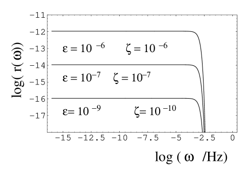
Figure 1: Different spectra are reported for various choices of the parameters. The value of $\xi$ has been fixed to $10^{-12}$ in order to have $m\geq 10^{5}$TeV, as required by electroweak baryogenesis considerations.

In Fig. 2 the shaded area illustrates the region where magnetogenesis is possible.

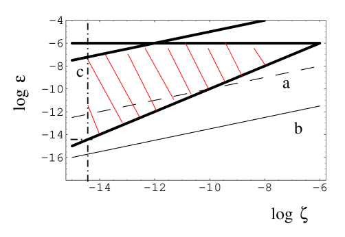
Figure 2: Magnetogenesis requirements are illustrated. The thin line b corresponds to $r_{\rm B}(\omega_{\rm G})\sim 10^{-34}$. The dashed line a corresponds $r_{\rm B}(\omega_{\rm G})\sim 10^{-20}$. The (horizontal) thick line correspond to $\epsilon=10^{-6}$. The (diagonal) thick line corresponds to $\epsilon\sim\zeta$. The thick line c corresponds to the critical density bound which implies $r(\omega)<1$. Since the spectrum is flat (or mildly increasing with the frequency), this bound is also satisfied at large scales. Magnetogenesis is possible when the parameters lie in the shaded area

To be consistent with inflationary production of scalar and tensor fluctuations of the geometry $\epsilon<10^{-6}$ should be imposed. Thus, in Fig. 2 the parameters should all lie below the (horizontal) thick line. Moreover, since $H_{\rm r}<H_{1}$, $\zeta<\epsilon$. Recall that $\zeta>10^{-15}$ in order not to affect the nucleosynthesis epoch [see the dot-dashed line in Fig. 2]. This requirement comes about since $H_{\rm r}>m$ and $\xi\geq 10^{-15}$. In [69] these considerations have been extended to more general evolutions of the gauge coupling.

6 Faraday rotation of CMB

If large scale magnetic fields are truly primordial they should be present prior to the decoupling epoch. Can these fields be “detected” in some way? The effects of large scale magnetic fields possibly present to the decoupling epoch are manifold. Large scale magnetic fields possibly present at the BBN epoch can have an impact on the light nuclei formation. By reversing the argument, the success of BBN can be used in order to bound the magnetic energy density possibly present at the time of formation of light nuclei.

These bounds are qualitatively different from the ones previously quoted and coming, alternatively, from homogeneity [52] and isotropy [53] of the background geometry at the BBN time. As elaborated in slightly different frameworks through the years [82, 83, 84, 85, 86], magnetic fields possibly present at the BBN epoch could have a twofold effect. On one hand they could enhance the rate of reactions (with an effect proportional to $\alpha\rho_{B}$) and, on the other hand they could artificially increase the expansion rate (with an effect proportional to $\rho_{B}$). It turns out that the latter effect is probably the most relevant [85]. In order to prevent the Universe from expanding too fast at the BBN epoch $\rho_{B}<0.27\rho_{\nu}$ where $\rho_{\nu}$ is the energy density contributed by the standard three neutrinos for $T<1$ MeV.

If magnetic fields are present at BBN there are no reasons why they should be absent at the decoupling epoch. Moreover, if quantum mechanical fluctuations of gauge fields are amplified by breaking Weyl invariance, then magnetic fields will be produced over different scales including scales larger than the Mpc.

Large scale magnetic fields present at the decoupling epoch can have various consequences. For instance they can induce fluctuations in the CMB [65, 89], they can distort the Planckian spectrum of CMB [87], they can distort the acoustic peaks of CMB anisotropies [88] and they can also depolarize CMB [90].

The polarization of the CMB represents a very interesting observable which has been extensively investigated in the past both from the theoretical [91] and experimental points of view [92]. Forthcoming satellite missions like PLANCK [93] seem to be able to achieve a level of sensitivity which will enrich decisively our experimental knowledge of the CMB polarization with new direct measurements.

If the background geometry of the universe is homogeneous but not isotropic the CMB is naturally polarized [91]. This phenomenon occurs, for example, in Bianchi-type I models [94]. On the other hand if the background geometry is homogeneous and isotropic (like in the Friedmann-Robertson-Walker [FRW] case) it seems very reasonable that the CMB acquires a small degree of linear polarization provided the radiation field has a non-vanishing quadrupole component at the moment of last scattering [95].

Before decoupling photons, baryons and electrons form a unique fluid which possesses only monopole and dipole moments, but not quadrupole. Needless to say, in a homogeneous and isotropic model of FRW type a possible source of linear polarization for the CMB becomes efficient only at the decoupling and therefore a small degree of linear polarization seems a firmly established theoretical option which will be (hopefully) subjected to direct tests in the near future. The discovery of a linearly polarized CMB could also have a remarkable impact upon other (and related) areas of cosmology. Indeed the linear polarization of the CMB is a very promising laboratory in order to directly probe the speculated existence of a large scale magnetic field (coherent over the horizon size at the decoupling) which might actually rotate (through the Faraday effect [12, 13, 14]) the polarization plane of the CMB.

Consider, for instance, a linearly polarized electromagnetic wave of physical frequency $\omega$ traveling along the $\hat{x}$ direction in a cold plasma of ions and electrons together with a magnetic field ($\overline{B}$) oriented along an arbitrary direction ( which might coincide with $\hat{x}$ in the simplest case). If we let the polarization vector at the origin ($x=y=z=0$, $t=0$) be directed along the $\hat{y}$ axis, after the wave has traveled a length $\Delta x$, the corresponding angular shift ($\Delta\alpha$) in the polarization plane will be :

$$\Delta\alpha=f_{e}\frac{e}{2m}\left(\frac{\omega_{pl}}{\omega}\right)^{2}(\overline{B}\cdot\hat{x})\Delta x$$ (6.1)

(conventions: $\omega_{B}=eB/m$ is the Larmor frequency; $\omega_{pl}=\sqrt{4\pi n_{e}e^{2}/m}$ is the plasma frequency $n_{e}$ is the electron density and $f_{e}$ is the ionization fraction ; we use everywhere natural units $\hbar=c=k_{B}=1$). It is worth mentioning that the previous estimate of the Faraday rotation angle $\Delta\alpha$ holds provided $\omega\gg\omega_{B}$ and $\omega\gg\omega_{pl}$. From Eq. (6.1) by stochastically averaging over all the possible orientations of $\overline{B}$ and by assuming that the last scattering surface is infinitely thin (i.e. that $\Delta xf_{e}n_{e}\simeq\sigma_{T}^{-1}$ where $\sigma_{T}$ is the Thompson cross section) we get an expression connecting the RMS of the rotation angle to the magnitude of $\overline{B}$ at $t\simeq t_{dec}$

$$\langle(\Delta\alpha)^{2}\rangle^{1/2}\simeq 1.6^{0}\left(\frac{B(t_{dec})}{B_{c}}\right)\left(\frac{\omega_{M}}{\omega}\right)^{2},~{}~{}~{}B_{c}=10^{-3}~{}{\rm Gauss},~{}~{}~{}\omega_{M}\simeq 3\times 10^{10}~{}Hz$$ (6.2)

(in the previous equation we implicitly assumed that the frequency of the incident electro-magnetic radiation is centered around the maximum of the CMB). We can easily argue from Eq. (6.2) that if $B(t_{dec})\raise 1.72218pt\hbox{$>$}\kern-6.99997pt\lower 2.6694pt\hbox{$\sim$}B_{c}$ the expected rotation in the polarization plane of the CMB is non negligible. Even if we are not interested, at this level, in a precise estimate of $\Delta\alpha$, we point out that more refined determinations of the expected Faraday rotation signal (for an incident frequency $\omega_{M}\sim 30~{}{\rm GHz}$) were recently carried out [96, 97] leading to a result fairly consistent with (6.1).

Then, the statement is the following. If the CMB is linearly polarized and if a large scale magnetic field is present at the decoupling epoch, then the polarization plane of the CMB can be rotated [90]. The predictions of different models predicting the generation of large scale magnetic fields can then be confronted with the requirements coming from a possible detection of depolarization of the CMB [90].

7 Hypermagnetic fields, EWPT and relic gravitons

If magnetic fields are generated over all physical scales compatible with the plasma dynamics they may have been present even before the BBN epoch, namely at the electroweak epoch. Some of these fields already decayed by today since they are washed out by simultaneous effects of finite magnetic and thermal diffusivities. However, at the electroweak time these fields did not dissipate yet. When we talk about large scale magnetic fields at the electroweak scale we use, as unit, the electroweak time at the epoch of the phase transition.

In this section the we will illustrate the idea that a classical hypermagnetic background can provide an explanation of the possible formation of the BAU giving rise, simultaneously, to stochastic gravitational waves background.

At small temperatures and small densities of different fermionic charges the $SU_{L}(2)\otimes U_{Y}(1)$ is broken down to the $U_{\rm em}(1)$ and the long range fields which can survive in the plasma are the ordinary magnetic fields. However, for sufficiently high temperatures the $SU_{L}(2)\otimes U_{Y}(1)$ is restored and non-screened vector modes correspond to hypermagnetic fields. At the electroweak epoch the typical size of the horizon is of the order of $3$ cm . The typical diffusion scale is of the order of $10^{-9}$ cm. Therefore, over roughly eight orders of magnitude hypermagnetic fields can be present in the plasma without being dissipated [43]. The evolution of hypermagnetic fields can be obtained from the anomalous magnetohydrodynamical (AMHD) equations. The AMHD equations generalize the treatment of plasma effects involving hypermagnetic fields to the case of finite fermionic density[44].

Depending on their topology, hypermagnetic fields can have various consequences [43, 44]. If the hypermagnetic flux lines have a trivial topology they can have an impact on the phase diagram of the electroweak phase transition [104, 105]. If the topology of hypermagnetic fields is non trivial, hypermagnetic knots can be formed [98] and, under specific conditions, the BAU can be generated [99].

A classical hypermagnetic background in the symmetric phase of the EW theory can produce interesting amounts of gravitational radiation in a frequency range between $10^{-4}$ Hz and the kHz. The lower tail falls into the LISA window while the higher tail falls in the VIRGO/LIGO window. For the hypermagnetic background required in order to seed the BAU the amplitude of the obtained GW can be even six orders of magnitude larger than the inflationary predictions. In this context, the mechanism of baryon asymmetry generation is connected with GW production [98, 99].

7.1 Hypermagnetic knots

It is possible to construct hypermagnetic knot configurations with finite energy and helicity which are localized in space and within typical distance scale $L_{s}$. Let us consider in fact the following configuration in spherical coordinates [99]

$${\cal Y}_{r}({\cal R},\theta) = -\frac{2B_{0}}{\pi L_{s}}\frac{\cos{\theta}}{\bigl{[}{\cal R}^{2}+1\bigr{]}^{2}},$$

$${\cal Y}_{\theta}({\cal R},\theta) = \frac{2B_{0}}{\pi L_{s}}\frac{\sin{\theta}}{\bigl{[}{\cal R}^{2}+1\bigr{]}^{2}},$$

$${\cal Y}_{\phi}({\cal R},\theta) = -\frac{2B_{0}}{\pi L_{s}}\frac{n{\cal R}\sin{\theta}}{\bigl{[}{\cal R}^{2}+1\bigr{]}^{2}},$$ (7.1)

where ${\cal R}=r/L_{s}$ is the rescaled radius and $B_{0}$ is some dimensionless amplitude and $n$ is just an integer number whose physical interpretation will become clear in a moment. The hypermagnetic field can be easily computed from the previous expression and it is

$${\cal H}_{r}({\cal R},\theta)=-\frac{4B_{0}}{\pi~{}L_{s}^{2}}\frac{n\cos{\theta}}{\bigl{[}{\cal R}^{2}+1\bigr{]}^{2}},$$

$${\cal H}_{\theta}({\cal R},\theta)=-\frac{4B_{0}}{\pi~{}L_{s}^{2}}\frac{{\cal R}^{2}-1}{\bigl{[}{\cal R}^{2}+1\bigr{]}^{3}}n\sin{\theta},$$

$${\cal H}_{\phi}({\cal R},\theta)=-\frac{8B_{0}}{\pi~{}L_{s}^{2}}\frac{{\cal R}\sin{\theta}}{\bigl{[}{\cal R}^{2}+1\bigr{]}^{3}}.$$ (7.2)

The poloidal and toroidal components of $\vec{{\cal H}}$ can be usefully expressed as $\vec{{\cal H}}_{p}={\cal H}_{r}\vec{e}_{r}+{\cal H}_{\theta}\vec{e}_{\theta}$ and $\vec{\cal H}_{t}={\cal H}_{\phi}\vec{e}_{\phi}$. The Chern-Simons number is finite and it is given by

$$N_{CS}=\frac{g^{\prime 2}}{32\pi^{2}}\int_{V}\vec{{\cal Y}}\cdot\vec{{\cal H}}_{{\cal Y}}d^{3}x=\frac{g^{\prime 2}}{32\pi^{2}}\int_{0}^{\infty}\frac{8nB^{2}_{0}}{\pi^{2}}\frac{{\cal R}^{2}d{\cal R}}{\bigr{[}{\cal R}^{2}+1\bigl{]}^{4}}=\frac{g^{\prime 2}nB^{2}_{0}}{32\pi^{2}}.$$ (7.3)

We can also compute the total helicity of the configuration namely

$$\int_{V}\vec{{\cal H}}_{Y}\cdot\vec{\nabla}\times\vec{{\cal H}}_{Y}d^{3}x=\frac{256~{}B^{2}_{0}~{}n}{\pi L^{2}}\int_{0}^{\infty}\frac{{\cal R}^{2}d{\cal R}}{(1+{\cal R}^{2})^{5}}=\frac{5B^{2}_{0}n}{L_{s}^{2}}.$$ (7.4)

We can compute also the total energy of the field

$$E=\frac{1}{2}\int_{V}d^{3}x|\vec{{\cal H}}_{Y}|^{2}=\frac{B^{2}_{0}}{2~{}L_{s}}(n^{2}+1).$$ (7.5)

and we discover that it is proportional to $n^{2}$. This means that one way of increasing the total energy of the field is to increase the number of knots and twists in the flux lines. We can also have some real space pictures of the core of the knot (i.e. ${\cal R}=r/L_{s}<1$). This type of configurations can be also obtained by projecting a non-Abelian SU(2) (vacuum) gauge field on a fixed electromagnetic direction [100] These configurations have been also studied in [102, 103]. In particular, in [103], the relaxation of HK has been investigated with a technique different from the one employed in [98, 99] but with similar results.

Topologically non-trivial configurations of the hypermagnetic flux lines lead to the formation of hypermagnetic knots (HK) whose decay might seed the Baryon Asymmetry of the Universe (BAU). HK can be dynamically generated provided a topologically trivial (i.e. stochastic) distribution of flux lines is already present in the symmetric phase of the electroweak (EW) theory [98, 99]. In spite of the mechanism generating the HK, their typical size must exceed the diffusivity length scale. In the minimal standard model (MSM) (but not necessarily in its supersymmetric extension) HK are washed out. A classical hypermagnetic background in the symmetric phase of the EW theory can produce interesting amounts of gravitational radiation.

The importance of the topological properties of long range (Abelian) hypercharge magnetic fields has been stressed in the past [106, 107, 108, 109]. In [110] it was argued that if the spectrum of hypermagnetic fields is dominated by parity non-invariant Chern-Simons (CS) condensates, the BAU could be the result of their decay. Most of the mechanisms often invoked for the origin of large scale magnetic fields in the early Universe seem to imply the production of topologically trivial (i.e. stochastic) configurations of magnetic fields [36, 37, 38].

7.2 Hypermagnetic knots and BAU

Suppose that the EW plasma is filled, for $T>T_{c}$ with topologically trivial hypermagnetic fields $\vec{\cal H}_{Y}$, which can be physically pictured as a collection of flux tubes (closed because of the transversality of the field lines) evolving independently without breaking or intersecting with each other. If the field distribution is topologically trivial (i.e. $\langle\vec{\cal H}_{Y}\cdot\vec{\nabla}\times\vec{\cal H}_{Y}\rangle=0$) parity is a good symmetry of the plasma and the field can be completely homogeneous. We name hypermagnetic knots those CS condensates carrying a non vanishing (averaged) hypermagnetic helicity (i.e. $\langle\vec{\cal H}_{Y}\cdot\vec{\nabla}\times\vec{\cal H}_{Y}\rangle\neq 0$). If $\langle\vec{\cal H}_{Y}\cdot\vec{\nabla}\times\vec{\cal H}_{Y}\rangle\neq 0$ parity is broken for scales comparable with the size of the HK, the flux lines are knotted and the field $\vec{{\cal H}}_{Y}$ cannot be completely homogeneous.

In order to seed the BAU a network of HK should be present at high temperatures [43, 44, 110]. In fact for temperatures larger than $T_{c}$ the fermionic number is stored both in HK and in real fermions. For $T<T_{c}$, the HK should release real fermions since the ordinary magnetic fields (present after EW symmetry breaking) do not carry fermionic number. If the EWPT is strongly first order the decay of the HK can offer some seeds for the BAU generation [110]. This last condition can be met in the minimal supersymmetric standard model (MSSM) [111, 112, 113, 114].

Under these hypotheses the integration of the $U(1)_{Y}$ anomaly equation [110] gives the CS number density carried by the HK which is in turn related to the density of baryonic number $n_{B}$ for the case of $n_{f}$ fermionic generations.

$$\frac{n_{B}}{s}(t_{c})=\frac{\alpha^{\prime}}{2\pi\sigma_{c}}\frac{n_{f}}{s}\frac{\langle{\vec{{\cal H}}}_{Y}\cdot\vec{\nabla}\times{\vec{{\cal H}}}_{Y}\rangle}{\Gamma+\Gamma_{{\cal H}}}\frac{M_{0}\Gamma}{T^{2}_{c}},~{}~{}\alpha^{\prime}=\frac{g^{\prime 2}}{4\pi}$$ (7.6)

($g^{\prime}$ is the $U(1)_{Y}$ coupling and $s=(2/45)\pi^{2}N_{eff}T^{3}$ is the entropy density; $N_{eff}$, at $T_{c}$, is $106.75$ in the MSM; $M_{0}=M_{P}/1.66\sqrt{N_{e}ff}\simeq 7.1\times 10^{17}{\rm GeV}$). In Eq. (7.6) $\Gamma$ is the perturbative rate of the right electron chirality flip processes (i.e. scattering of right electrons with the Higgs and gauge bosons and with the top quarks because of their large Yukawa coupling) which are the slowest reactions in the plasma and

$$\Gamma_{{\cal H}}=\frac{783}{22}\frac{\alpha^{\prime 2}}{\sigma_{c}\pi^{2}}\frac{|\vec{{\cal H}}_{Y}|^{2}}{T_{c}^{2}}$$ (7.7)

is the rate of right electron dilution induced by the presence of a hypermagnetic field. In the MSM we have that $\Gamma<\Gamma_{{\cal H}}$ [115] whereas in the MSSM $\Gamma$ can naturally be larger than $\Gamma_{{\cal H}}$. Unfortunately, in the MSM a hypermagnetic field can modify the phase diagram of the phase transition but cannot make the phase transition strongly first order for large masses of the Higgs boson [104]. Therefore, we will concentrate on the case $\Gamma>\Gamma_{\cal H}$ and we will show that in the opposite limit the BAU will be anyway small even if some (presently unknown) mechanism would make the EWPT strongly first order in the MSM.

HK can be dynamically generated [98, 99]. Gauge-invariance and transversality of the magnetic fields suggest that perhaps the only way of producing $\langle\vec{\cal H}_{Y}\cdot\vec{\nabla}\times\vec{\cal H}_{Y}\rangle\neq 0$ is to postulate, a time-dependent interaction between the two (physical) polarizations of the hypercharge field $Y_{\alpha}$. Having defined the Abelian field strength $Y_{\alpha\beta}=\nabla_{[\alpha}Y_{\beta]}$ and its dual $\tilde{Y}_{\alpha\beta}$ such an interaction can be described, in curved space, by the Lagrangian density

$$L_{eff}=\sqrt{-g}\biggl{[}-\frac{1}{4}Y_{\alpha\beta}Y^{\alpha\beta}+c\frac{\psi}{4M}Y_{\alpha\beta}\tilde{Y}^{\alpha\beta}\biggr{]}.$$ (7.8)

where $g_{\mu\nu}$ is the metric tensor and $g$ its determinant, $c$ is the coupling constant and $M$ is a typical scale. This interaction is plausible if the $U(1)_{Y}$ anomaly is coupled, (in the symmetric phase of the EW theory ) to dynamical pseudoscalar particles $\psi$ (like the axial Higgs of the MSSM). Thanks to the presence of pseudoscalar particles, the two polarizations of $\vec{{\cal H}}_{Y}$ evolve in a slightly different way producing, ultimately, inhomogeneous HK.

Suppose that an inflationary phase with $a(\tau)\sim\tau^{-1}$ is continuously matched, at the transition time $\tau_{1}$, to a radiation dominated phase where $a(\tau)\sim\tau$. Consider then a massive pseudoscalar field $\psi$ which oscillates during the last stages of the inflationary evolution with typical amplitude $\psi_{0}\sim M$. As a result of the inflationary evolution $|\vec{\nabla}\psi|\ll\psi^{\prime}$. Consequently, the phase of $\psi$ can get frozen. Provided the pseudoscalar mass $m$ is larger than the inflationary curvature scale $H_{i}\sim{\rm const.}$, the $\psi$ oscillations are converted, at the end of the quasi-de Sitter stage, in a net helicity arising as a result of the different evolution of the two (circularly polarized) vector potentials

$${Y}_{\pm}^{\prime\prime}+\sigma Y^{\prime}_{\pm}+\omega_{\pm}^{2}{Y}_{\pm}=0,~{}~{}\vec{H}_{Y}=\vec{\nabla}\times\vec{Y}$$ (7.9)

$$\omega_{\pm}^{2}=k^{2}\mp k\frac{c}{M}a\dot{\psi}$$ (7.10)

(where we denoted with $\vec{H}_{Y}=a^{2}{\vec{\cal H}}_{Y}$ the curved space fields and with $\sigma=\sigma_{c}a$ the rescaled hyperconductivity; the prime denotes derivation with respect to conformal time $\tau$ whereas the over-dot denotes differentiation with respect to cosmic time $t$).

Since $\omega_{+}\neq\omega_{-}$ the helicity gets amplified according to Eq. (7.9). There are two important points to stress in this context. First of all the plasma effects as well as the finite density effects are important. This means, in practical terms, that the dissipation scales of the problem should be borne in mind. This has not always been done. The second point is related to the first. By treating, consistently, the plasma and finite density effects in the context of AMHD [43, 98, 99], one realizes that the pseudoscalar coupling of $\psi$ together with the coupling of the coupling to the chemical potential are not sufficient in order to seed the BAU unless some hypermagnetic background is already present. In other words the scenario which leads to the generation of the BAU is the following. Correlation in the hypermagnetic fields are generated outside the horizon durin inflation by direct breaking of conformal invariance. An example in this direction has been given in the previous Section. Then hypermagnetic fields re-entering at the electroweak epoch will participate in the dynamics and, in particular, they will feel the effect of the anomalous coupling either to $\psi$ or to the chemical potential. The effect of the anomalous coupling will not be to amplify the hypermagnetic background. The anomalous coupling will make the topology of the hypermagnetic flux lines non-trivial. So the statement is that if conformal invariance is broken and, if hypermagnetic have anomalous couplings, then a BAU $\raise 1.72218pt\hbox{$>$}\kern-6.99997pt\lower 2.6694pt\hbox{$\sim$}10^{-10}$ can be achieved without spoiling the standard cosmological evolution [98, 99]. It is worth mentioning that this type of scenario may be motivated by the low energy string effective action where, by supersymmetry, Kalb-Ramond axions and dilatons are coupled, respectively, to the anomaly and to the gauge kinetic term [116]. It is interesting to notice that, in this scenario, the value of the BAU is determined by various particle physics parameters but also by the ratio of the hypermagnetic energy density over the energy density sitting in radiation during the electroweak epoch, namely, using the language of the previous section [98, 99],

$$\frac{n_{B}}{s}\propto r.$$ (7.11)

In order to get a sizable BAU $r$ should be at least $10^{-3}$ if the anomalous coupling operates during a radiation phase. The value of $r$ coupld be smaller in models where the anomalous coupling is relevant during a low scale inflationary phase [99].

7.3 Hypermagnetic fields and relic gravitons

If a hypermagnetic background is present for $T>T_{c}$, then, as discussed in [117] in the context of ordinary MHD, the energy momentum tensor will acquire a small anisotropic component which will source the evolution equation of the tensor fluctuations $h_{\mu\nu}$ of the metric $g_{\mu\nu}$:

$$h_{ij}^{\prime\prime}+2{\cal H}h_{ij}^{\prime}-\nabla^{2}h_{ij}=-16\pi G\tau^{(T)}_{ij}.$$ (7.12)

where $\tau^{(T)}_{ij}$ is the tensor component of the energy-momentum tensor [117] of the hypermagnetic fields. Suppose now, as assumed in [104] that $|\vec{{\cal H}}|$ has constant amplitude and that it is also homogeneous. Then as argued in [118] we can easily deduce the critical fraction of energy density present today in relic gravitons of EW origin

$$\Omega_{\rm gw}(t_{0})=\frac{\rho_{\rm gw}}{\rho_{c}}\simeq z^{-1}_{{\rm eq}}r^{2},~{}~{}\rho_{c}(T_{c})\simeq N_{\rm eff}T^{4}_{c}$$ (7.13)

($z_{\rm eq}=6000$ is the redshift from the time of matter-radiation, equality to the present time $t_{0}$). Because of the structure of the AMHD equations, stable hypermagnetic fields will be present not only for $\omega_{\rm ew}\sim k_{\rm ew}/a$ but for all the range $\omega_{{\rm ew}}<\omega<\omega_{\sigma}$ where $\omega_{\sigma}$ is the diffusivity frequancy. Let us assume, for instance, that $T_{c}\sim 100$ GeV and $N_{eff}=106.75$. Then, the (present) values of $\omega_{\rm ew}$ is

$$\omega_{\rm ew}(t_{0})\simeq 2.01\times 10^{-7}\biggl{(}\frac{T_{c}}{1{\rm GeV}}\biggr{)}\biggl{(}\frac{N_{\rm eff}}{100}\biggr{)}^{1/6}{\rm Hz}.$$ (7.14)

Thus, $\omega_{\sigma}(t_{0})\sim 10^{8}\omega_{\rm ew}$. Suppose now that $T_{c}\sim 100$ GeV; than we will have that $\omega_{\rm ew}(t_{0})\sim 10^{-5}$ Hz. Suppose now, as assumed in [104], that

$$|\vec{{\cal H}}|/T_{c}^{2}\raise 1.72218pt\hbox{$>$}\kern-6.99997pt\lower 2.6694pt\hbox{$\sim$}0.3.$$ (7.15)

This requirement imposes $r\simeq 0.1$–$0.001$ and, consequently,

$$h_{0}^{2}\Omega_{\rm GW}\simeq 10^{-7}-10^{-8}.$$ (7.16)

Notice that this signal would occurr in a (present) frequency range between $10^{-5}$ and $10^{3}$ Hz. This signal satisfies the presently available phenomenological bounds on the graviton backgrounds of primordial origin. The pulsar timing bound ( which applies for present frequencies $\omega_{P}\sim 10^{-8}$ Hz and implies $h_{0}^{2}\Omega_{\rm GW}\leq 10^{-8}$) is automatically satisfied since our hypermagnetic background is defined for $10^{-5}{\rm Hz}\leq\omega\leq 10^{3}{\rm Hz}$. The large scale bounds would imply $h_{0}^{2}\Omega_{\rm GW}<7\times 10^{-11}$ but a at much lower frequency (i.e. $10^{-18}$ Hz). The signal discussed here is completely absent for frequencies $\omega<\omega_{\rm ew}$. Notice that this signal is clearly distinguishable from other stochastic backgrounds occurring at much higher frequencies (GHz region) like the ones predicted by quintessential inflation [119]. It is equally distinguishable from signals due to pre-big-bang cosmology (mainly in the window of ground based interferometers [120]). The frequency of operation of the interferometric devices (VIRGO/LIGO) is located between few Hz and 10 kHz [120]. The frequency of operation of LISA is well below the Hz. Hence, the background described here lies in the LISA window [98, 99]. In this model the signal can be located both in the LISA window and in the VIRGO/LIGO window due to the hierarchy between the hypermagnetic diffusivity scale and the horizon scale at the phase transition.

8 Concluding remarks

Fifty years after the first seminal speculations on the existence of large scale magnetic fields there are still various dark corners. It is crucial to improve the present evidence on large scale magnetic fields inside clusters. The existence of $\mu$ Gauss magnetic fields inside clusters would be interesting both for magnetogenesis models.The ongoing progress in x-ray astronomy (driven by satellite missions) seems to be rather promising in order to improve our knowledge of the density of charged particles inside the clusters. Even more important would be to obtain observational evidence of magnetic fields right outside the Milky Way. At the moment there is no conclusive evidence of the fact that these fields should be as small as the n Gauss. They can be indeed larger. Another reasonable question often asked discussing large scale magnetic fields concerns the possibility of their primordial origin. In this direction an interesting observable would certainly be the polarization of the CMB. Moreover, large scale magnetic fields present prior to BBN could give rise to an interesting stochastic GW background in the LISA window.

The detection of large scale magnetic fields inside clusters puts pressure on many models of magnetogenesis. Few models predict magnetic fields of reasonable magnitude in this respect. A more complete theoretical understanding of the dynamo mechanism in clusters is certainly needed.

As far as the problem of primordial magnetogenesis is concerned. Few remarks are in order. Causal mechanisms may work at least for the galactic magnetic fields (where the understanding of the dynamo action is more convincing) provided some inverse cascade is realized.As far as inflationary mechanisms are concerned a crucial problem is to find a consistent way in order to break conformal invariance. If gauge couplings are dynamical, conformal invariance may be plausibly broken in the early stages of the inflationary evolution.

ACKNOWLEDGEMENTS

The author wishes to thank M. E. Shaposhnikov for inspiring collaboration. Interesting discussions with M. Laine, H. Kurki-Suonio, E. Sihvola, K. Jedamzik are also acknowledged. Finally the author wishes to thank K. Enqvist, K. Kajantie, K. Kainulainen and M. Ross for the kind invitation to the COSMO-01 meeting.

References

- [1] E. Fermi, Phys. Rev. 75, 1169 (1949).
- [2] H. Alfvén, Arkiv. Mat. F. Astr., o. Fys. 29 B, 2 (1943).
- [3] H. Alfvén, Phys. Rev. 75, 1732 (1949).
- [4] R. D. Richtmyer and E. Teller Phys. Rev. 75, 1729 (1949).
- [5] E. Fermi and Chandrasekar Astrophys. J. 118, 113 (1953).
- [6] K.-T. Kim, P.P. Kronberg, P. D. Dewdney and T. L. Landecker, Astrophys. J. 355, 29 (1990).
- [7] L. Ferretti, D. Dallacasa, G. Giovannini, and A. Tagliani, Astronom. and Astrophys. 302, 680 (1995).
- [8] K.-T. Kim, P. C. Tribble, and P.P. Kronberg, Astrophys. J. 379, 80 (1991).
- [9] O. Goldshmidt and Y. Raphaeli, Astrophys. J. 411, 518 (1993).
- [10] T.E. Clarke, P.P. Kronberg and H. Böhringer astro-ph/0011281.
- [11] H. Böhringer, Rev. Mod. Astron. 8, 295 (1995).
- [12] Ya. B. Zeldovich, A. A. Ruzmaikin, and D.D. Sokoloff, Magnetic Fields in Astrophysics (Gordon and Breach Science, New York, 1983).
- [13] E. N. Parker, Cosmical Magnetic Fields (Clarendon, Oxford, 1979).
- [14] P. P. Kronberg, Rep. Prog. Phys. 57, 325 (1994).
- [15] R. Beck, A. Brandenburg, D. Moss, A. Skhurov, and D. Sokoloff Annu. Rev. Astron. Astrophys. 34 , 155 (1996).
- [16] R. M. Kulsrud, Annu. Rev. Astron. Astrophys. 37, 37 (1999).
- [17] M. Giovannini and M. Shaposhnikov, Phys. Rev. D 62, 103512 (2000).
- [18] A. Vlasov, Zh. Éksp. Teor. Fiz. 8, 291 (1938); J. Phys. 9, 25 (1945).
- [19] L. D. Landau, J. Phys. U.S.S.R. 10, 25 (1945).
- [20] E. M. Lifshitz and L. P. Pitaevskii, Physical Kinetics, (Pergamon Press, Oxford, England, 1980).
- [21] J. Bernstein, Kinetic Theory in the Expanding Universe, (Cambridge University Press, cambridge, England, 1988).
- [22] N. A. Krall and A. W. Trivelpiece, Principles of Plasma Physics, (San Francisco Press, San Francisco 1986).
- [23] D. Biskamp, Non-linear Magnetohydrodynamics (Cambridge University Press, Cambridge, 1994).
- [24] C. P. Dettmann, N. E. Frankel, and V. Kowalenko, Phys. Rev. D 48, 5655 (1993).
- [25] R. M. Gailis, C. P. Dettmann, N. E. Frankel, and V. Kowalenko, Phys. Rev. D 50, 3847 (1994).
- [26] R. M. Gailis, N. E. Frankel, and C. P. Dettmann, Phys. Rev. D 52, 6901 (1995).
- [27] E. N. Parker, Astrophys. J. 122, 293 (1955).
- [28] M. Giovannini, Phys. Rev. D 58, 12407 (1998).
- [29] L. H. Ford, Phys.Rev. D 31, 704 (1985).
- [30] S. A. Colgate, H. Li, and V. Pariev, astro-ph/0012484; S. A. Colgate and H. Li, astro-ph/0001418.
- [31] E. R. Harrison, Phys. Rev. Lett. 30, 188 (1973).
- [32] K. Enqvist, Int.J.Mod.Phys.D 7, 331 (1998).
- [33] D. Grasso and H. Rubinstein, Phys. Rept. 348, 163 (2001).
- [34] A. D. Dolgov, hep-ph/0110293.
- [35] T. Prokopec astro-ph/0106247.
- [36] M. S. Turner and L. M. Widrow, Phys. Rev. D 37, 2734 (1988);T. Vachaspati and A. Vilenkin, Phys.Rev.Lett. 67, 1057 (1991); B. Ratra, Astrophys. J. Lett. 391, L1 (1992); S. Carroll, G. Field and R. Jackiw, Phys. Rev. D 41, 1231 ; W. D. Garretson, G. Field and S. Carroll, Phys. Rev. D 46, 5346 (1992); O. Bertolami and D. Mota, Phys.Lett.B 455, 96 (1999); A. C. davis and K. Dimopoulos, Phys. Rev. D 55, 7398 (1997).
- [37] A. Dolgov and J. Silk, Phys. Rev. D 47, 3144 (1993); A. Dolgov, Phys.Rev.D 48, 2499 (1993).
- [38] K. Enqvist and P. Olesen, Phys. Lett. B 319, 178 (1993); ibid. 329, 195 (1994); T. W. Kibble and A. Vilenkin, Phys. Rev. D 52, 679 (1995); G. Baym, D. Bodeker and L. McLerran, ibid. 53, 662 (1996); J. M. Quashnock, A. Loeb and D. N. Spergel, Astrophys. J. 344, L49 (1989); B. Cheng and A. V. Olinto, Phys. Rev. D 50, 2421 (1994).
- [39] A. Brandenburg, K. Enqvist, and P. Olesen, Phys. Rev. D 54, 1291 (1996).
- [40] A. Brandenburg, K. Enqvist, and P. Olesen, Phys. Lett.B 392, 395 (1997)
- [41] P. Olesen, Phys. Lett. B 398, 321 (1997).
- [42] K. Dimopoulos and A. C. Davis, Phys.Lett. B 390, 87 (1997).
- [43] M. Giovannini and M. Shaposhnikov, Phys. Rev. D 57, 2186 (1998).
- [44] M. Giovannini and M. Shaposhnikov, Phys. Rev. Lett. 80, 22 (1998).
- [45] D. T. Son, Phys. Rev. D 59, 063008 (1999).
- [46] A. Pouquet, U. Frish, and J. Léorat, J. Fluid Mech. 77, 321 (1976); J. Léorat, A. Pouquet, and U. Frish ibid. 104, 419 (1981).
- [47] M. Christensson and M. Hindmarsh, Phys.Rev.D 60, 063001 (1999); M. Hindmarsh, these proceedings.
- [48] A. Berera and D. Hochberg, cond-mat/0103447.
- [49] D. N. Schramm, R. V. Wagoner, Ann. Rev. Nucl. Part. Sci. 27, 37 (1977).
- [50] S. Sarkar, Rept. Prog. Phys. 59, 1493 (1996).
- [51] V. A. Rubakov and M. E. Shaposhnikov Usp.Fiz.Nauk 166,493 (1996) [Phys.Usp. 39, 461 (1996)].
- [52] K. Jedamzik and G. M. Fuller, Astrophys. J. 423, 33 (1994); H. Kurki-Suonio K. Jedamzik and G.J. Mathews, Astrophys. J. 479, 31 (1997); K. Kainulainen, H. Kurki-Suonio, E. Sihvola, Phys.Rev.D 59 083505 (1999).
- [53] K. S. Thorne, Astrophys. J. 148, 51 (1967); S. W. Hawking and R. J. Tayler, Nature 309, 1278 (1966); J. D. Barrow, Mon. Not. R. Astron. Soc. 175, 359 (1976).
- [54] G. Steigman, Ann. Rev. Astron. Astroph. 14, 339 (1976).
- [55] H. Kurki-Suonio and E. Sihvola, Phys. Rev. Lett. 84 3756 (2000); Phys.Rev.D 62, 103508 (2000).
- [56] J. B. Rehm and K. Jedamzik, Phys.Rev.Lett. 81, 3307 (1998); Phys.Rev.D 64, 023510 (2001)
- [57] J. D. Barrow, Phys. Rev. D 35, 1805 (1987).
- [58] E. W. Kolb, M. J. Perry, and T.P. Walker, Phys. Rev. D 33, 869 (1986); F. S. Accetta, L. M. Krauss, and P. Romanelli, Phys. Lett. B 248, 146 (1990).
- [59] T. Appelquist, A. Chodos, and P. G. O. Freund, Modern Kaluza Klein Theories (Addison-Wesley, Redwood City, CA, 1987).
- [60] M. B. Green, J. H. Schwartz, and E. Witten, Superstring Theory (Cambridge University Press, Cambridge, England, 1987).
- [61] J.K. Webb, M.T. Murphy, V.V. Flambaum, V.A. Dzuba, J.D. Barrow, C.W. Churchill, J.X. Prochaska, and A.M. Wolfe, Phys. Rev Lett. 87, 091301 (2001).
- [62] M.T. Murphy, J.K. Webb, V.V. Flambaum, V.A. Dzuba, C.W. Churchill, J.X. Prochaska, J.D. Barrow, and A.M. Wolfe, Mon. Not. Roy. Astron. Soc. 327, 1208 (2001).
- [63] J. K. Webb, V. V. Flambaum, C. W. Churchill, M. J. Drinkwater, and J. D. Barrow, Phys. Rev. Lett. 82, 884 (1999).
- [64] M. Giovannini, Phys.Rev.D 55 595 (1997).
- [65] M. Gasperini, M. Giovannini and G. Veneziano, Phys. Rev. Lett. 75, 3796 (1995); Phys. Rev. D 52, 6651 (1995); M. Giovannini, Phys.Rev.D 59, 123518 (1999).
- [66] M. Giovannini, Phys.Rev.D 56, 631 (1997).
- [67] M. Giovannini, Phys.Rev.D 62 123505 (2000).
- [68] M. Giovannini, Phys.Rev. D 64, 061301 (2001);
- [69] M. Giovannini, hep-ph/0104214.
- [70] P. A. M. Dirac, Nature 139, 323 (1937); Proc. R. Soc. London A 165, 199 (1938).
- [71] P. Jordan, Z. Phys. 157, 112 (1959).
- [72] E. Teller, Phys. Rev. 73 , 801 (1948).
- [73] J. D. Bekenstein, Phys. Rev. D 25, 1527 (1982).
- [74] Smith et al., Phys. Rev. D 61, 022001 (2000); J. C. Long et al., hep-ph/0009062.
- [75] C. D. Hoyle et al., Phys. Rev. Lett. 86, 1418 (2001).
- [76] G. German and G. G. Ross, Phys. Lett. B 172 305 (1986).
- [77] A. S. Goncharov, A. D. Linde and M. Vysotsky, Phys. Lett. B 147 279 (1993).
- [78] M. Gasperini, Phys. Lett. B 327, 214 (1994).
- [79] V. A. Kuzmin, V. A. Rubakov and M. E. Shaposhnikov, Phys. Lett. B 155, 36 (1985); V. A. Robakov and M. E. Shaposhnikov, Phys. Usp. 39, 461 (1996) [Usp.Fiz.Nauk 166, 493 (1996)].
- [80] M. E. Shaposhnikov, JETP Lett. 44, 465 (1986).
- [81] M. Giovannini and M. Shaposhnikov, Phys. Rev. D 62, 103512 (2000).
- [82] G. Greenstein, Nature 223, 938 (1969).
- [83] J. J. Matese and R. F. O’ Connel, Astrophys. J. 160, 451 (1970).
- [84] B. Cheng, D. N. Schramm and J. Truran, Phys. Rev. D 45, 5006 (1994); B. Cheng, A. Olinto, D. N. Schramm and J. Truran, Phys. Rev. D 54, 4174 (1996).
- [85] P. Kernan, G. Starkman and T. Vachaspati, Phys. Rev. D 54, 7207 (1996).
- [86] D. Grasso and H. Rubinstein, Astropart. Phys. 3, 95 (1995) and Phys. Lett. B 379, 73 (1996).
- [87] K. Jedamzik, V. Katalinic, and A. V. Olinto, Phys. Rev. Lett. 85 700, (2000).
- [88] J. Adams, U. H. Danielsson, D. Grasso, and Hector Rubinstein, Phys.Lett.B 388, 253 (1996).
- [89] R. Durrer, M. Gasperini, M. Sakellariadou, and G. Veneziano, Phys. Rev.D 59, 043511 (1999).
- [90] M. Giovannini, Phys. Rev. D 56, 3198 (1997).
- [91] M. Rees, Astrophys. J. 153, L1 (1968).
- [92] P. M. Lubin and G. F. Smoot, Astrophys. J. 245, 1 (1981); P. M. Lubin, P. Melese and G. F. Smoot, Astrophys. J. Lett. 273, L51 (1983).
- [93] M. Bersanelli et. al. Esa D/Sci(96)3; home page of the Cambridge Planck Analysis Center (CPAC) [http://www.mrao.cam.ac.uk/projects/cpac/].
- [94] E. Milaneschi and R. Fabbri, Astron. Astrophys. 151, 7 (1985).
- [95] D. Coulson, R. Crittenden and N. G. Turok, Phys. Rev. D 52, 5402 (1995); Phys. Rev. Lett. 73, 2390 (1994).
- [96] A. Kosowsky and A. Loeb, Astrophys. J 461, 1 (1996).
- [97] D. Harari, J. Hayward and M. Zaldarriaga, Phys. Rev. D 55 (1997).
- [98] M.Giovannini, Phys.Rev.D 61, 063502 (2000).
- [99] M. Giovannini, Phys.Rev.D 61, 063004 (2000).
- [100] R. Jackiw and S.-Y. Pi, Phys.Rev. D 61, 105015 (2000).
- [101] R. Jackiw, V.P. Nair, S-Y. Pi, Phys.Rev.D 62, 085018 (2000).
- [102] C. Adam, B. Muratori, and C. Nash Phys.Rev.D 61, 105018 (2000).
- [103] C. Adam, B. Muratori, and C. Nash, Phys.Rev.D 62, 105027 (2000).
- [104] K. Kajantie,M. Laine, J. Peisa, K. Rummukainen, M. Shaposhnikov, Nucl.Phys.B 544, 357 (1999).
- [105] P. Elmfors, K. Enqvist, and K. Kainulainen, Phys.Lett.B 440 269, (1998).
- [106] A. Vilenkin, Phys. Rev. D 22, 3067 (1980).
- [107] V. Rubakov and A. Tavkhelidze, Phys. Lett. B 165, 109 (1985).
- [108] V. Rubakov, Prog. Theor. Phys. 75, 366 (1986).
- [109] A. N. Redlich and L. C. R. Wijewardhana, Phys. Rev. Lett. 54, 970 (1984).
- [110] M. E. Shaposhnikov, Nucl. Phys. B 287, 757 (1987);ibid. 299, 797 (1988).
- [111] K. Kajantie, M. Laine, K. Rummukainen and M. Shaposhnikov, Nucl. Phys. B 495, 413 (1997).
- [112] M. Carena, M. Quiros and C. Wagner, Phys. Lett. B 380, 81 (1996).
- [113] M. Laine Nucl. Phys. B 481, 43 (1996).
- [114] J. Cline and K. Kainulainen, Nucl. Phys. B 482, 73 (1996).
- [115] B. Campbell, S. Davidson, J. Ellis and K. Olive, Phys. Lett. 297B , 118, (1992); L. E. Ibanez and F. Quevedo, Phys. Lett., B283, 261, 1992; J. M. Cline, K. Kainulainen and K. A. Olive, Phys. Rev. Lett. 71, 2372 (1993); Phys. Rev. D 49, 6394 (1993).
- [116] M. Giovannini, Phys. Rev.D 59, 063503 (1999).
- [117] M. Giovannini, Phys. Rev.D 58, 124027 (1998).
- [118] D. Deryagin, D. Grigoriev, V. Rubakov and M. Sazhin, Mod. Phys. Lett. A 11, 593 (1986).
- [119] M. Giovannini, Phys.Rev. D 60, 123511 (1999).
- [120] D. Babusci and M. Giovannini, Int.J.Mod.Phys. D 10, 477 (2001); Class. Quant. Grav. 17, 2621 (2000).