Chemical equilibration of U(1) charged particles in a thermal environment

Abstract

We discuss chemical equilibration of particles carrying non-vanishing quantum numbers related with U(1) internal symmetry. We construct the transport equation for the time evolution of particle multiplicities and their probability functions. The solution of these equations is obtained in different limiting cases. It is argued that a U(1) charged particles, dependent on thermal conditions inside a fireball, approaches different equilibrium limits. The differences between kinetics of abundantly and rarely produced particles are explained.

I introduction

One of the crucial questions being addressed in the context of heavy ion collisions is the equilibration of the high density QCD medium created during these collisions [1, 2, 3, 4]. This question has been considered on different levels: by analysing physical conditions required for a perturbative QCD medium to reach equilibrium [5] or by studying the level of particle equilibration in the final state [6, 7]. From the theoretical point of view to discuss equilibration one needs to formulate the kinetic equation for particle production and evolution. In the partonic medium this requires, in general, the formulation of a transport equation involving colour degrees of freedom and a non-abelian structure of QCD dynamics [8, 9, 10]. In the hadronic medium, on the other hand, one needs to account for the charge conservations related with U(1) internal symmetry [11, 12, 13].

In this article we will discuss the formulation of kinetic equations for U(1) charged particles produced in a thermal environment. We will indicate the importance of the conservation laws in the time evolution and chemical equilibration of particle multiplicities and their probability distributions. In particular we will argue that the constraints imposed by U(1) charge conservation are of crucial importance for rarely produced charged particle species.

II Kinetic master equation for probabilities with U(1) symmetry constraints

To study equilibration in a hadronic medium one introduces a kinetic model that takes into account the production and annihilation of particle–antiparticle pairs $c\bar{c}$ carrying U(1) quantum numbers. It is also assumed that particles $c$ are produced according to a binary process $ab\to c\bar{c}$ and that all particle momentum distributions are thermal and described by Boltzmann statistics. The U(1) charge neutral particles $a$ and $b$ are constituents of a thermal fireball of temperature $T$ and volume $V$. We will consider the time evolution and equilibration of particles $c$ inside a thermal fireball, taking into account the constraints imposed by U(1) symmetry. First we formulate a general master equation for the probability distribution of particle multiplicity in the medium with vanishing net charge and consider its properties and solutions. We will then discuss two limiting cases of abundant and rare particle production. Finally the rate equation will be extended to the situation where there is a net U(1) charge in the thermal fireball.

A Rate equation for particle multiplicity distribution

Consider $P_{N_{c}}(t)$ as the probability to find $N_{c}$ particles $c$, where $0\leq N_{c}\leq\infty$. This probability will obviously change in time owing to production $ab\to c\bar{c}$ and absorption $c\bar{c}\to ab$ processes. The probability $P_{N_{c}}$ tends to increase in time, following the transition from $N_{c}-1$ and $N_{c}+1$ states to the $N_{c}$ state. It also tends to decrease since the state $N_{c}$ makes transitions to $N_{c}+1$ and $N_{c}-1$ (see Fig. 1). The transition probability per unit time from $N_{c}+1\to N_{c}$ is given by the product of the probability $L/V$ that the single reaction $c\bar{c}\to ab$ takes place multiplied by the number of possible reactions which is, $(N_{c}+1)(N_{\bar{c}}+1)$. In the case when the U(1) charge carried by particles $c$ and $\bar{c}$ is exactly and locally conserved, that is if $N_{c}+N_{\bar{c}}=0$; then this number is just $(N_{c}+1)^{2}$. Similarly the transition probability from $N_{c}\to N_{c}+1$ is described by $G\langle N_{a}\rangle\langle N_{b}\rangle/V$, where one assumes that particles $a$ and $b$ are not correlated and their multiplicity is governed by the thermal averages. One also assumes that the multiplicity of $a$ and $b$ is not affected by the $ab\to c\bar{c}$ process.

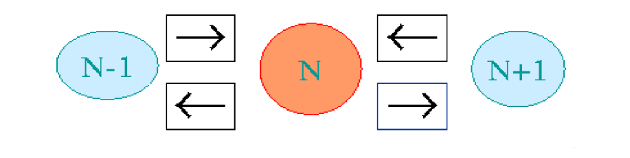
FIG. 1.: Schematic view of the master equation for the probability $P_{N}(\tau)$ due to $ab\to c\bar{c}$ and the inverse process.

The master equation for the time evolution of the probability $P_{N_{c}}(\tau)$ can be written in the following form [11]:

$$\frac{dP_{N_{c}}}{d\tau} = {G\over V}\langle N_{a}\rangle\langle N_{b}\rangle P_{N_{c}-1}+\frac{L}{V}(N_{c}+1)^{2}P_{N_{c}+1}$$ (1)

$$- {G\over V}\langle N_{a}\rangle\langle N_{b}\rangle P_{N_{c}}~{}~{}~{}-\frac{L}{V}N_{c}^{2}P_{N_{c}}.$$ (2)

The first two terms in Eq. (2) describe the increase of $P_{N_{c}}(\tau)$ due to the transition from $N_{c}-1$ and $N_{c}+1$ to the $N_{c}$ state. The last two terms, on the other hand, represent the decrease of the probability function due to the transition from $N_{c}$ to $N_{c}+1$ and $N_{c}-1$ states respectively.

Multiplying the above equation by $N_{c}$ and summing over $N_{c}$, one obtains the general kinetic equation for the time evolution of the average number $\langle N_{c}\rangle\equiv\sum_{N_{c}=0}^{\infty}N_{c}P_{N_{c}}(\tau)$ of particles $c$ in a system. This equation reads:

$$\frac{d\langle N_{c}\rangle}{d\tau}={G\over V}\langle N_{a}\rangle\langle N_{b}\rangle-\frac{L}{V}\langle N_{c}^{2}\rangle.$$ (3)

The above equation cannot be obviously solved analytically as it connects particle multiplicity $\langle N_{c}\rangle$ with its second moments $\langle N_{c}^{2}\rangle$. However, the solution can be obtained in two limiting situations: i) for abundant production of $c$ particles, that is when $\langle N_{c}\rangle\gg 1$ or ii) in the opposite limit of rare particle production corresponding to $\langle N_{c}\rangle\ll 1$. Indeed, since

$${\langle N_{c}^{2}\rangle}=\langle N_{c}\rangle^{2}+\langle\delta N_{c}^{2}\rangle,$$ (4)

where $\langle\delta N_{c}^{2}\rangle$ represents the fluctuations of the number of particles $c$, one can make the following approximations:

i) for $\langle N_{c}\rangle\gg 1$ one has, $\langle N_{c}^{2}\rangle\approx\langle N_{c}\rangle^{2},$ and Eq. (2) obviously reduces to the well known form [14]:

$$\frac{d\langle N_{c}\rangle}{d\tau}\approx{G\over V}\langle N_{a}\rangle\langle N_{b}\rangle-\frac{L}{V}\langle N_{c}\rangle^{2};$$ (5)

however, for rare production, particles $c$ and $\bar{c}$ are strongly correlated; then,

ii) $\langle N_{c}\rangle\ll 1$ and $\langle N_{c}^{2}\rangle\approx\langle N_{c}\rangle$; consequently Eq. (2) takes the form:

$$\frac{d\langle N_{c}\rangle}{d\tau}\approx{G\over V}\langle N_{a}\rangle\langle N_{b}\rangle-\frac{L}{V}\langle N_{c}\rangle,$$ (6)

where the absorption term depends only linearly, instead of quadratically, on the particle multiplicity.

From the above discussion it is thus clear that depending on the thermal conditions of the system (that is its volume and the value of the temperature) we are getting different results for the equilibrium solution and the time evolution of the number of produced particles $c$. This is very transparent when solving the rate equations (4) and (5).

In the limit when $\langle N_{c}\rangle\gg 1$, the standard Eq. (5) is valid and has the well known solution:

$$\langle N_{c}\rangle(\tau)=\langle N_{c}\rangle_{\rm eq}\tanh\left(\tau/\tau_{0}\right),$$ (7)

where the equilibrium value $\langle N_{c}\rangle_{\rm eq}$ of the number of particles $c$ and the relaxation time constant $\tau_{0}$ are given by:

$$\langle N_{c}\rangle_{\rm eq}=\sqrt{\epsilon}~{}~{},~{}~{}\tau_{0}=\frac{V}{L\sqrt{\epsilon}},$$ (8)

respectively, with $\epsilon\equiv G\langle N_{a}\rangle\langle N_{a}\rangle/L$.

In the particular case when the particle momentum distribution is thermal, the gain ($G$) and loss ($L$) terms are just the thermal averages of the absorption and production cross sections with [11]

$$\frac{G}{L}=\frac{\langle N_{c}\rangle_{\rm eq}\langle N_{\bar{c}}\rangle_{\rm eq}}{\langle N_{a}\rangle_{\rm eq}\langle N_{b}\rangle_{\rm eq}},$$ (9)

where we have employed the detailed balance relation between production $\sigma_{ab}$ and absorbtion $\sigma_{c\bar{c}}$ cross section for $ab\to c\bar{c}$ processes.

Assuming a Boltzmann particle momentum distribution, the equilibrium average number of particles $k$ is obtained after momentum integration as:

$$\langle N_{k}\rangle_{\rm eq}={{d_{k}}\over{2\pi^{2}}}VTm_{k}^{2}K_{2}(m_{k}/T),$$ (10)

where $d_{k}$’s denote spin–isospin degeneracy factors, $m_{k}$ the particle mass, and $K_{2}$ is the modified Bessel function.

This is a well known result for the average number of particles in the Grand Canonical (GC) ensemble with respect to U(1) charge conservation. The chemical potential, which is usually present in the GC ensemble, vanishes in our case, because of the requirement of U(1) charge neutrality of a system. Thus, the solution (5) results in the expected value for the equilibrium limit in GC formalism where the charge is conserved on the average.

In the opposite limit, where $\langle N_{c}\rangle\ll 1$, the time evolution of particle abundance is described by Eq. (5), which has the following solution:

$$\langle N_{c}\rangle^{\rm C}(\tau)=\langle N_{c}\rangle_{\rm eq}^{\rm C}\left(1-e^{-\tau/\tau_{0}^{\rm C}}\right),$$ (11)

with the equilibrium value and relaxation time given by

$$\langle N_{c}\rangle_{\rm eq}^{\rm C}=\epsilon,~{}\tau_{0}^{\rm C}=\frac{V}{L}.$$ (12)

The above result is the asymptotic limit of the canonical C formulation of conservation laws [11]. Here the charge related with U(1) symmetry is exactly and locally conserved, contrary to the GC formulation where this conservation is only valid on the average.

Comparing Eq. (8) with Eq. (12), we first find that, for $\langle N_{c}\rangle\ll 1$, the equilibrium value in the canonical formulation is far smaller than what is expected from the grand canonical result as

$$\langle N_{c}\rangle_{\rm eq}^{\rm C}={\langle N_{c}\rangle_{\rm eq}}^{2}\ll{\langle N_{c}\rangle_{\rm eq}}.$$ (13)

Secondly, we can conclude that the relaxation time for a canonical system is far shorter than what is expected from the grand canonical value as

$$\tau_{0}^{\rm C}=\tau_{0}\langle N_{c}\rangle_{\rm eq}\ll\tau_{0},$$ (14)

since in the limit $\bf(ii)$ the equilibrium value $\langle N_{c}\rangle_{\rm eq}\ll 1$.

The above discussion shows the importance of the canonical description of quantum number conservation if the U(1) charged particle multiplicity is small. We also see that the volume dependence differs in the two cases. The particle density in the GC limit is $V$-independent whereas, in the opposite case, the density scales linearly with $V$.

We note that $\bf(i)$ and $\bf(ii)$ limits are essentially determined by the size of $\langle\delta N_{c}^{2}\rangle$, the fluctuation of the number of particles $c$. The grand canonical results correspond to small fluctuations, i.e. $\langle\delta N_{c}^{2}\rangle/\langle N_{c}\rangle^{2}\ll 1$, while the canonical description is relevant if the fluctuations are large, i.e. $\langle\delta N_{c}^{2}\rangle/\langle N_{c}\rangle^{2}\gg 1$.

III Master equation - general solution

In the previous section, we formulated a general master equation (1) for the probability to find the number of U(1) charged particles being produced by the binary $ab\to c\bar{c}$ process. The approximate solutions of Eq. (1) were considered in two limiting cases. For a large number of produced particles carrying U(1) charge, the time evolution and the equilibrium limit of Eq. (1) correspond to the GC result. We have also indicated the difference between GC and asymptotic C results on the level of rate equations for particle multiplicity. This difference is particularly transparent when comparing master equations for probabilities.

A Master equation for abundant U(1) charged particle production

For abundantly produced particles $c$ and $\bar{c}$ through $ab\to c\bar{c}$, process we do not need to worry about strong particle correlations due to U(1) charge conservation. This also means that instead of imposing U(1) charge neutrality conditions through $N_{c}-N_{\bar{c}}=0$, one assumes conservation on the average, that is $\langle N_{c}\rangle-\langle N_{\bar{c}}\rangle=0$. In this case the master equation (1) can be simplified.

In the derivation of Eq. (1) the absorption terms proportional to $L$ were obtained by constraining the U(1) charge conservation to be local and exact. For the conservation on the average, the transition probability from $N_{c}$ to the $(N_{c}-1)$ state is no longer proportional to $(L/V)N_{c}^{2}$ but rather to $(L/V)N_{c}\langle N_{\bar{c}}\rangle$, since the exact conservation condition $N_{c}=N_{\bar{c}}$ is no longer valid and the number of $\bar{c}$ particles can only be determined by its average value. In the GC limit, the master equation for the time evolution of the probability $P_{N_{c}}(\tau)$ takes the following form:

$$\frac{dP_{N_{c}}}{d\tau} = {G\over V}\langle N_{a}\rangle\langle N_{b}\rangle P_{N_{c}-1}+\frac{L}{V}(N_{c}+1)\langle N_{\bar{c}}\rangle P_{N_{c}+1}$$ (15)

$$- {G\over V}\langle N_{a}\rangle\langle N_{b}\rangle P_{N_{c}}~{}~{}~{}-\frac{L}{V}N_{c}\langle N_{\bar{c}}\rangle P_{N_{c}}.$$ (16)

Multiplying the above equation by $N_{c}$, summing over $N_{c}$ and using the condition that $\langle N_{c}\rangle=\langle N_{\bar{c}}\rangle$, one recovers Eq. (4), the rate equation for $\langle N_{c}\rangle$ in the GC ensemble. The above equation is thus indeed the general master equation for the probability function in the GC limit. Comparing this equation with the more general Eq. (1), one can see that the main difference is contained in the absorption terms, which are linear instead of quadratic in particle number.

Equation (14) can be solved exactly. Indeed, introducing the generating function $g(x,\tau)$ for $P_{N_{c}}$,

$$g(x,{\tau})=\sum_{N_{c}=0}^{\infty}x^{N_{c}}P_{N_{c}}(\tau),$$ (17)

the iterative equation (14) for probability can be converted into a differential equation for the generating function:

$$\frac{\partial g(x,\tau)}{\partial\tau}={{L}\over V}\sqrt{\epsilon}(1-x)[g^{\prime}-{\sqrt{\epsilon}}g],$$ (18)

with the general solution [13]:

$$g(x,\tau)=g_{0}(1-xe^{-\tilde{\tau}})e^{\sqrt{\epsilon}(1-x)(e^{-\tilde{\tau}}-1)},$$ (19)

where $g^{\prime}\equiv\partial g/\partial x$, $\tilde{\tau}=(L\sqrt{\epsilon}/V)\tau$ and $\sqrt{\epsilon}=\langle N_{c}\rangle_{eq}$ given by Eq. (9).

One can readily find the equilibrium solution to the above equation. Taking the limit $\tau=\infty$ in Eq. (17) leads to

$$g_{\rm eq}(x)=e^{-\sqrt{\epsilon}(1-x)},$$ (20)

with the corresponding equilibrium multiplicity distribution:

$$P_{N_{c},{\rm eq}}=\frac{(\sqrt{\epsilon})^{N_{c}}}{{N_{c}}!}e^{-\sqrt{\epsilon}}.$$ (21)

This is a Poisson distribution with averaged multiplicity $\sqrt{\epsilon}$.

B Equilibrium solution - general case

The master equation (14), describing the evolution of the probability function in the GC limit, could be solved exactly. The general equation (1), however, because the quadratic dependence of the absorption term, can only be solved numerically. Nevertheless the equilibrium result for particle multiplicity can be given.

Converting Eq. (1) for $P_{N_{c}}$’s into a partial differential equation for the generating function

$$g(x,\tau)=\sum_{N_{c}=0}^{\infty}x^{N_{c}}P_{N_{c}}(\tau).$$ (22)

one finds [11]

$$\frac{\partial g(x,\tau)}{\partial\tau}=\frac{L}{V}(1-x)\left(xg^{\prime\prime}+g^{\prime}-\epsilon g\right).$$ (23)

The equilibrium solution $g_{\rm eq}(x)$ thus obeys the following equation:

$$xg_{\rm eq}^{\prime\prime}+g_{\rm eq}^{\prime}-\epsilon g_{\rm eq}=0.$$ (24)

By a substitution of variables ($x=y^{2}/4/\epsilon$), this equation is reduced to the Bessel equation, with the following solution:

$$g_{\rm eq}(x)=\frac{1}{I_{0}(2\sqrt{\epsilon})}I_{0}(2\sqrt{\epsilon x}),$$ (25)

where the normalization is fixed by $g(1)=\sum P_{N_{c}}=1$.

The equilibrium value for the probability function $P_{N_{c}}$ is now expressed from Eqs. (20–23) as:

$$P_{N_{c},\rm eq}=\frac{\epsilon^{N_{c}}}{I_{0}(2\sqrt{\epsilon})(N_{c}!)^{2}}.$$ (26)

We note that the equilibrium distribution of the particle multiplicity in not a Poissonian. This fact was first indicated in equilibrium studies in [15]. In our case this is a direct consequence of the quadratic dependence on the multiplicity in the loss terms of the master equation (1). A Poisson distribution is obtained from Eq. (24) if $\sqrt{\epsilon}\gg 1$, that is for large particle multiplicity. In this case the C ensemble coincides with the GC approximation.

The result for the equilibrium average number of particles $c$ can be obtained as:

$$\langle N_{c}\rangle_{\rm eq}=g^{\prime}(1)=\sqrt{\epsilon}\frac{I_{1}(2\sqrt{\epsilon})}{I_{0}(2\sqrt{\epsilon})}.$$ (27)

The equilibrium solution presented above coincides with the expected result for the particle multiplicity in the canonical ensemble with respect to U(1) charge conservation [16]. Thus, the rate equation formulated in Eq. (1) is valid for any arbitrary value of $\langle N_{c}\rangle$ and obviously reproduces the standard grand canonical result for large $\langle N_{c}\rangle$. We can study the chemical equilibration of U(1) charged particles following Eq. (1) independently from the thermal conditions in a system.

C Master equation for net U(1) charge in thermal environment

So far, constructing the evolution equation for probabilities, we have assumed that there is no net U(1) charge in a system. In the application of the statistical approach to particle production in heavy ion collisions, the above assumption is only justified when the initial state is U(1) charge neutral and when considering particle yields in full phase space. However, because of experimental limitations, one often deals with data in restricted kinematical windows. Here the overall U(1) charge is no longer zero and a generalization of the above master equation is required.

In the following we construct the evolution equation for $P_{N_{c}}^{S}(t)$ in a thermal medium assuming that its net U(1) charge $S$ is non–vanishing. The presence of the net charge requires a modification of absorption terms in Eq. (1). The transition probability per unit time from the $N_{c}$ to the $N_{c}-1$ state was proportional to $(L/V)N_{c}N_{\bar{c}}$. Given an over all net charge $S$ the exact U(1) charge conservation implies that $N_{c}-N_{\bar{c}}=S$. The transition probability from $N_{c}$ to $N_{c}-1$ due to pair annihilation is thus $(L/V)N_{c}(N_{c}-S)$. Following the same procedure as in Eq. (1) one can formulate the following master equation for the probability $P_{N_{c}}^{S}(t)$ to find $N_{c}$ particles $c$ in a thermal medium with a net charge $S$:

$$\frac{dP_{N_{c}}^{S}}{d\tau} = {G\over V}\langle N_{a}\rangle\langle N_{b}\rangle P_{N_{c}-1}^{S}+\frac{L}{V}(N_{c}+1)(N_{c}+1-S)P_{N_{c}+1}^{S}$$ (28)

$$- {G\over V}\langle N_{a}\rangle\langle N_{b}\rangle P_{N_{c}}^{S}~{}~{}~{}-\frac{L}{V}N_{c}(N_{c}-S)P_{N_{c}}^{S},$$ (29)

which obviously reduces to Eq. (2) for $S=0$.

To get the equilibrium solution for the probability and multiplicity, we again convert the above equation to the differential form for the generating function $g^{S}(x,\tau)=\sum_{N_{c}=0}^{\infty}x^{N_{c}}P_{N_{c}}^{S}(\tau)$:

$$\frac{\partial g^{S}(x,\tau)}{\partial\tau}=\frac{L}{V}(1-x)\left(xg_{S}^{\prime\prime}+g_{S}^{\prime}(1-S)-\epsilon g_{S}\right).$$ (30)

In equilibrium, ${\partial g^{S}(x,\tau)}{\partial\tau}=0$ and the solution for $g^{S}_{\rm eq}$ can be found as follows:

$$g_{\rm eq}(x)=\frac{x^{S/2}}{I_{S}(2\sqrt{\epsilon})}I_{S}(2\sqrt{\epsilon x}),$$ (31)

where the normalization is fixed by $g(1)=\sum P_{n}=1$.

The master equation for the probability to find $N_{\bar{c}}$ antiparticles $\bar{c}$, its corresponding differential form and the equilibrium solution for the generating function can be obtained by replacing $S\to-S$ in Eqs. (26-28)

The result for the equilibrium average number of particles $\langle N_{c}\rangle_{\rm eq}$ and antiparticles $\langle N_{\bar{c}}\rangle_{\rm eq}$ is obtained from the generating function using the relation: $\langle N_{c}\rangle_{\rm eq}=g^{\prime}(1)$. The final expressions read:

$$\langle N_{c}\rangle_{\rm eq}=\sqrt{\epsilon}\frac{I_{S-1}(2\sqrt{\epsilon})}{I_{S}(2\sqrt{\epsilon})}~{}~{},~{}~{}\langle N_{\bar{c}}\rangle_{\rm eq}=\sqrt{\epsilon}\frac{I_{S+1}(2\sqrt{\epsilon})}{I_{S}(2\sqrt{\epsilon})}.$$ (32)

The strangeness conservation is explicitly seen by taking the difference of these equations, which yields, the net value of the U(1) charge $S$.

The results of Eq. (32) were previously derived from the equilibrium partition function by using the projection method [16]. The master equation derived here allows a study of the time evolution of particle production in a thermal medium and the approach towards chemical equilibrium. This equation explicitly accounts for U(1) charge conservation for both strongly correlated and uncorrelated particles.

The results presented here can be extended to the more general case where there are different particle species carrying the U(1) charge being produced in a thermal environment [12].

IV Concluding remarks

We have discussed the kinetics and chemical equilibration of particles carrying quantum numbers related with U(1) symmetry. Our analysis was restricted to the particular case of one kind of particle and antiparticle being produced by the binary process. However, this example is of physics interest as it can be applied to the study of such problems as the equilibration of heavy quarks in QCD plasma due to gluon–gluon fusion or strangeness and baryon production due to baryon–baryon and meson–meson interactions. The last process is of relevance in the application of statistical models to the description of particle production in low energy heavy ion collisions [11, 12, 16, 17]. We have discussed the procedure that allows the construction of the rate for time evolution of particle multiplicity and its probability distribution. Our result is quite general and applicable, as well as for abundantly and rarely produced U(1) charged particles. We have indicated the important differences between two limiting thermodynamical situations. In the first case the system approaches the equilibrium limit corresponding to the grand canonical approximation, in the second that corresponding to the canonical exact value. Of particular interest are the master equations for particle multiplicity distributions, which can be used to study not only the time evolution of the particle number but also all their higher moments [13]. This allows, for instance, a study of the time evolution of U(1) quantum number fluctuations [12, 13], which has been proposed as a possible signal for QCD phase transition [18].

ACKNOWLEDGMENTS

Stimulating discussions with M. Gyulassy, Z. Lin, H. Satz, M. Stephanov and Xin-Nian Wang are kindly acknowledged. K.R. also acknowledges a partial support of the Polish Committee for Scientific Research (KBN-2P03B 03018). The work of V.K. was partially supported by GSI and partially by the Director, Office of Science, Office of High Energy and Nuclear Physics, Division of Nuclear Physics, and by the Office of Basic Energy Sciences, Division of Nuclear Sciences, of the U.S. Department of Energy under Contract No. DE-AC03-76SF00098.

REFERENCES

- [1] For a recent review see eg. H. Satz, Rept. Prog. Phys. 63 (2000) 1511; S.A. Bass, M. Gyulassy, H. Stöcker, and W. Greiner, J. Phys. G25R1 (1999).
- [2] D. Teaney, J. Lauret, and E. Shuryak, Phys. Rev. Lett. 86 (2001) 4783.
- [3] J. Stachel, Nucl. Phys. A654 (1999) 119c.
- [4] R. Stock, Phys. Lett. B456, 277 (1999).
- [5] R. Baier, A.H. Mueller, D. Schiff, and D.T. Son, Phys. Lett. B 502 (2001) 51.
- [6] J. Cleymans, and K. Redlich, Phys. Rev. Lett. 81 (1998) 5284.
- [7] P. Braun-Munzinger, D. Magestro, K. Redlich, and J. Stachel, Phys. Lett. B518, 41 (2001), and reference therein.
- [8] H.-Th. Elze, M. Gyulassy, and D. Vasak, Nucl. Phys. B276 706 (1986).
- [9] J.-P. Blaizot, and E. Iancu, Nucl. Phys. B570 326 (2000).
- [10] Q. Wang, K. Redlich, H. Stöcker, and W. Greiner, CERN-TH/2001-313, hep-th/0111040.
- [11] C.M. Ko, V. Koch, Z. Lin, K. Redlich, M. Stephanov, and Xin-Nian Wang, Phys. Rev. Lett. 86, 5438 (2001) .
- [12] Z. Lin, and C.M. Ko, Phys. Rev. C 64, 041901 (2001).
- [13] S. Jeon, V. Koch, K. Redlich, and Xin-Nian Wang, nucl-th/0105035, Nucl. Phys. A in print.
- [14] P. Koch, B. Müller, and J. Rafelski, Phys. Rept. 142, 167 (1986), J. Rafelski, J. Letessier, and A. Tounsi, Acta Phys. Pol. B27, 1037, (1996).
- [15] J. Cleymans, and P. Koch, Z. Phys. C52, 137 (1991).
- [16] R. Hagedorn, and K. Redlich, Z. Phys. C27 (1985) 541; J. Cleymans, and K. Redlich, Phys. Rev. C60 (1999) 054908, and references quoted therein.
- [17] S. Pal, C.M. Ko, and Z. Lin, Phys. Rev. C64, 042201 (2001).
- [18] S. Jeon, and V. Koch, Phys. Rev. Lett. 83, 5435 (1999).