SLAC–PUB–8965
October 2001

Abstract

These lectures provide a basic overview of topics related to the study of $CP$ Violation in $B$ decays. In the first lecture, I review the basics of discrete symmetries in field theories, the quantum mechanics of neutral but flavor-non-trivial mesons, and the classification of three types of $CP$ violation [1]. The actual second lecture which I gave will be separately published as it is my Dirac award lecture and is focussed on the separate topic of strong $CP$ Violation. In Lecture 2 here, I cover the Standard Model predictions for neutral $B$ decays, and in particular discuss some channels of interest for $CP$ Violation studies. Lecture 3 reviews the various tools and techniques used to deal with the hadronic physics effects. In Lecture 4, I briefly review the present and planned experiments that can study $B$ decays. I cannot teach all the details of this subject in this short course, so my approach is instead to try to give students a grasp of the relevant concepts and an overview of the available tools. The level of these lectures is introductory. I will provide some references to more detailed treatments and current literature, but this is not a review article so I do not attempt to give complete references to all related literature. By now there are some excellent textbooks that cover this subject in great detail [1]. I refer students to these for more details and for more complete references to the original literature.

Lectures given at the
Particle Physics School
International Centre for theoretical Physics
Trieste, Italy
2–6 July 2001

1 Lecture 1: Preliminaries: Symmetries, Hermiticity, Rephasing Invariance

We begin with the basics of symmetries in Lagrangian Field Theory. Physicists use the term symmetry to denote an invariance of the Lagrangian, and thus of the associated equations of motion, under some change of variables. Such changes can be local, that is coordinate dependent, or global; and they can be a continuous set or a discrete set of changes. The value of such symmetries lies in the simplification they achieve by limiting possible terms in the Lagrangian and by their relationship to conservation laws and the conserved quantum numbers that then characterize physical states. The invariance may be with respect to coordinate redefinitions, as in the case of Lorentz Invariance, or field redefinitions, as in the case of gauge invariance. The particular invariances of interest to us in these lectures are the global discrete invariances known as $C$, $P$, and $T$. These are charge conjugation or $C$ (replacement of a field by its particle-antiparticle conjugate), parity or $P$ (sign reversal of all spatial coordinates), and time reversal or $T$ (sign reversal of the time coordinate, which reverses the role of in and out states). Table 1 shows the effect of these operations on a Dirac spinor field $\psi$, and Table 2 summarizes the effect of the particular combination $CP$ on some quantities that appear in a gauge theory Lagrangian. In Table 2, the symbol $(-1)^{\mu}$ denotes a factor +1 for $\mu=0$ and -1 for $\mu=1,2,3$.

Table 1: The operation of $P$,$C$, and $T$ on a Dirac spinor field

$P\psi(t,x)P\!$	$=\gamma^{0}\psi(t,-x)$ ,
$T\psi(t,x)T\!$	$=-\gamma^{1}\gamma^{3}\psi(-t,x)$ ,
$C\psi(t,x)C\!$	$=-i(\overline{\psi}(t,x)\gamma^{0}\gamma^{2})^{T}$

Table 2: The effect of a $CP$ transformation on various quantities

term	$\overline{\psi}_{i}\psi_{j}$	$i\overline{\psi}_{i}\gamma^{5}\psi_{j}$	$\overline{\psi}_{i}\gamma^{\mu}\psi_{j}$	$\overline{\psi}_{i}\gamma^{\mu}\gamma^{5}\psi_{j}$
$CP$-transformed term	$\overline{\psi}_{j}\psi_{i}$	$-i\overline{\psi}_{j}\gamma^{5}\psi_{i}$	$-(-1)^{\mu}\overline{\psi}_{j}\gamma^{\mu}\psi_{i}$	$-(-1)^{\mu}\overline{\psi}_{j}\gamma^{\mu}\gamma^{5}\psi_{i}$
term	$H$	$A$	$W^{\pm\mu}$	$\partial_{\mu}$
$CP$-transformed term	$H$	$-A$	$-(-1)^{\mu}W^{\mp\mu}$	$(-1)^{\mu}\partial_{\mu}$

When constructing a field theory we always require locality, the symmetries of Lorentz Invariance, and hermiticity of $\cal L$. That is sufficient to make any field theory automatically also invariant under the product of operations $CPT$. In many theories, for example for QED with fermion masses included, the combination $CP$, and thus also $T$ are also separately automatic. This is the reason why the experimental discovery that $CP$ is not an exact symmetry of nature caused such a stir. All the field theories that had been studied up to that time had automatic $CP$ conservation. So we need to examine how $CP$ non-conservation manifests itself, and then ask what theories will give such effects.

$CP$ non-conservation shows up, for example, as a rate difference between two processes that are the $CP$ conjugates of one-another. How can such a rate difference appear? Consider a particle decay for which two different terms in the Lagrangian (two different Feynman diagrams) give possible contributions. The amplitude for such a process can be written as

$$A=A(A\rightarrow B)=g_{1}r_{1}e^{i\phi_{1}}+g_{2}r_{2}e^{i\phi_{2}}\ .$$ (1)

Here $g_{1}$ and $g_{2}$ are two different, possibly complex, coupling constants in the theory. The transition amplitudes corresponding to each coupling are written as $re^{i\phi}$ to emphasize that they too can have both a real part or magnitude and a phase or absorptive part. The physical source of this phase is that there may be multiple real intermediate states which can contribute to the process in question via rescattering effects. In the jargon of the field the phases $\phi$ are called strong phases because the rescattering effects among the various coupled channels are dominated by strong interactions. These phases are the same for a process and its $CP$ conjugate because the $CP$-related sets of intermediate states must contribute the same absorptive part to the two processes. The phases of the coupling constants are often called weak phases because, in the Standard Model, the relevant complex couplings are in the weak interaction sector of the theory. When we look at the amplitude for the $CP$ conjugate process we find

$$\overline{A}=A(\overline{A}\rightarrow\overline{B})=g_{1}^{*}r_{1}e^{i\phi_{1}}+g_{2}^{*}r_{2}e^{i\phi_{2}}\ .$$ (2)

Note that the phases of the coupling constants change sign between any process and its $CP$ conjugate process, while the strong phases, which arise from absorptive parts in the amplitudes, do not.

So now let us calculate the $CP$-violating difference in rates for these two processes. With a little algebra we find

$$|A|^{2}-|\overline{A}|^{2}=2r_{1}r_{2}{\rm Im}g_{1}g_{2}^{*}\sin(\phi_{1}-\phi_{2})\ .$$ (3)

This shows that the effect will vanish if the two coupling constants can be made relatively real. In addition it depends on the difference of strong phases in the two amplitude contributions, and vanishes if this quantity is zero. Such a $CP$ violation in the comparison of two $CP$-related decay rates is often called direct $CP$ violation. I prefer the more descriptive term $CP$ violation in the decay amplitudes. Whatever you choose to call it, this effect is characterized by the condition $|\overline{A}/A|\neq 1$. It is obvious that in any process where there is only a single contributing term in the decay amplitude the phase of the coupling constant is irrelevant and $|\overline{A}/A|=1$ is automatic. You need two different couplings contributing, with non-zero relative phase of the two couplings to see any $CP$ violation.

This statement applies for al types of $CP$ violation. The phase of any single complex coupling in a Lagrangian is not a physically meaningful quantity. In general it can be redefined, and even made to vanish by simply redefining some field or set of fields by appropriate phase factors. But such rephasing of fields can never change the relative phase between two couplings (or products of couplings) that contribute to the same process. Both contributing terms must involve the same nett set of fields, and hence both change in the same way under any rephasings of those fields. These rephasing-invariant quantities are the physically meaningful phases in any Lagrangian, the existence of such a quantity signals the possibility of $CP$ violation.

The second feature we note is that the $CP$-violating rate difference in Eq. (3) also depends on a difference of strong phases. Typically, this makes it difficult to calculate. Strong phases are, in general, long-range strong interaction physics effects, not amenable to perturbative calculation. One of the things that makes the decays of neutral but flavored mesons particularly interesting is that there we find other types of $CP$-violation effects where the role played here by the strong phases is replaced by other coupling constant phases, those relevant to the processes that mix the meson with its $CP$ (and thus also flavor) conjugate meson. In such a case we may be able to relate a measured $CP$ violation directly to phase-differences in the Lagrangian couplings, with no need to calculate any strong-interaction quantities. Only in the case of neutral but flavor non-trivial mesons can such mixing-dependent effects occur.

We have seen that only a theory with two coupling constants that are not relatively real can give $CP$ violation. Thus we only can have $CP$ violation in a theory where there is some set of couplings for which rephasing of all fields cannot remove all phases. $CP$ conservation is automatic for any theory for which the most general form of the Lagrangian allows all complex phases to be removed by rephasing of some set of fields. Let us examine a few of the terms that occur in the QED Lagrangian to see why $CP$ conservation is automatic in that theory. For the gauge coupling terms we have, after requiring hermiticity

$$gA^{\mu}\overline{\psi}\gamma_{\mu}\psi+g^{*}A_{\mu}\overline{\psi}\gamma^{\mu}\psi\ .$$ (4)

Thus hermiticity clearly makes the QED gauge coupling real, ($g+g^{*}$), because the term it multiplies is itself a hermitian quantity. After imposing hermiticity you will find that the fermion mass term must take the form

$$Re(m)\overline{\psi}\psi+i{\rm Im}(m)\overline{\psi}\gamma_{5}\psi$$ (5)

for any complex $m$. Hermiticity alone does not require that the fermion mass be real, but it does require that the imaginary part multiplies a factor of $\gamma_{5}$. But a chiral rephasing of the fermion field $\psi\rightarrow e^{i\phi\gamma_{5}}\psi$ can be made. This does not change the kinetic or gauge coupling terms at all. In QED, one can always choose the angle $\phi$ in this rotation in such a way that it makes m a real quantity. This tells us that, in such a theory, the phase of m is not a physically meaningful quantity. Hence the theory is indeed automatically $CP$ conserving for any choice of $m$. (It is merely for convenience that we always choose to write QED with real particle masses; it is unnecessary to include additional parameters that you know are irrelevant to complicate your calculations.) Tomorrow we will see that this same rephasing is not so innocuous in $QCD$, and how this leads to the strong $CP$ problem [2].

Given these examples you may be beginning to wonder how we ever get a $CP$ violating coupling into a Lagrangian field theory. That is the question that puzzled everyone in 1964. The trick is to have a sufficient number of different terms in the Lagrangian involving the same set of fields. For example imagine a theory with multiple flavors of fermions and multiple scalar fields. In such a theory there can be Yukawa couplings of the form $Y_{ijk}\phi_{k}\overline{\psi}_{i}\psi_{j}$. Hermiticity then requires only that we also have a term $Y^{*}_{ijk}\phi^{*}_{k}\overline{\psi}_{j}\psi_{i}$ in the Lagrangian. Note that this is a different product of fields from the original term, so hermiticity does not disallow phases for the various $Y_{ijk}$ in such a theory. But we still must ask whether we can make every such coupling real, by systematically redefining the phases of the various fields. That depends on the details of the theory. As we add more fields of a given type, either fermions or scalars, the number of possible coupling terms grows more rapidly than total number of fields. With enough fields of the each type there will be more couplings that there are possible phase redefinitions, and then not all couplings can be made real by rephasing the fields.

We can always make all couplings real by imposing $CP$ invariance as a postulate, but it no longer an automatic feature of the theory. The Standard Model with only one Higgs doublet and only two fermion generations has automatic $CP$ invariance; all possible couplings can be made simultaneously real (ignoring for now the issue of strong $CP$-violation via a QCD-theta parameter). Adding one more generation of fermions or adding an additional Higgs doublet with no further symmetries imposed opens up the possibility of $CP$ violating couplings [3]. The three generation Standard Model with a single Higgs doublet has only one $CP$-violating parameter, that is only one independent phase difference survives after as many couplings as possible are made real by field rephasing. This means that all $CP$-violating effects in this theory are related. That is what makes it so interesting to test the pattern of $CP$ violation in $B$ decays. Here there are many different channels in which possible $CP$-violating effects may be observed. In the Standard Model there are predicted relationships between these effects, and between $CP$ violating effects and the values of other $CP$-conserving Standard Model parameters. Thus the patterns of the $B$ decays, as well as their relationships to the observed $CP$ violation in $K$-decays, provide ways to test for the effects of physics beyond the Standard Model. Such effects can disrupt the predicted Standard Model relationships between the different measurements.

1.1 Quantum Mechanics of Neutral Mesons

We now we turn to a general discussion of the physics of flavored neutral mesons, those made from different quark and antiquark types of the same charge. These are the $K$, $D$, $B_{d}$ and $B_{s}$ mesons, which we denote generically by $M^{0}$. (I use the notation $B_{d}$ as a reminder of the quark content, even though the official name of this particle is simply $B^{0}$.) There is a beautiful quantum mechanical story here. In each case there are two $CP$-conjugate flavor eigenstates, $M^{0}=\overline{q}q^{\prime}$ and $\overline{M}^{0}=\overline{q}^{\prime}q$. In general $CPM^{0}=e^{i\xi}\overline{M}^{0}$. The phase $\xi$ is convention dependent and can be altered by redefining one or other of the quark fields by a phase. In much of the literature on this subject the convention $\xi=0$ is chosen without comment, but elsewhere $\xi=\pi$ is used. Physical results are convention independent, but only as long as you consistently use the same convention. You can get into trouble if you combine formulae taken from two different sources without first checking that both are using the same convention. From this point on I will use the convention $\xi=0$; if you want to see the equations with arbitrary phase factors explicitly displayed, go to the textbooks [1].

Let us for the moment assume that $CP$ is a symmetry of our theory. What does this tell us about the neutral mesons? It says that the physical propagation-eigenstates of the system, that is the particles which propagate with a distinct mass (and lifetime), must be eigenstates of $CP$. These are the combinations $(M^{0}\pm\overline{M}^{0})/\sqrt{2}$. Particles produced by the strong interactions are produced as flavor eigenstates. This means initially one always has a coherent superposition of the two $CP$ eigenstates. Then as time goes on, because of the difference in masses of these two states, their relative phases change. Thus, if both states are long-lived enough, the flavor composition oscillates. However there is also a difference in lifetime of the two $CP$ eigenstates. If this is large then eventually the shorter-lived eigenstate decays away. Once one of the two mass eigenstates has decayed the other combination dominates, terminating the flavor oscillation and giving essentially a fixed admixture from that time on (in vacuum). For the kaon system the difference in lifetime is large compared to the difference in mass, so one does not talk about kaon oscillation, but rather about long-lived and short-lived states. Conversely for $B_{d}$ the mass difference is large compared to the width difference, and one can discuss either oscillating flavor states, or, discuss the same phenomena in the language of mass eigenstates, $B_{H={\rm heavy}}$ and $B_{L={\rm light}}$. For the $B_{s}$ both the mass and lifetime differences must be both be considered in analyzing the evolution of states. For the $D$ mesons, in contrast, the mass and width differences are both small in the Standard model. Thus both mass eigenstates decay before any significant oscillation occurs. These particles are thus typically described in terms of flavor eigenstates. Experimental searches for evidence of mixing (mass or width differences) for the $D^{0}$ states are another way to seek non-Standard Model physics effects, since the effect as predicted in the standard Model is small [4].

Notice that the peculiar phenomenon of oscillating particles, here and in the neutrino case as well, occurs only if you insist on describing the process in terms of flavor eigenstates. The more physical description is to use the mass eigenstates as the things you call particles (as we do for the quarks themselves). Then all that changes with time is the proportion of the two eigenstates that are present, because of their different half-lives, and the relative phase of the two states, because of their different masses.

Now let us review the story of $CP$ for neutral $K$ mesons. The flavor quantum number strangeness is conserved in strong interactions. Strangeness-changing weak decays are suppressed by the Cabibbo factors tan($\theta_{\rm Cabibbo}$) compared to strangeness conserving $u<->d$ transitions. This first fact means strange mesons are typically pair produced, the second that they are relatively long lived. The assumption of $CP$-conservation in neutral Kaon decays “explains” the observation of the two very different half-lives for neutral kaons. If $CP$ were exact, then only the $CP$-even state, $K_{\rm even}=(K^{0}+\overline{K}^{0})/\sqrt{2}$, can decay to two pions, since a spin zero neutral state of two pions can only be $CP$-even. (By Bose statistics, it can have no I=1 part.) Three-pion final states can be either $CP$-even or $CP$-odd. But the phase space for the three pion decay of a neutral kaon is quite small compared to that for two pions. This predicts two very different half-lives for the two $CP$-eigenstates. They are different, in fact, by more than a factor of ten.

This successful picture was challenged in 1964 by the discovery by Christensen, Cronin, Fitch and Turlay [5], that the long-lived (and hence putatively $CP$-odd) kaon state did indeed sometimes decay into the $CP$-even two pion state. This result immediately shows that $CP$-invariance is violated. Comparison of the rates for charged and neutral pions further showed that the violation is principally in the fact that the mass eigenstate does not have a unique $CP$. This result was initially very puzzling. Until then almost any field theory that had been considered as a realistic physical theory had automatic $CP$ conservation once the other desired symmetries of were imposed. Now, however, we know that the three generation Standard Model in its most general form includes one $CP$-violating parameter in the matrix of weak couplings, which is called the CKM matrix (for Cabibbo, Kobayashi and Maskawa). Thus $CP$ violation per se is no longer a puzzle, but rather a natural part of the Standard Model. What we do not yet know is whether the Standard Model correctly describes the $CP$-violation found in nature. Exploration of that question is a major goal of the B-physics program.

Any theory for physics beyond the Standard Model will have, in general, possible additional $CP$-violating parameters. Any further fields, such as any additional Higgs fields, can introduce further $CP$-violating couplings. Such effects may then enter into $B$ decay physics. For example, in many models additional Higgs particles lead to additional contributions to $B^{0}$-$\overline{B}^{0}$ mixing. This in turn gives possible deviations from the patterns predicted by the Standard Model for $CP$-violation in $B$ decays. One of the motivations to search for such effects is that it is not possible to fit the observed matter-antimatter imbalance (or rather the consequent matter to radiation balance) of the Universe with the $CP$-violation in the quark mixing matrix as the only such effect [6]. (This failure suggests that there must be additional sources of $CP$-violation beyond those in the quark coupling matrix of the Standard Model, but does not require that any such effects will be apparent in $B$ decays.)

Even with no other new particles, an extension of the Standard Model to include neutrino masses now appears to be needed. Then the weak couplings of the neutrino mass eigenstates are given by a CKM-like matrix. This introduces the possibility of further $CP$-violating parameters. Indeed if the neutrinos have Majorana type masses there are more $CP$-violating parameters in this matrix than in the quark case [7]. These parameters will be very difficult to determine and they play essentially no role in $B$ physics. However they may have played an important role in the early universe, giving the matter-antimatter imbalance via leptogensis [8]. I will not discuss neurtrino masses further in these lectures.

As I will discuss tomorrow [2], once there is any $CP$ violation in the Standard Model theory it becomes a problem to understand how it happens that $CP$ is conserved in the strong interaction sector of the theory. Experiment tells us this is so to very high accuracy, chiefly via the upper limit on the electric dipole moment of the neutron. This result tells us that, far as the $CP$-violating effects that we want to explore in $B$ decays go, we can ignore strong $CP$ violation. So apart from tomorrow’s Dirac lecture, I will not discuss it further in this series of talks.

1.2 General Formalism for Neutral Mesons with $CP$ Violation

Once we know that $CP$ is not a symmetry of our theory we must allow a more general form for the two mass eigenstates of neutral but flavored mesons. In the following I use the convention that these two states are defined to be $M_{H}$ and $M_{L}$ where the $H$ and $L$ stand for heavy and light, which really means heavier and less heavy, since the mass difference may indeed be quite tiny.

I define the two eigenstates to be

$$M_{H}=pM^{0}+q\overline{M}^{0}\qquad M_{L}=pM^{0}-q\overline{M}^{0},$$ (6)

where $|p|^{2}+|q|^{2}=1$. Note that this equation is again convention dependent, I have not specified a sign or phase for $q$, but I have defined the more massive state to be the one with a plus sign before $q$. In combination with my convention that $CPM^{0}=\overline{M}^{0}$ this makes the phase of $q$ a meaningful quantity. (Be aware however that, once again, other conventions are also used in the literature.)

The quantity q/p is determined from the mass and mixing matrix for the two-meson system, ${\cal M}=M+i\Gamma$. This matrix is written in the basis of the two flavor eigenstates. Note that both M and $\Gamma$ are complex 2$\times$2 matrices, $M$ is hermitian and $\Gamma$ is anti-hermitian. The off-diagonal (or mixing) elements are calculated from Feynman Diagrams that can convert one flavor eigenstate to the other. In the Standard Model these are dominated by the one loop box diagrams, shown in Fig. 1. Actual calculation of such quantities will be discussed in later lectures, for now we simply note that they exist. Then

$$q/p=\frac{\Delta M-i/2\Delta\Gamma}{2(M_{12}-i/2\Gamma_{12})}=\frac{M_{12}-i/2\Gamma_{12}}{2(\Delta M-i/2\Delta\Gamma)}\ .$$ (7)

Notice that the two mass eigenstates of this mixed system do not have to be orthogonal, in fact in general they will not be so, unless $|q/p|=1$.

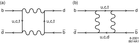
Figure 1: Leading Diagrams for $B\overline{B}$ Mixing in the Standard Model

1.3 The Three Types of $CP$ Violation

In the above discussion we have already mentioned two possible ways that $CP$ violation can occur. The first was $CP$ violation in the decay, or direct $CP$ violation, which requires that two $CP$-conjugate processes to have differing absolute values for their amplitudes. A second possibility, seen for example in $K$ decays, occurs if $|q/p|\neq 1$. It is very clear in this case that no choice of phase conventions can make the two mass eigenstates be $CP$ eigenstates. This is generally called $CP$-violation in the mixing. As we will see later, in decays of the neutral mesons to a $CP$-eigenstate $f$, there is a third possibility. This can occur even when both the ratio of amplitudes and the quantity $q/p$ have absolute value 1. The $CP$ violation effects in such decays will be shown to depend only on the deviations from unity of the parameter $\lambda_{f}=(q/p)A(\overline{B}^{0}\rightarrow f)/A(B^{0}\rightarrow f)$ . The third option is $CP$ violation in the interference between decays to $f$ with and without mixing. This effect is proportional to the imaginary part of $\lambda_{f}$ and thus can be non-zero even when the absolute value satisfies $|\lambda_{f}|=1$. Decays where this latter condition is true are particularly interesting. In such cases one can interpret any observed asymmetry as a direct measurement of some difference of phases of CKM matrix elements, with no theoretical uncertainties. We will see this in more detail in the next lecture.

2 Lecture 2: Standard Model Predictions for $CP$ Violations in $B$ Decays

2.1 CKM Unitarity

The CKM matrix of quark weak couplings has been discussed in some detail in previous lecture series in this school. It can be written, in the Wolfenstein parameterization [9], as

$$V = \pmatrix{V_{ud}&V_{us}&V_{ub}\cr V_{cd}&V_{cs}&V_{cb}\cr V_{td}&V_{ts}&V_{tb}}$$ (8)

$$\simeq \pmatrix{1-\lambda^{2}/2&\lambda&A\lambda^{3}(\rho-i\eta)\cr-\lambda&1-\lambda^{2}/2&A\lambda^{2}\cr A\lambda^{3}(1-\rho-i\eta)&-A\lambda^{2}&1}+O(\lambda^{4})~{}.$$

In the previous lecture I talked about the ability to remove, or move, a complex phase of a coupling by redefining the phase of any field involved. This parameterization corresponds to a particular choice of phase convention which eliminates as many phases as possible and puts the one remaining, possibly large, complex phase in the matrix elements $V_{ub}$ and $V_{td}$.

In this convention the upper right off-diagonal elements define the parameters. The parameterization is a convenient way to make the unitarity of the matrix explicit, up to higher order corrections in powers of $\lambda\equiv V_{us}$. (The higher order terms may also have phases, as required by the unitarity relationships, but bring in no new independent phase parameters.) The quantity $\lambda$ is essentially the sine of the Cabibbo angle. It is a small number, of order 0.2. Wolfenstein’s parameterization uses powers of $\lambda$ is a convenient way to keep track of the relative sizes of the terms in the matrix. The other independent magnitude parameters $A$ and $\rho^{2}+\eta^{2}$ are known to be roughly of order unity. There is no theory behind which powers of $\lambda$ enter each term. The Wolfenstein parameterization simply summarizes the observations in a neat way. The fact that $V_{cb}$ and $V_{ub}$ are both small (of order $\lambda^{2}$ and $\lambda^{3}$ respectively in Wolfenstein’s parameterization) is responsible for the relatively long lifetimes of $B$-mesons (and $b$-containing baryons too). This is a fortunate property; it is essential to the feasibility of most $B$-physics experiments because it allows us to identify $B$ decays by the spatial separation of the decay vertex from the production point. It is an observational fact, not a theoretical prediction.

Independent of the parameterization used, in the three generation Standard Model the CKM matrix must be unitary. This leads to a number of relationships among its elements of the form [(row)*x(column)]=0. Examples are

$$V_{ud}V^{*}_{us}+V_{cd}V^{*}_{cs}+V_{td}V^{*}_{ts} = 0\hskip 36.135pt{a}$$

$$V_{us}V^{*}_{ub}+V_{cs}V^{*}_{cb}+V_{ts}V^{*}_{tb} = 0\hskip 36.135pt{b}$$ (9)

$$V_{ub}V^{*}_{ud}+V_{cb}V^{*}_{cd}+V_{tb}V^{*}_{td} = 0\hskip 36.135pt{c}\ .$$

In the Wolfenstein parameterization the relationship that arises from unitarity can be used to express the diagonal and lower left hand elements of the matrix in terms of the upper right elements, to any desired order in $\lambda$. The form given above drops terms of order $\lambda^{4}$ and above.

It is a trivial fact that any relationship of the form of a sum of three complex numbers equal to zero can be drawn as a closed triangle in the complex plane. Hence these, and the other similar relationships, are referred to as the Unitarity Triangle relationships. The fact that there is only one independent $CP$-violating quantity in the CKM matrix can be expressed in phase-convention-invariant form by defining the quantity $J$, called the Jarlskog invariant for Cecilia Jarlskog who first pointed out this form [10],

$${\rm Im}V_{ij}V_{kl}V_{il}^{*}V_{kj}^{*}=J\Sigma_{m,n=1}^{3}\epsilon_{ikm}\epsilon_{jln}$$ (10)

where $i,j,k,l$ run over the values $1,2,3$ and $\epsilon_{ijk}$ takes the value +1 if the three indices are all different and in cyclic order, and -1 if they are all different and in anti-cyclic order, but is zero if any two are the same. All the unitarity triangles have the same area, $J/2$. This area shrinks to zero if the $CP$-violating phase differences in the matrix vanish.

Notice however that, while the triangles have the same area, the three examples given above are triangles of very different shapes. Triangle ${a}$ has two sides of order $\lambda$ and one of order $\lambda^{5}$. It would be very difficult to measure the area using such a triangle. Triangle ${b}$ is a little better, but still a has one small angle, its larger sides are of order $\lambda^{2}$ while its small side is of order $\lambda^{4}$ giving an angle of order $\lambda^{2}$. Finally triangle ${c}$ is the most interesting, because it has all three sides of order $\lambda^{3}$ so all three angles are a priori of comparable and large magnitude. The price one pays is that all the sides are small, but this is not as serious as the problem of measuring an asymmetry proportional to a very small angle. This triangle is the one most often discussed in relation to $B$-meson decays. Since these angles are large one expects some channels in both $B_{d}$ and $B_{s}$ decays with order 1 $CP$-violating asymmetries .

2.2 Fixing the Parameters

The triangle is conventionally drawn by dividing all sides by $V_{cb}V_{cd}^{*}$, which gives a triangle with base of unit length whose apex is the point ($\rho,\eta$) in the complex plane. Prior to considering the asymmetry measurements we can try to determine the shape of this triangle from measurements of $CP$-conserving quantities which fix the sides, plus the measured $CP$ violation in $K$-decays. Notice that this information is already sufficient (in principle) to over constrain the set of parameters.

The quantity $V_{cb}$ is determined from $B$ decays to charmed final states, $V_{ub}$ from final states with no charm, while measurements of the $B_{d}$ and $B_{s}$ mass differences constrain $V_{td}$. The $CP$ violation in $K\rightarrow\pi\pi$ gives an allowed band for the apex of the triangle. In each case there is both an experimental uncertainty in the measurement and a theoretical uncertainty in the relationship between the measured quantity and the theoretical parameter(s). The theoretical uncertainties dominate. They are typically not statistical in nature, but rather have to do with the part of the calculation which involves models or approximations needed to allow for strong interaction physics effects. There is a large literature by now on the topic of how best to combine the various measurement and deal with both statistical and theoretical uncertainties [11].

New measurements from Belle and BaBar on a $CP$ asymmetry in $B$-decays constraining the angle at the lower left of the triangle have recently been announced [12]. This is one measurement where the theoretical uncertainties are very small, so the constraint will improve as the statistics of the measurement improve for some time to come. So far all the various results give a consistent picture; the Standard Model fits the data. This means that, within the ranges of the various theoretical uncertainties, there is a region of possible choices for the Lagrangian parameters that are consistent with all data.

One hope of many physicists involved in the large effort in $B$ physics is that at some point some measurements will give discrepant answers for some Standard Model parameters or predictions. This would be evidence for physics beyond the Standard Model, and cause for much excitement in the physics community. If results for some set of measurements should begin to look discrepant, then the question of the statistical significance of the discrepancy will be much debated, as different treatments of theoretical uncertainties will give different conclusions on this point.

Let us examine one of these quantities in a little more detail to see how the theoretical uncertainties arise. In each case there is a mix of weak interaction and short-distance strong-interaction physics, which both are perturbatively calculable and long range strong-interaction physics which is not perturbatively calculable. Tomorrow’s lecture will introduce some of the methods that are used to deal with (or avoid) possible long-range strong interaction effects. Here I simply want to show how such effects can enter. Consider the question of the mass difference between the two mass eigenstates for $B_{d}$. The two one-loop diagrams given in Fig. 1 are the dominant contribution to this effect. Each loop-diagram can have either a $t$-, $c$-, or $u$-quark for each of the two internal quark lines. Calculation of the matrix element of these diagrams between a $B^{0}$ and a $\overline{B}^{0}$ meson would give $M_{12}+i\Gamma_{12}/2$.

The diagrams can be written as a local four-quark operator multiplied by a calculable coefficient which includes CKM factors. I will write the quark-propagator and coupling dependent part of this coefficient schematically as

$$Q=|V_{td}V_{tb}^{*}D_{t}+V_{tcd}V_{cb}^{*}D_{c}+V_{ud}V_{ub}^{*}D_{u}|^{2}$$ (11)

where the $D_{q}$ factors are the quark propagators. This expression is schematic because in writing it as a perfect square I ignored the differences in the momenta of the two quark lines in the diagram (which are typically small, ${\cal{O}}(m_{b}/m_{W})$, compared to the loop momentum itself).

Notice that if all the quarks had equal mass then $D_{t}=D_{c}=D_{u}$ and the unitarity condition Eq. (2.1c) would say that this factor $Q$ vanishes. Indeed we can use this condition to rewrite the expression as

$$Q=|V_{td}V_{tb}^{*}(D_{t}-D_{u})+V_{cd}V_{cb}^{*}(D_{c}-D_{u})|^{2}.$$ (12)

Because of the two $W$-propagators the loop integral is dominated by momenta of order $M_{W}$, which is large compared to either the $c$ or $u$ quark masses. Thus the two quark propagators in the second term of Eq. (12) above essentially cancel one-another, so the term is suppressed by a factor of order ${(M_{c}^{2}-M-u^{2})}/{m_{W}^{2}}$. Thus the mass difference is effectively proportional to the square of the coefficient of the remaining term, which $|V_{td}|^{2}$ (since $V_{tb}$ is 1 up to order $|\lambda|^{4}$). (Note that this argument also shows why the mixing matrix is small in the $D$-meson case. There the three propagators are the down-type quarks, all three of which have masses that are small compared to $M_{W}$, so the Unitarity cancellations suppress the entire effect. Furthermore the contribution of the most-massive quark in this case, the $b$-quark, is Cabibbo-suppressed, further reducing the effect. )

To find the value of this $V_{td}$ by measuring the $B$ meson mass differences we need to know the matrix element of the four quark operator between the $B^{0}$ and $\overline{B}^{0}$ meson states. This is where the long-distance hadronic physics sneaks into the problem, this matrix element depends on the form of the $B$ wavefunction, including all effects of soft gluons. The best available method to determine it is to use lattice QCD calculation [13].

A measurement of the mass difference of the two $B_{d}$ mass eigenstates thus gives a measurement of $V_{td}$ with a theoretical uncertainty that is dominated by the theoretical uncertainty in the lattice determination of the relevant four-quark matrix element. The result is usually written as some “known” factors times $B_{B}f_{B}^{2}$. (The “known” factors include quark masses, which are actually not so well-known and must be carefully defined.) Here the factor $f_{b}^{2}$ is the vacuum to one meson matrix element of the axial current which arises in the naive approximation to the matrix element obtained by splitting the four-quark operator into two-quark terms and inserting the vacuum state between them. This is known as the vacuum-insertion approximation. The quantity $B_{B}$ is simply the correction factor between that approximate answer and the true answer. It can be estimated in various model calculations. The lattice calculation does not need to make this subdivision, it directly calculates the full matrix element. However the result is often quoted in terms of the $B_{B}$ and $f_{B}$ parameters. Lattice methods can also directly calculate the latter. Eventually $f_{b}$ will be measured and that will provide a separate test of the lattice calculation.

Once there is a good measurement of the $B_{s}$ mass difference the ratio $\Delta m_{b}/\Delta m_{s}$ will provide a better determination of $V_{td}$ via the ratio $V_{td}/V_{ts}$. This mass ratio is relatively free of theoretical uncertainties, as most of these cancel in the ratio of matrix elements. The matrix elements for the $B_{d}$ and the $B_{s}$ mesons are similar. Only a small correction due to the difference of the $s$ and $d$ quark masses remains. The uncertainty in this correction gives a relatively small theoretical uncertainty in $V_{td}$. At present only a lower limit for the $B_{s}$ mass difference is known; even this gives an important constraint (upper limit) on the range of $V_{td}$.

2.3 Time Evolution of the $B$ States and Time-Dependent Measurements

Now I turn to the topic of decays of neutral $B$ mesons. What can we measure and what does it tell us? To discuss this we need to understand the time evolution of state which at time $t=0$ is known to be a pure $B^{0}$ meson. This means that at t=0 we have

$$B(t=0)=(B_{H}+B_{L})/2p\ .$$ (13)

Since the two mass states evolve with different time-dependent exponential prefactors we find

$$B(t)=g_{+}(t)B^{0}+(q/p)g_{-}(t)\overline{B}^{0}$$ (14)

where the functions $g_{\pm}$ are just the sums and differences of the exponential mass and lifetime factors

$$g_{\pm} = [e^{(-iM_{H}t-\Gamma_{H}t/2)}\pm e^{(-im_{L}t-\Gamma_{L}t/2)}]/2$$ (15)

$$= e^{-iMt-\Gamma t/2}[e^{(-i\Delta M-\Delta\Gamma/2)/2}\pm e^{(i\Delta M+\Delta\Gamma/2)/2}]/2\ .$$

Here we introduce the notation $M$ and $\Gamma$ for the average mass and width and $\Delta M$ and $\Delta\Gamma$ for the differences between the two sets of eigenvalues. In the case of $B_{d}$ the width difference is small compared to the mass difference (and to the width itself) so to a good approximation we can neglect $\Delta\Gamma$. Then the expressions for the $g_{\pm}$ simplify in an obvious way. For $B_{s}$ it is likely that the width difference is comparable to the mass difference and the full expressions must be used.

The time-dependent state that is a pure $\overline{B}^{0}$ at $t=0$ can likewise be written in terms of these same functions

$$\overline{B}(t)=(p/q)g_{-}(t)B^{0}+g_{+}(t)\overline{B}^{0}.$$ (16)

It is now straightforward to derive the time-dependent rate to reach a particular $CP$ eigenstate final state $f$ with $CP$ quantum number $\eta_{f}$. It is given by

$$|A(B(t)\rightarrow f|^{2}=|A(B^{0}\rightarrow f)|^{2}[|g_{+}(t)|^{2}+|\lambda_{f}g_{-}(t)|^{2}+2Re[g^{*}_{+}(t)g_{-}(t)\lambda_{f}]]$$ (17)

where the quantity

$$\lambda_{f}=(q/p){A(\overline{B}\rightarrow f)\over A(B\rightarrow f)}=\eta_{f}(q/p){A(\overline{B}\rightarrow\overline{f})\over A(B\rightarrow f)}.$$ (18)

In the second equality here we have used the fact that f is a $CP$ eigenstate, $CPf=\overline{f}=\eta_{f}f$ where $\eta_{f}=\pm 1$, to write the ratio of amplitudes in a form that shows explicitly that one amplitude is simply the $CP$ conjugate of the other.

The $CP$-violating asymmetry between the rates is defined to be

$$a(t)={|A(\overline{B}(t)\rightarrow\overline{f})|^{2}-|A(B(t)\rightarrow f)|^{2}\over|A(\overline{B}(t)\rightarrow\overline{f})|^{2}+|A(B(t)\rightarrow f)|^{2}}\ .$$ (19)

(Note once again you must beware of conventions, some of the literature defines the asymmetry with the opposite sign.)

If $\Delta\Gamma/\Gamma$ can be neglected, which is a very good approximation for $B_{d}$ decays, then $|q/p|=1$ and the asymmetry takes the form

$$a(t)=-[(1-|\lambda_{f}|^{2})\cos(\Delta Mt)+2Im\lambda_{f}\sin(\Delta Mt)]/(1+|\Lambda_{f}|^{2})\ .$$ (20)

As promised previously, this relationship shows that the $CP$-violating effects measure properties of $\lambda_{f}$, in particular its magnitude and imaginary part. (In the more general case the expressions are somewhat more complicated and depend also on the width difference.) In particular, if only the third type of $CP$ violation is present, namely if in addition to $|q/p|=1$ we have $|\overline{A}/A|=1$ so that $|\lambda_{f}|=1$, then this expression simplifies to

$$a(t)=-Im\lambda_{f}\sin(\Delta Mt)]\ .$$ (21)

The argument of $\lambda$ depends simply on weak phases, so that

$$Im\lambda_{f}=\eta_{f}\sin(2\phi_{\rm mixing}-2\phi_{\rm decay})\ .$$ (22)

Here $2\phi_{\rm mixing}$ is the phase of $q/p$ and $2\phi_{\rm decay}$ is the phase of $A(\overline{B}\rightarrow\overline{f})/A(B\rightarrow f)$ while $\eta_{f}$ is the $CP$ quantum number of the state $f$. These phases are each given by some combination of $CKM$ matrix-element phases. While each of them separately can be changed by changes in phase convention (rephasing of quark fields) the difference is convention independent, as must be so for any physically measurable quantity. Thus the asymmetry directly measures the phase differences between particular CKM matrix elements with no uncertainties introduced by our inability to calculate strong interaction physics effects such as the magnitude or strong phase of an amplitude. These strong interaction effects all cancel exactly when $|\lambda_{f}|$ is 1.

2.4 CP Eigenstate Channels for $b\rightarrow c\overline{c}s$

There are many possible channels to investigate. The interest lies not just in one measurement but in whether the pattern of $CP$-violating asymmetries fits the predictions of the Standard Model. What channels should we study? We need a final state of definite $CP$. In general for a multibody final state even when the particle content is $CP$-self conjugate there will be an admixture of $CP$-even and $CP$-odd contributions because of different possible orbital angular momenta among the particles. The simplest way to get a definite $CP$ final state is to require that the $B$ decay to a two-body or quasi-two body final state with only one allowed orbital angular momentum. (Quasi-two-body here simply means a two-body state with one or two unstable particles, such as a $\rho\pi$ or $\rho\rho$. The actual observed final state is then three or four pions.) Given that the $B$ has spin zero, the final state has a unique orbital angular momentum between the pair of particles if (and only if) at least one of the two particles has spin zero. For quasi-two body states where both particles have non-zero spin but at least one of them is unstable one can possibly separate out the $CP$-even and $CP$-odd final state contributions using an angular analysis of the distribution of secondary decay products [14]. The price is that, in general, a larger data sample is needed to achieve the same accuracy on the $CP$ asymmetry measurement.

Note that the Feynman diagram structure is the same for all channels with the same quark content. Results from multiple channels can sometimes be combined to improve statistical accuracy. For example for the quark decay $b\rightarrow c\overline{c}s$ the $B^{0}$ decay channels $J/\psi K_{S},\psi^{\prime}K_{S},\eta_{c}K_{S}$ $J/\psi K_{L},\psi^{\prime}K_{L},\xi_{c}K_{L}$ (etc.) all depend on the same set of quark diagrams. For the $b\rightarrow u\overline{u}d$ (and $d\overline{d}d$)quark content there are likewise many channels: $\pi\pi,\rho\pi,\rho\rho$, etc. (The last of these needs angular analysis.)

Let us then examine what the predicted $CP$ asymmetry is in each of these two cases. We begin with the modes such as $B\rightarrow J/\psi K_{s}$. These have been called the golden modes for analyzing $CP$ violation in $B$ decay. For once we have a situation where the mode for which the theoretical analysis is straightforward is also one with good experimental accessibility. One still needs a large sample of $B$ decays because the branching fraction to these channels is not large. (In $B$ decays there are so many open channels that branching fractions are small and smaller: the “large” modes occur at the few percent level; $J/\psi K_{S}$ and similar modes are about a tenth of a percent; a “rare” mode in this game has a branching fraction a few times $10^{-5}$.)

First we need a little terminology. We use the term spectator quark for the quark other than the $b$-type quark (or antiquark) that is present in the initial $B$ meson, since it is generally not involved in the $b$-decay diagram. There are two topologies of weak decay Feynman diagram that can contribute to $B$ decays to leading order in the weak interactions. These are called “tree” and “penguin” diagrams and are shown in Fig. 2. A tree diagram is one where the $W$-boson creates or connects to a different quark line from the line that starts out as the $b$-quark. I thus also include any annihilation diagram or any diagram where the $W$-boson connects to the spectator quark as part of what I call the tree amplitude. Whenever such a diagram is allowed it will enter with the same CKM factors as the other tree diagram processes. A penguin diagram is a loop-diagram where the $W$ reconnects to the quark line from which it was emitted. Then a hard gluon is emitted from the quark line in the loop, and either makes a pair or is absorbed by the spectator quark.

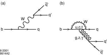
Figure 2: The (a) tree and (b) penguin weak decay processes at the quark level.

When higher order strong interaction rescattering effects are included the distinction between tree and penguin diagrams becomes blurred. However, it is useful (and standard) to start out by describing processes in this language as it allows us to identify all the relevant CKM factors, and the operators which they multiply. As we will shortly see, that is the essence of the story. Eventually we will group terms not by the diagrams, but by the CKM factors. That grouping is not blurred by any subsequent strong interactions. The language tree and penguin persists, but the “tree contribution”, in my terminology will be taken to include not only the tree diagrams (including those that involve the spectator in the weak vertex), but also that part of the contribution from the penguin diagrams that has the same CKM factor as the tree diagrams. Obviously, if one wants to try to calculate the size of the contribution to the amplitude one must keep track of each diagram separately, but if we are only concerned with whether there is more than one CKM structure in the significant contributions we can lump together all the terms with a given CKM factor.

The cleanest cases theoretically are those where we can make a prediction without knowing anything about the sizes of the amplitudes because we are looking at a ratio of rates where these cancel to a good approximation. The $CP$-violating asymmetry in channels arising from quark transition $b\rightarrow c\overline{c}s$ in a $B_{d}$ meson is just this type. The tree diagram has a CKM factor $V_{cb}^{*}V_{cs}$. Any time that penguin diagrams contribute to an amplitude there are three terms, corresponding to the three different up-type quarks that inside the loop. Thus we can write the $b$ to $s$ penguin amplitude $P$ in the form

$$P = V_{tb}^{*}V_{ts}f(m_{t})+V_{cb}^{*}V_{cs}f(m_{c})+V_{ub}^{*}V_{us}f(m_{u})$$ (23)

$$= V_{cb}^{*}V_{cs}[f(m_{c})-f(m_{t})]+V_{ub}^{*}V_{us}[f(m_{u})-f(m_{t})]$$

where the $f(m_{q})$ is some function of the quark mass. In the second expression I have once again used the Unitarity relationship Eq. (2.1c) to rewrite the three terms in $P$ in terms of two independent CKM factors. Notice that the first of these is the same as that for the tree term, so for this discussion we call that contribution part of the “tree amplitude”. The remaining term is CKM suppressed by an additional factor of $\lambda^{2}$. The two differences of quark-mass-dependent factors are expected to be comparable in magnitude. Furthermore, ignoring CKM factors, the penguin graph contribution is expected to be suppressed by about 0.3 compared to the tree graph, because it is a loop graph and has an additional hard gluon. This means the suppressed second term in Eq. (23) is negligible (a few percent) compared to the “tree amplitude” which here is the sum of the tree term and the dominant penguin term.

Thus we have an amplitude that effectively has only a single CKM coefficient and hence one overall weak phase. This then ensures $|\overline{A}/A|=1$, which means there is no decay-type (direct) $CP$ violation. (You will recall we needed two terms with different weak phases to get such an effect. ) Remember too that for $B_{d}$ we expect $|q/p|=1$ to a good approximation. Thus we have a case where $|\lambda_{f}|=1$ and the measured asymmetry arises purely from the interference of decay before and after mixing. We find

$$a_{J/\psi K_{S}}=-Im(\lambda_{J/\psi K_{S}})\sin(\Delta Mt)=\sin(2\beta)\sin(\Delta Mt)\ .$$ (24)

Here the quantity $\beta$ is the lower left-hand angle in the standard $B$ physics Unitarity triangle (also sometimes called $\phi_{1}$). (The minus sign disappears because $\eta_{f}=-1$ for $f=J/\psi K_{S}$.) Thus this asymmetry directly measure the phase of a rephasing-invariant combination of CKM elements.

Furthermore all the channels in the $c\overline{c}s$ list above measure the same asymmetry, up to an overall sign, the $\eta_{f}$ factor of the channel in question. For example $K_{S}$ and $K_{L}$ are states of opposite $CP$, as are the $\psi$ and $\eta_{c}$. Care must be taken to include the correct $\eta_{f}$ factor for each state in combining the results. One can also include a state such as $J/\psi K^{*}$ provided the $K^{*}$ decays to a flavor-blind combination such as $K_{S}\pi^{0}$, and angular analysis is used to separate $CP$-even and $CP$-odd contributions.

One can apply this same diagrammatic analysis to the decays $b\rightarrow c\overline{c}s$ in a $B_{s}$ meson. This gives a prediction for channels such as $J/\psi\phi$ that the $CP$ asymmetry is zero in the Standard Model, as the $B_{s}$ mixing term is dominated by CKM factors with the same weak phase as this decay. Thus, in the Standard Model, only the CKM suppressed penguin terms which we neglected above can give $CP$ violating asymmetries here, so at most a few percent asymmetry is expected. Such predictions of small or vanishing asymmetries give another way to examine the patterns of the Standard Model. Any theory of new physics effects which give additional mixing contributions could destroy the cancellation of mixing phase and decay phase which makes this asymmetry small in the Standard Model. However to interpret such a result one indeed needs some calculation of decay amplitudes, in order to quantify more precisely how big the “few percent” Standard Model asymmetry could be.

The trick of rewriting the sum of three penguin terms as two terms using the Unitarity relationships is a generally useful tool. In any channel one then has at most two CKM factors to consider. The next step is to get a rough estimate of the relative size of the two terms. This becomes important when $|\overline{A}/A|\neq 1$.

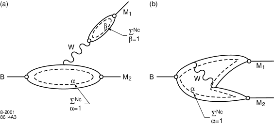
Figure 3: Possible two-meson tree-diagram decay processes showing color-flow loops as dotted lines. These are called (a) color-allowed tree contribution, and (b) color suppressed tree contribution.

2.5 Some further $B$ Physics Jargon

The $B$ physics jargon distinguishes contributions by three attributes, because these three things give a first estimate of how big the contribution is. The first size factor is whether the diagram is tree or penguin. The penguin is suppressed relative to the tree because it is a loop diagram and because it involves a factor of $\alpha_{\rm strong}$ at a scale of order $m_{b}$ due to the hard gluon, together this makes for a suppression factor of order about 0.3, all else being equal. The next size factor is the powers of the Wolfenstein parameter $\lambda$ in the associated CKM factors. All $B$-decay amplitudes have at least two powers of $\lambda$. Amplitudes with higher powers are called CKM-suppressed. The third size factor is the color flow pattern that forms the particular final state of interest. Diagrams where a quark-antiquark pair produced by a W finish up in the same meson are called color-allowed, because this pair is produced in the requisite color-singlet combination. In terms of color-flow diagrams there are two independent color-flow loops as shown in Fig. 3(a). When the quark and antiquark produced by the $W$ end up in different final mesons the diagram is called color-suppressed (Fig. 3(b)). There is then only a single color-flow loop so that diagram is expected to be of the order of $1/N_{c}$ smaller than the corresponding color-allowed diagram.

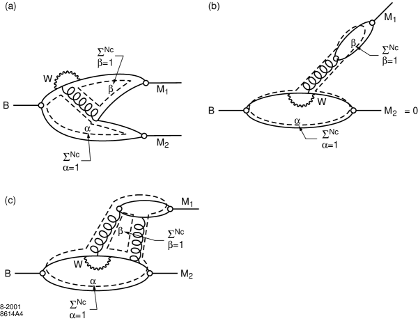
Figure 4: Possible penguin-type two-meson decay processes showing color-flow loops as dotted lines. These are called (a) color allowed penguin, (b) naive color suppressed penguin process, vanishes exactly, and (c) allowed diagram with additional gluon for so-called color-suppressed penguin process. (It has two color flow loops as does the “color-allowed”, but an additional $\alpha_{qcd}$ factor.)

For penguin diagrams color suppression, if it works at all, works the other way around. Diagrams where the quark and antiquark from the gluon end up in two different mesons, Fig. 4(a), are color allowed, and indeed can be seen to have two-color-flow loops just as do the tree color-allowed contributions. Diagrams where the flavor-structure says the quark and antiquark produced by the hard gluon must be in the same meson are called color suppressed. In Fig. 4(b) there is only one color loop. However in this diagram the gluon makes a color singlet object. But a gluon is a color-octet state. Taken literally, the diagram vanishes. A second gluon must be exchanged here. If we were to count the extra gluon as a hard gluon, there would be an additional suppression factor of $\alpha_{\rm strong}$, but no $1/N_{C}$, because we would again see two color loops, Fig. 4(c). However the second gluon is not necessarily hard, so the relevant scale for the $\alpha_{\rm strong}$ is not large. In some estimates these contributions are treated as $1/N_{C}$ suppressed terms, but there is no good argument that justifies this counting. As you can see from these arguments, the naive color-counting is not a very reliable measure of the relative strengths of the two types of penguin contributions. QCD-improved operator-product expansion calculations at leading order in $\Lambda/m_{b}$ [15, 16, 17] can be made. These treat the color factors correctly. We will return to this approach at later, in Lecture 3. However there is a large literature of estimates that use the language of color-allowed and color-suppressed contributions, so it is important to know how these terms arose and how they are used.

All these size-counting factors are generally used to give first estimates of the order of magnitude of the various contributions. Clearly a more serious calculation can significantly change the relative sizes. The kinematics of the different diagrams are different. The matrix elements of the various operators are different. Indeed there is an interplay between the wave function of the mesons and the counting factors discussed above which in the end determines the size of an amplitude. Powers of $\Lambda_{QCD}/m_{b}$ can arise from the wavefunction for particular kinematic configurations relative to others. Higher-order hard QCD effects can be systematically included, but the soft hadronization part of the calculation needs some additional input, either from a model or from some other measurement.

2.6 Another Sample Channel

Now let us look at one more set of channels to see what happens when this size counting says two CKM factors can occur with comparable coefficients. The case I choose to examine is the decay $B_{d}\rightarrow\pi^{+}\pi^{-}$. At the quark level this process is governed by decays $b\rightarrow u\overline{u}d$. You can readily find from the diagrams of Fig. 2 that there are both tree and penguin contributions for this quark content. The tree diagrams have a CKM factor $V_{ub}^{*}V_{ud}$. For the penguin contributions we can again use unitarity to rewrite the three different intermediate quark contributions as a sum of two terms. In this case all three CKM coefficients are of the same magnitude. I choose to eliminate $V_{cb}^{*}V_{cd}$ because then the second penguin term (the one that does not have the same weak phase as the tree term) has the same weak phase as the mixing term in the Standard Model. Then only one difference of CKM phases will enter my eventual formulae for the asymmetry. However we cannot ignore the second penguin term. The only thing that makes it small compared to the “tree amplitude” (which includes the first penguin term as well as the contribution from the tree diagram) is the fact it is a penguin loop. That is not sufficient to completely discard it.

So here we have a situation where there can be $|\overline{A}/A|\neq 1$ effects. We must use Eq. (20) to interpret the the measured asymmetry. One would like to extract from the measurement the CKM phase difference between mixing and tree decay contribution (which in this case is $\alpha\equiv\pi-\beta-\gamma$). One can measure two quantities, $|\lambda_{f}|$ from the coefficient of cos($\Delta Mt$), and Im$\lambda_{f}$ from the coefficient of sin($\Delta Mt$).

However three unknown quantities enter in the expressions for $\lambda_{f}$ in such a case. These are the relative weak phase of mixing and the tree decay amplitude $\alpha$, and both the absolute value ratio, r, and the relative strong phase, $\delta$ of the penguin and tree terms. We can write

$$\lambda_{f}=e^{-2i\alpha}{1+re^{i(\delta+\alpha)}\over 1+r^{i(\delta-\alpha)}}\ .$$ (25)

Here the phase $\alpha=\pi-\gamma-\beta$ is the angle at the top vertex of the standard $B$-physics unitarity triangle; it is the difference between the weak phases of the mixing and that of the tree contribution to the decay. Obviously, knowledge of both the real and imaginary parts of $\lambda_{f}$ is not enough to fix all three quantities. So we cannot extract a value of $\alpha$ from this asymmetry measurement alone. (Note, however that for very small r the expression simplifies so that the measurement of Im$\lambda$ determines sin$2\alpha$.) We must use further theory or measurement inputs (or both) to determine $\alpha$ if r is not small. (A note of warning here, one often sees the statement that one tests the Standard Model by testing the relationship $\alpha=\pi-\beta-\gamma$ between the angles in the triangle. The relationship is a definition. The tests of the Standard Model are tests of whether one finds the same result for the two independent angles, usually chosen to be $\beta$ and $\gamma$, using a variety of independent ways to measure them.)

Note also that the ratio, $re^{i\delta}$, of the tree to the penguin amplitudes will be different for the different channels with the same quark content. The kinematics of the tree and penguin diagrams are different, and so are the wave functions for forming a $\pi$ or a $\rho$, for example. Thus, unlike the $c\overline{c}s$ decays, we cannot simply combine channels to improve statistical accuracy. Instead we must devise methods to remove the dependence on the additional parameters; these methods are different for each set of final state particles.

For the $\pi\pi$ case there are two ways to proceed. One is to rely on isospin symmetry and isospin-related channels to give the needed additional information. The second is to develop methods to calculate these various amplitudes more reliably. This may also involve using relationships to other channels where the tree and penguin amplitudes enter with different relative strengths because of different CKM structure. For example by using measurements on $K\pi$ channels as well with those from $\pi\pi$ channels one can gain some information on the size of the penguin amplitude which dominates the decay in the former case. One can then use SU(3) symmetry to relate that to the size of the penguin in the $\pi\pi$ case. Eventually such methods can much reduce the theoretical uncertainty in the extraction of the CKM parameter $\gamma$, or equivalently $\alpha=\pi-\beta-\gamma$. Tomorrow I will discuss both of these approaches in a little more detail.

The set of all possible $B$ decays can be summarized by reviewing all possible $b$-quark decays and the channels to which they can contribute. A little care must be applied to this logic, as strong rescattering can turn one quark-antiquark combination into another, one must include this possibility in a full treatment. For example in any channel involving a $\pi^{0}$ or $\rho^{0}$ meson the penguin diagrams for $b\rightarrow d\overline{d}d$ must be added to the diagrams for $b\rightarrow u\overline{u}d$. I refer you to the table in the Particle Data Book review on this topic [18] that summarizes the quark decays and gives the CKM factors that enter for each (after using the Unitarity trick to get two terms only.) Any time you start thinking about a specific process you will find you want this information. You can rederive it readily by drawing the allowed quark diagrams and investigating their CKM factors.

3 Lecture 3. Theorist’s Tools for $B$-physics

Today’s lecture will briefly introduce a number of theoretical tools for calculating $B$ decay processes. There are only a few examples of measurements for which we do not need to know the relative magnitude of various contributions to the decay amplitudes in order to relate the measurement to some parameters in the theory. We would like to go further and interpret the multitude of other measurements that are possible because of the many different $B$-decay channels. To do this we must devise methods to calculate or relate amplitudes. The available calculational methods all involve some mix of systematic expansion in powers of one or more small parameters, lattice calculation of matrix elements of operators, relationships based on symmetries of the strong interactions such as isospin and SU(3) flavor symmetry, and some input for transition matrix elements and or quark distribution functions. These last can be calculated reliably only in certain limits and in general require models and approximations. Alternately one can measure some of these quantities in one set of processes and use the measured values as input in the interpretation of other measurements.

This lecture will give a general picture of the toolkit of approaches, what each tool is, and how it can be used. There will not be time here to teach the details of any of the methods. This lecture summarizes a large body of theoretical work. I will not attempt to reference all the relevant papers, but will include references to some current papers as examples of the type of work now underway. I apologize in advance to the many whose papers I do not mention.

There are two small parameters in this game, namely $\Lambda_{QCD}/m_{b}$ and $\alpha_{\rm strong}(m_{b})$. Here $m_{b}$ is the mass of the $b$-quark and $\Lambda_{QCD}$ is the scale that defines the running of the strong interaction coupling. The detailed definition of each of these quantities is fraught with technical problems, but there is a clear physical meaning for the rough size of these parameters. $\Lambda_{QCD}$ is related to the inverse size of a typical hadron while the $b$-quark mass can be characterized as roughly the same scale as the mass of a $B$ meson (up to corrections of order $\Lambda_{QCD}/m_{b}$). The strong coupling $\alpha_{s}(m_{b})$ scales as a logarithm of $\Lambda_{QCD}/m_{b}$; we treat it as a separate small parameter because we can count powers of this parameter separately from the powers of $\Lambda_{QCD}/m_{b}$; they arise in different ways.

The fact that $\Lambda_{QCD}/m_{b}$ is indeed quite small leads to a simple intuitive picture of a $B$ meson at rest. It is an essentially static $b$ quark with the light quark forming a cloud around it. The light-quark distribution is sometimes called the brown muck, because we cannot reliably calculate the details of it. However we do know that certain properties are rigorously true in the limit $m_{b}\rightarrow\infty$. For example in that limit the wavefunction does not depend on the spin orientation of the $b$-quark and hence is the same for a spin 0 $B$ meson and a spin 1 $B^{*}$. A second way in which the large mass of the $b$-quark simplifies the problem is that any gluon that carries off a significant fraction of the $b$-quark mass is a hard gluon that can be treated perturbatively; it introduces the small parameter $\alpha_{\rm strong}(m_{b})$.

In addition to these expansions there is another part of the picture that is true because $m_{b}/M_{W}$ is small. This means that weak decays of the $b$-quark are essentially local four-quark effects. Thus the $B$ meson decay can, to a reasonable approximation, be thought of as proceeding in two stages: a $b$-quark decays and then the remnants hadronize to give the final state under study. It is this second stage, the hadronization, that introduces all the uncertainties into the calculations. We have good methods for applying QCD to things like jet-formation for well-separated high momentum quarks, but a $B$ decay does not give us large enough quark momenta to use this formalism reliably. Further, we want to know amplitudes for specific few-body (quasi-two-body) final states (states of definite $CP$). Most likely these arise when the four quarks that are present after the $b$ decay are not well-separated (so even if the $B$ mass were much larger a jet calculation would not provide the answer). We cannot calculate these amplitudes completely from first principles. So my purpose in this lecture is to review the tools that we do have and how they can be used to minimize the theoretical uncertainty on the extraction of the desired quantities, such as CKM parameters, from experiment.

3.1 Operator Product Expansion

The operator product expansion is a way to formalize the separation of hard or short-distance physics from soft or long-distance physics. It begins by rewriting the Feynman diagrams into the form of local operators, defined at a given scale, with calculable, scale-dependent coefficients.

First we look at all the tree and penguin Feynman diagrams for the weak decay of the $b$-quark. Each can be written as a sum of four quark operators with definite coefficients at the scale $M_{W}$. This is the leading order operator product expansion. There are actually two types of penguin diagrams, those I mentioned earlier that involve a gluon, and a second set called electroweak penguins that involve a photon or a $Z$ particle emitted from the loop. These last give an additional set of four-quark operators. At first glance one might guess that the electroweak penguin contributions are very small, with $\alpha_{QED}$ replacing the $\alpha_{\rm strong}$ of the gluon case. However it turns out there is a part of the $Z$-penguin contribution which is enhanced by a factor $M_{t}^{2}/M_{W}^{2}$ and so there are cases where these terms can be important too.

Each class of diagrams corresponds to a distinct set of four quark operators at leading order. When hard QCD corrections are included, one must introduce a new scale into the problem, which is the hard-soft separation scale $\mu$ that defines which gluons are absorbed into the new scale-dependent operator coefficients and which are defined to be included in the scale-dependent matrix elements of operators. In addition, these corrections can mix the operators, and thereby blur the distinction between tree and penguin contributions. Thus the labels of each operator as being tree or penguin type is a leading order distinction only. However they are usually listed in that way as it is a useful way to keep track of which operator arises with which CKM coefficients. In addition, if a hard gluon connects the weak decay vertex to the spectator quark this can also introduce additional local operators that involve six quark fields, again with calculable coefficients that begin at order $\alpha_{s}(m_{b})$.

One must choose the $\mu$-scale that separates hard and soft physics. In principle no physics depends on this choice. In practice if one makes approximations for the matrix elements one does not usually get the correct scale-dependence in their values. So results do to some extent depend on the choice of scale. This dependence is minimized by doing higher order QCD calculations, but in general is not fully removed even with that laborious step.

Each four-quark operator takes the form

$${\cal O}_{n}=\overline{b}\Gamma_{n1}q^{i}\overline{q}^{j}\Gamma_{n1}q^{k}$$ (26)

where each $\Gamma_{ni}$ denote a specific combination of gamma matrices and QCD color structure and the $q^{i}$ denote the relevant quark flavor (and color) content. The details of the color and flavor flow in the diagram can be read off once these operators are written. I do not include here the detailed list nor any discussion of the coefficients. That is available many places [1]; my point here is not to discuss this well-developed technical subject, but rather to talk about the additional steps between writing down an operator and its coefficient and calculating an amplitude for any particular channel.

The matrix elements of the operators between the initial $B$ state and the final set of mesons are where hadronic physics enters the game. Our methods for calculating that physics are limited. We can however use information that we do have about symmetries of the strong interactions, for example, to tell us about the ratios of matrix elements that occur in different decays.

3.2 The Factorization Approximation

The simplest approach to the problem, for example for calculation of a color-allowed tree diagram, is to approximate the matrix element in a two-hadron decay as the product of the transition matrix element of a two-quark weak current between the $B$ meson and one final state meson (that can be measured in a semileptonic decay), times the matrix element for the $W$ to create the second meson, which is also measured elsewhere. This approach is called factorization, (or sometimes “naive factorization”) because it factorizes the four-quark hadronic operator matrix element into a product of two two-quark matrix elements. This idea can be generalized to divide any four-quark operator into two two-quark operators, which can either be extracted from experiment or estimated using models for the quark distribution functions of the mesons. The approximation neglects any effect of interactions between the two mesons in the final state, effects known as final state interactions.

Now we know that two mesons (for a concrete example think of two pions) colliding at the energy corresponding to a $B$-mass certainly do interact. So at first glance you may think this approximation has no reason to be accurate. It is certainly not rigorously true, except in a few special cases. However it is motivated by a reasonable physical picture, usually attributed to Bjorken [19] (although in this reference he says the argument is common knowledge).

The idea is that the weak decay is a very local process which converts one quark to three. Only for the kinematic configuration where two of these quarks (or rather one quark and one antiquark) go off essentially together, with the third one recoiling in the opposite direction, is there any significant probability that the system will hadronize as a two-body final state. (All other configurations are assumed to make multi-body final states, for example by fragmentation of the four final-state quarks.) In the special case that gives two-body states the quark and anti-quark that travel together start out much closer together in the transverse direction than the size of a typical hadron. They get quite far from the region containing the other quark and the “brown muck” of the spectator quark before they evolve into the hadronic-sized meson that is observed. They must start out in a color-singlet state to form such a meson. In a local color-singlet configuration (small compared to a meson) the strong interactions must cancel. So initially there are no strong interactions because the pair is in a local color-singlet configuration. Later there is no strong interaction because the two mesons are well-separated and strong interactions are a short-range phenomenon.

The justification of the factorization approximation, as described above, applies for a tree diagram with no direct involvement of the other valence quark of the $B$ meson quark in the weak decay vertex. More generally one can try to factorize any four quark operator (possibly after making a Fierz rearrangement to group the relevant quark fields as flavor-flow dictates they must be grouped to form the mesons of interest). One then uses other measurements, or possibly lattice calculations, to fix the two two-quark matrix elements. In the case of a color-suppressed contribution, or one arising from a penguin diagram the flavor-flow does not automatically match two color-singlet quark pairings. However, if a color-singlet meson is to be formed then there must be a color-singlet piece of the amplitude, and for this piece the factorization argument applies.

In some processes the flavor content of the final state allows a contribution either from annihilation (in the case of a charged $B$ meson) or from exchange of a $W$ between the two initial state valence quarks (for neutral $B$’s). Both processes are suppressed in the heavy quark limit by the quark-mass dependence of the wave-function at the origin (the $B$ to vacuum transition matrix element of a local two-quark current). These contributions are typically neglected in rough estimates of two-hadron decay rates.

Despite all the caveats, the factorization approximation is generally used to make first guess estimates of the sizes of various partial rates. To determine the reliability of this calculation one must look more carefully at what is being done here. I mentioned previously that the operator coefficients can be calculated with hard QCD corrections taken into account. This introduces a scale dependence into their definition, the scale of the separation between hard and soft corrections in QCD. This is not a physical scale, but an arbitrarily chosen one, so the true answer cannot depend on it. Any scale-dependence in the coefficients must be compensated by cancelling scale-dependence in the matrix elements. But when we use measurement of a semi-leptonic process to determine the matrix element there is no reference to any hard-soft division scale; the measured quantity is scale independent. So we clearly have a problem, even in the best cases, factorization cannot be quite correct.

The naive way to deal with this problem is to say it is reasonable to pick a scale somewhere between $m_{b}/2$ and $2m_{b}$ since the mass of the $b$-quark sets the typical momentum scale for the quarks arising from its decay. One then asks how the quantity in question varies as one changes the scale within this range and uses this variation to assign a central value and a theoretical uncertainty to the result. While this seems quite a plausible approach there is no way to be sure it is right. The problem is alleviated somewhat, though not completely removed, when higher order QCD calculations of the operator coefficients are used. It can only be dealt with correctly when a consistent treatment of higher order matrix elements is used, along with the higher order coefficients. Any finite order calculation, however, will typically have some residual scale-dependence problems.

The issue of determining the theoretical uncertainty, that is the reasonable range of values of a theoretical estimate, is one to which we will return again and again in this lecture. Our ability to test the Standard Model by comparing its predictions with experiment depends on our ability to determine how big the uncertainties in our theoretical calculation are. A clean result is one where we know that these uncertainties are very small, or at least where we know very well how big they can be. But more often than not we find a part of the calculation is not so clean. The methods of determining the possible range of the predictions of the Standard Model are all too often subjective and ill-defined. Theorists continue to work to remove such ambiguities, and to find those measurements, or sets of measurements, for which they are minimal. This is an important task.

3.3 Heavy Quark Limit Relationships between $B$ and $D$ Mesons

One powerful technique for dealing with $B$ decays is use the fact that the $b$-quark mass is large compared to the QCD scale and to calculate quantities in terms of a power series expansion in that ratio. If one also treats the charm quark as heavy compared to the QCD scale then one has an even more powerful set of relationships. Then to leading order in $\Lambda_{QCD}/m_{q}$ the distribution of the light quark in a heavy-light meson is independent of the spin orientation or the mass of the heavy quark. This means it is the same for a $B$ or a $B^{*}$ or a $D$ or a $D^{*}$ meson. This is a very important statement because it gives us at least one limit in which we know the transition matrix element between a $B$ and a $D$ or $D^{*}$ meson.

Consider for example the semi-leptonic decay $B^{0}\rightarrow D^{*}\ell\nu$. In the kinematic limit where the $D^{*}$ is at rest in the $B$ rest frame the wave-function overlap is 1. There is a small but calculable QCD correction to the unit wave-function overlap. Then there are the corrections to the heavy-quark limit relationships, which in this case turn out to be quadratic in $\Lambda_{QCD}/m_{q}$. This is reasonably small even for the charm quark. This means that we can, in principle, use a measurement of this quantity to extract the CKM matrix element $V_{cb}$ with very little theoretical uncertainty. The only problem is that the configuration where this relationship holds is, as I said, a kinematic limit. That means that the rate vanishes at that point! One must measure the rate as a function of $q^{2}$, and use an extrapolation to extract the quantity of interest. The extrapolation requires some knowledge about the behavior of the form factor as one goes away from the perfect-overlap situation, and that introduces some theoretical uncertainty into the answer for $V_{cb}$. However as more data is collected one can measure the rate ever closer to the end point, thereby reducing the sensitivity to the extrapolation.

There are some other technical issues that appear in this problem. One interesting one that crops up here, and in other problems too, is the choice of the definition of the quark mass $m_{b}$ (or $m_{c}$). If you remember from muon decay, the semileptonic decay rate for a fermion (here the $b$-quark) goes like the fifth power of the mass of the decaying particle. Thus any uncertainty in the definition of the quark mass translates into a huge uncertainty in the predicted rate. But it is even worse than this. If you try to define the quark mass as the mass at the pole of the quark propagator this definition is scale dependent and even diverges as the scale is reduced (known as the renormalon problem). Clearly this is an unphysical effect, because you chose an unphysical definition of the quark mass. The problem is to find a definition that avoids this problem and leads to a well-controlled result. This can indeed be done. The full discussion of how one does it is beyond the scope of this lecture. I merely warn you that you can get into trouble by blithely assuming you know what someone means when they write $m_{b}$. This quantity cannot be directly measured. It is dependent on definition convention and on renormalization scale. As you compare results of different calculations you must always be aware of the conventions and definitions that have been used. Otherwise you will not be able to interpret and apply the results correctly.

3.4 QCD-Improved Factorization

The word picture explanation of factorization is to some extent confirmed by explicit calculation of QCD corrections up to order $\alpha_{S}$ and at leading order in $\Lambda/m_{q}$. It is found that the color-singlet nature of the meson leads to cancellation of the soft-gluon exchange between the two final-state mesons. In general, particularly for processes dominated by penguin or color-suppressed diagrams, there are found to be additional contributions which cannot be described by the simple factorization of a four-quark operator, but rather add to the picture a local six-quark operator. They arise because of a hard-gluon exchange between the so-called spectator quark (now no longer just a spectator) and another quark within the same meson. The matrix elements of this operator can be approximated as the a product of three valence-quark-distribution functions, one for each meson (one initial and two final) times the hard coefficient which begins in order $\alpha_{s}(m_{b})$. Uncertainties arise from limitations on our knowledge of the quark distribution functions.

One has to be careful here when matching the calculated hard-quark coefficient with measured transition matrix elements and form factors. The scale-dependence matching must be done correctly. One must also ensure that one is not double counting contributions of hard quarks that are effectively inside one of the measured quantities. But these are technical problems that can be dealt with correctly.

This treatment is known as qcd-improved factorization [15]. Here the term factorization is used for the factorization of the hard and soft physics. This form of factorization has been demonstrated to work for the leading order in $\Lambda/m_{b}$ and one order in $\alpha_{s}({m_{b}})$ corrections to the leading diagrams. The actual $\Lambda/M_{b}$ power counting is dependent on the assumptions about quark distribution functions; it assumes they vanish as a power of x at their end-point. As the calculation includes all gluon energy scales it is argued that all final state interactions are included in the formalism. The question remains as to whether this argument applies to all orders. It has been proven true to all orders in $\alpha_{s}$ and leading order in $\Lambda/m_{q}$ for the special case of a $D\pi$ final state with flavor such that the spectator quark in the $B$ ends up in the $D$ and the charm quark is treated as a heavy quark in the $\Lambda/m_{q}$ power counting [20].

It turns out that the numerical results depend quite sensitively on the details of input assumptions on the quark distribution functions [16, 17]. A variant of the approach making quite different, and indeed additional, assumptions about the quark distribution function end-point behavior gets numerically very different results [17]. The second approach is called perturbative QCD by its proponents. It is claimed in this approach that the entire result is perturbatively calculable. While these claims are open to question [21], one can simply regard the results of this work as the output of a set of ansaetze for the distribution functions. The results raise issues that have contributed important points to the discussion. One is the question of exactly how small some of the $(\Lambda/m_{b})$-suppressed contributions are in actuality. The annihilation-graph contribution, for example, is found to be significant, even though formally suppressed.

The sensitivity of results to inputs is unfortunate. It means that even these more sophisticated calculations leave us with some significant theoretical uncertainties. The best one can do to quantifying these uncertainties is to see how much the results change when one varies over some reasonable set of assumptions for the various inputs such as quark distribution functions and transition matrix elements. But how do you decide what is a reasonable range? As the existing debates show, in many cases this comes down to some subjective choices, not all rigorously decidable! (Some choices are, however, quite clearly unreasonable and should be excluded from discussion, for example a calculation that sets the scale of transverse momenta in a hadron at $k_{\perp}^{2}=\Lambda m_{b}$, or a form-factor model that does not fit a rigorous theoretical limit relationship.) As data and calculations for multiple channels are obtained it is likely that we will develop a better understanding of such issues, and a more consistent view of what range of assumptions are reasonable will emerge. Meanwhile it is very important that any calculation reported should include an honest estimate of its uncertainties, and a clear explanation of the assumptions made and the ranges of input variables that were included in obtaining this estimate.

3.5 Isospin

Another useful tool for extracting clean results for strong decay amplitudes is the symmetries of the strong interactions. The best of these, in that it most close to a true symmetry of the hadronic decays, is Isospin symmetry. I find I must explain this symmetry from scratch for current students. It is a piece of old fashioned physics knowledge which is not always taught in modern courses. Isospin is a symmetry under interchange of $u$ and $d$ quark flavors. It is called “iso”, because atoms which differ by such an interchange (originally by replacing a neutron by a proton or vice versa) are called isomers because they have nearly equal mass, and “spin” because the two quarks form an SU(2) doublet and the mathematics of SU(2) is the familiar mathematics of spin doublets. Isospin has nothing to do with any angular momentum. Notice also that I do not here mean the weak isospin (so called because it is yet another SU(2)); the isospin doublet is truly $u$ with $d$, not with some admixture of $d$,$s$, and $b$.

Isopin is, quite obviously, broken by electromagnetic effects since these distinguish quark charges, and it is also broken by quark masses. Now the up and down quark mass are nowhere near the same, the ratio $({m_{u}-m_{d}})/({m_{u}+m_{d}})$ is not a small number. So why is Isospin ever a good symmetry? The answer is that in many cases, (including most but not all hadron decays) the relevant scale with which to compare the quark mass difference is not the quark mass sum but the hadron mass scale. That scale is set either by $\Lambda_{QCD}$ or by some heavy quark mass. Then the corrections to isopin-based predictions are small. One must be careful, however, to look out for the cases where the effect is one that is “chirally enhanced” that is where the sum of up and down masses does appear in the denominator. (A similar issue may also arise when making a heavy-quark expansion; terms that behave like ${\Lambda_{QCD}^{2}}/{m_{b}(m_{u}+m_{d})}$, though formally suppressed in the large $m_{b}$ limit, are not always numerically negligible.)

How does isospin help clarify $B$ decay processes? Its chief value is that it allows us to make an experimental separation of some tree and QCD-penguin type contributions. In some processes these have different isospin structure, as well as having different CKM structure. Let us take the example of $B$ decaying to two pions. First let us look at the final states, two pions in a spin zero state. A pion has isopin 1. Naively there are three possible isospins for the two-pion states, 0, 1 and 2. However Bose statistics says the overall state must be even under pion interchange. Since the spin zero spatial state is even, the isopin state must be even too. This eliminates the $I=1$ possibility. Now let us examine the quark decays. The tree $b\rightarrow u\overline{u}d$ contribution contains both $\Delta I=1/2$ and $\Delta I=3/2$ contributions. These combine with the spectator quark to contribute to the $I=0$ and $I=2$ final states respectively. But a gluon is an isosinglet particle—it has no isospin. Hence the $b\rightarrow d$ QCD penguin graph is purely $\Delta I=1/2$ and contributes only to the $I=0$ final state. (In quark language the gluon makes $u\overline{u}+d\overline{d}$. ) We can use measurements of several isospin-related channels (Here $B^{0}\rightarrow\pi^{+}\pi^{-}$, $B^{0}\rightarrow\pi^{0}\pi^{0}$ and $B^{+}\rightarrow\pi^{+}\pi^{0}$ and their CP conjugates) to isolate the $I=2$ contribution [22]. Then we have found a pure tree process, which thus depends on only one weak phase (up to small corrections from electroweak penguin effects.) Thus the isospin analysis gives us a way to separate out the dependence on $\alpha$, the difference of the weak phase of the mixing and the weak phase of the tree diagram, without having to calculate the relative strength of the penguin and tree contributions.

The theoretical uncertainty that we found in the previous lecture in trying to extract the CKM parameter $\alpha$ from the asymmetry in $B\rightarrow\pi^{+}\pi^{-}$ decays can then be much reduced. If, in addition to measuring that time-dependent asymmetry in that channel, one also measures the rates for the isospin related channels, one has, in principle, enough information to determine sin(2$\alpha$). Unfortunately, the $\pi^{0}\pi^{0}$ rate is expected to be small, so that it may be some time before the experimental uncertainties of this approach are small enough that the result is actually improved by it. However even an upper bound on the neutral pion rate can provide useful constraints [23].

Electroweak penguin effects can also be considered in an isospin analysis, by writing the isospin structure of the $Z$-boson decay. However, since this decay has isospin 1 as well as isospin 0 parts, there is a $\Delta I=3/2,I_{\rm final}=2$ contribution, and this cannot be separated from the tree term via any multichannel analysis. This results in some residual theoretical uncertainty in the extraction of $\alpha$, but it is significantly smaller than that from the gluonic penguin contribution without isospin analysis.

A similar situation makes isospin analysis useless in separating tree and penguin parts for $b\rightarrow c\overline{c}d$ channels such as $D^{+}D^{-}$. Here both the tree and penguin contributions are pure $\Delta I=1/2$, so there is no way to distinguish them via their isospin structure.

3.6 SU(3) Symmetry

One can get further relationships between different processes if one extends the idea of isospin to the full flavor SU(3), which treats the three lightest quarks as a degenerate triplet. In particular the subgroup of SU(3) known as U-spin under which the down and strange quarks are a doublet gives lots of interesting relationships between amplitudes [24]. As with any approximate method, the challenge here is to estimate the size of possible corrections from symmetry breaking effects, that is to estimate the theoretical uncertainty in the predictions. One can distinguish three different types of SU(3) breaking effects. First there are kinematic factors that occur because of the different quark (and hence different meson) masses give different phase space factors. These may be large but can be well-estimated and lead to small theoretical uncertainties for any given set of channels. Second there are the factors of $F_{\pi}$ (or $f_{\pi}$) versus the similar factors for the kaon. These are measured numbers so, where a vector or pseudoscalar meson is directly produced by a $W$, they again lead to no significant uncertainties. However when the local operator that produces the light meson is not an axial current then the corresponding ratio is not so well determined. Calculations often use the known ratio of $F$ (or $f$) factors to estimate the SU(3) breaking in such cases also, but now the uncertainty is not so well-controlled. Finally there are cases where the prediction depends also on assuming an SU(3) relationship between the phases of decay amplitudes. Results sensitive to this assumption may have a larger theoretical uncertainty.

The application of SU(3)symmetry can allow one to use measured penguin-dominated amplitudes such as $B\rightarrow K\pi$ to constrain the penguin contribution to a tree-dominated amplitude such as $B\rightarrow\pi\pi$. This provides a collection of additional approaches to fix the CKM parameter $\gamma$ from the combined $\pi\pi$ and $K\pi$ data [25].

Another value of both Isospin and SU(3) relationships is that they provide a window to search for effects of physics beyond the Standard Model. There are a number of cases where possible new physics effects do not respect the relationships predicted by these symmetries [26]. Tests of these relationships may then provide a window for new physics.

3.7 Lattice Calculations

Perhaps the best way to include hadronic physics and QCD effects in a calculation of the matrix element of any operator is to use lattice QCD methods. Methods to treat heavy-light mesons on the lattice have been developed and are steadily improving. There are a number of cases where this method will eventually yield theoretical predictions with well controlled errors. Lattice calculation is particularly useful for quantities such as the $B$-mixing matrix element which is a one-particle to one-particle transition, or $f_{B}$, which is a one-particle to vacuum transition. For one particle to multiparticle transitions (where multi here means two or more) the problem of including final state interactions is not solved by lattice calculations. These calculations are performed in Euclidean space-time and require analytic continuation to give the actual physical result. The uncertainties introduced by this step are difficult to quantify and can be large.

There are basically four sources of uncertainties in lattice of calculations of the one-particle to one-particle (or one to zero-particle) matrix elements. The first is the statistical reliability of the Monte-Carlo treatment. This is simply a matter of doing enough calculation, and is very well understood. Second there are the extrapolations and scale-matching to match the finite-volume, finite-lattice-spacing parameters and results with the infinite-volume continuum quantities. Again the process is highly developed and for the most part in good control. Third are the methods of handling the heavy quark on the lattice, which are also now quite well-developed. The critical last ingredient in this progression is for the lattice calculation to be “unquenched”. This means that the lattice allows the development of virtual light quark-antiquark loops. Such calculations require significantly more computer time than the corresponding “quenched calculation” which suppresses quark-loop effects. Unquenched calculations are beginning to appear, for example for the matrix element that is relevant to the mixing between $B$ and $\overline{B}$ mesons. There then remains some extrapolation in the light quark masses and in the number and degeneracies of the light quarks. The prospect is that all sources of uncertainty can be investigated, and that, at least for some of the critical quantities, the lattice will eventually provide the most accurate and well-controlled estimates of the matrix elements. Well-controlled here means that the uncertainty in the estimate can be reliably constrained.

3.8 Quark-Hadron Duality

Even with all these methods we are again and again confronted with data that cannot be interpreted without further input. We are reduced to using models, or to making further assumptions. One commonly used assumption goes under the name of “quark-hadron duality”. This is the assumption that if I can calculate a quantity, such as an inclusive rate, at the quark level then that calculation must also give the correct answer at the hadronic level. In a situation where we can average over a range of energies one can indeed prove that this must be true for certain averages, for example the energy-averaged total cross-section for electron-positron collisions to produce hadrons. On the other hand it is clear that if we look in detail at any process the quark result, calculated at low order in QCD, can not reproduce all the details of the hadronic spectrum correctly. In particular, thresholds or end-points of spectra are different for quarks and for mesons. Perturbative quark calculations know nothing about resonance masses, at least not in any fixed-order calculation.

In a $B$ decay we cannot average over energies, the energy of the decay is set by the $B$ mass. Even so it is popularly believed that inclusive $B$ decays can be well-described using the assumption of quark hadron duality. At the quark level we can calculate the $b$-quark decay. Now we assume that gives the inclusive meson decay correctly, because, if the quark has decayed it must hadronize to something. The level of assurance with which one can make an estimate for the corrections to this approximation varies with the process. For inclusive semi-leptonic decays integrating over lepton momenta provides integration over a range of hadron invariant mass. This can be expected to reduce the corrections. It has thus been argued that these are very small in the inclusive semileptonic case [27].

The demands of realistic measurements can also dilute the power of quark-hadron duality. Consider for example inclusive semi-leptonic decays of $B$ mesons to hadrons that contain no charm. In principle the measurement of this total rate can be used to extract a value for the CKM parameter $V_{ub}$, if we can calculate the expected rate. We assume quark-hadron duality gives an accurate result for the full inclusive rate, by the arguments given above. However in any experimental measurement, we must make some kinematic restriction in order to exclude backgrounds coming from the much larger rate of decays to hadrons containing charm quarks. This introduces dependence on details of the spectrum, rather than just a particular integral of it.

There is more than one way to choose the kinematic cut: one can for example restrict the electron momentum to be large enough that charm production is excluded; or one can restrict the hadronic invariant mass to be small enough to exclude charm. Because of the unseen neutrino these restrictions are not identical. Each keeps some fraction of the total rate. To extract $V_{ub}$ we must know what that fraction is. But to calculate that fraction we are looking at details of the spectrum for which the use of a quark-level calculation may not be so safe. Recent work has suggested using some combination of cuts on hadron mass and on lepton invariant mass (which requires neutrino reconstruction). A carefully chosen combination can minimize sensitivity to the spectrum end-point details. One can also make some tests as to the stability of the result as the cut prescription is varied [28, 29].

3.9 Models and Other Approximations

In many other channels, even once one uses QCD-improved factorization calculations one needs to know a meson-meson transition matrix and/or quark distribution functions for both initial and final state particles to calculate a rate. Lattice calculation, or measurement in a semi-leptonic decay, can be used to fix the transition matrix element. In certain cases one obtains self-consistent quark distribution functions using light-cone QCD arguments. Or one can parameterize these distributions, for example by their moments, and use some set of measurements to fix the set of parameters that dominate an effect (making sure that such parameters are indeed carefully and consistently defined in both processes).

Finally one can simply resort to making models for the unknown quantities. One can using rigorous limits obtained from QCD sum rules [30] and from the heavy quark limit to constrain the models and reduce the number of independent inputs needed. However this is not sufficient to remove all model dependence of the results. There are often still large (and not well-constrained) uncertainties that arise in this stage of the calculation.

3.10 Summary

For two-body hadronic decays even QCD-improved calculations require some input of transition matrix elements and quark distribution functions for the mesons in question in order to calculate amplitudes. These input quantities can sometimes be constrained by symmetries. Rigorous limits for some can be derived for example from the heavy quark limit and from QCD (e.g. the QCD sum rule methods). Some of the quantities of interest can eventually be accurately calculated on the lattice. Some can be measured in semileptonic processes. Data on a great variety of decays will help refine our understanding. This process has already begun. Data from CLEO and from the two asymmetric $B$ factories gives us much to study, and will continue to do so.

Our ability to see whether different measurements yield consistent or inconsistent values for the Standard Model parameters is only as good as our ability to constrain the theoretical uncertainties in a reliable fashion. As one applies any method to a multitude of channels one can learn from experience what accuracy is obtained and refine the method on the basis of that experience. Because there are indeed many possible quasi-two-body $B$ decays this process will eventually improve our ability to constrain the theoretical uncertainty of a given calculational method. To achieve this ability it is important for theorists to be as precise and as honest as possible about the sensitivity of any results to input assumptions or models, and to explore this sensitivity in some detail. Only in this way can we find those sets of measurements which truly give us sensitive tests of the Standard Model.

4 Lecture 4. Experiments to Measure $B$ Decays

In this last lecture I will review how one goes about studying these questions experimentally. Even though you (in this audience) are mostly theory students, it is important that you have some idea of how the measurements are made. The aim of the game is to make multiple measurements that can check Standard Model predictions in a redundant fashion. There are a number of ways that physics from beyond the Standard Model could show up. One could find inconsistent results for a particular Standard Model parameter (or set of parameters) when determining the same parameters by multiple independent methods. One could find a large $CP$-violating asymmetry in a mode for which the Standard model predicts a small or vanishing effect. One could find decay modes that are predicted to be rare present at a rate different from that expected or with a pattern of isospin or SU(3) symmetry violations that cannot be accommodated within the theoretical uncertainty of Standard Model predictions. Each of these possibilities requires ongoing work on both the theory front, to reduce theoretical uncertainties, and the experimental one, to make all the suggested measurements. I will focus on $B$ decay experiments, but rare $K$-decay results also contribute to the picture, as do the existing results on $CP$-violation in $K$ decays.

4.1 Tagging $B$ Flavor

Up until now we have talked about various decays of an individual $B$ meson as if we knew what meson we had at time $t=0$. The flavor conservation of strong and electromagnetic interactions means that one produces a $b$-quark and an anti-$b$-quark in the same event. In general one has no a priori knowledge of which type of neutral $B$ meson was formed at production. One must use other properties of the total event in order to determine whether one had a $B^{0}$ or $\overline{B}^{0}$ meson at production (or at some other known time). This process is called tagging. For example one can tag a $B$ meson when another $B$ meson in the same event decays in such a way that its $b$-flavor is identifiable. An example of a tag is a semileptonic decay; the charge of the lepton then identifies whether it came from the weak decay of a $b$ or a $\overline{b}$ quark. The tagging possibilities and efficiencies are quite different in $e^{+}e^{-}$ collisions and in hadronic collisions, but the requirement for tagging is common to both types of experiments.

In principle almost every event has some tagging information. Often this information is not precise. For example consider the lepton-charge tag suggested above. If the $b$-quark decays hadronically to a $c$-quark which then decays semileptonically then the detected lepton comes from the decay of the $c$ instead of that of the $b$. Assuming it came from the $b$ will give a wrong sign tag. The spectrum of such secondary-decay leptons is different from that of the primary ones. One can use such additional information to improve the correctness of the tag. However the two spectra overlap, so there will still be cases where there is an ambiguity. Only a probability for each tag-type can be determined. Each type of tag event thus has two properties that must be understood, its efficiency, $\epsilon$, and the wrong tag fraction, $w$ associated with it. Some methods have very high purity but low efficiency, others with much higher efficiency may have lower purity. The measure of tagging quality that eventually determines how well we can measure a $CP$-violating asymmetry is the product $\epsilon(1-2w)^{2}$. We will see below how this comes about. Both the efficiency and the wrong tag fraction are determined by a combination of Monte Carlo modelling of events and measurements, for example from samples of doubly tagged events. A significant systematic uncertainty in the result for any asymmetry arises from the uncertainty in determining the wrong tag fraction. Since that determination is at least in part data driven, this uncertainty will decrease as data samples increase.

4.2 $e^{+}e^{-}$ Collisions

In an electron-positron collider the most efficient way to produce $B^{0}$ mesons is to tune the energy to the $\Upsilon_{4s}$, since that large resonant peak in event rate is just above threshold to decay into either a $B^{+}$ and a $B^{-}$ or into a $B^{0}$ and a $\overline{B}^{0}$. Hence the $\Upsilon_{4s}$ decays essentially $50\%$ to each of these states. Furthermore, the two neutral mesons are produced in a coherent state which, even though both particles are oscillating as described previously, remains exactly one $B^{0}$ and one $\overline{B}^{0}$ until such time as one of the particles decays. For studies of $CP$-violation this turns out to be either a disaster or a very useful property depending on the design of your collider.

To observe $CP$ violation we must look for decays where one of the two neutral $B$’s decays in a way that identifies its flavor, so that it gives a good tag, and the other decays to the $CP$ eigenstate of interest for the study. Then we examine the decay rate as a function of the time, $t$, between the tagging decay (defined to occur at $t=0$) and the $CP$-eigenstate decay. When the tag is a $\overline{B}^{0}$ this means that the particle which decayed to the $CP$ eigenstate is known to have been a $B^{0}$ at time $t=0$ (or, for $t<0$, to be that combination which would have evolved to be a $B^{0}$ at time $t=0$). We denote this state as $B^{0}(t)$. Its decay rate as a function of time is given by

$$R(B^{0}(t)\rightarrow f)=|A(B^{0}\rightarrow f)|^{2}e^{-\Gamma|t|}[1+(1-|\lambda_{f}|^{2})\cos(\Delta mt)+Im\lambda_{f}\sin(\Delta mt)]$$ (27)

where once again $\lambda_{f}=(q/p)[A(\overline{B}^{0}\rightarrow f)/A(B^{0}\rightarrow f)]$. In this equation and all following discussion of $B_{d}$ decays we neglect $\Delta\Gamma$, and, equivalently, assume $|q/p|=1$. (The corresponding formulae for $B_{s}$ decays are a little more complicated as this approximation cannot be used in that case, you can find them in the textbooks [1]. ) Likewise, the rate when the tagging decay is a $B^{0}$ is

$$R(\overline{B}^{0}(t)\rightarrow f)=|A(B^{0}\rightarrow f)|^{2}e^{-\Gamma|t|}[|\lambda_{f}|^{2}+(|\lambda_{f}|^{2}-1)\cos(\Delta mt)-Im\lambda_{f}\sin(\Delta mt)]\ .$$ (28)

Notice that if we were to integrate over all times, $-\infty\leq 0\leq\infty$ the term proportional to sin$(\Delta Mt)$ would integrate to zero. This would destroy our sensitivity to the $CP$-violating quantity Im$\lambda_{f}$. We must measure the asymmetry between $B$ tags and $\overline{B}$ tags as a function of time to avoid this cancellation. For a symmetric electron positron collider running at the $\Upsilon_{4s}$ this is essentially impossible. (This is the disaster referred to above.) The two $B$ mesons are produced with small momenta. Even with the best detectors one cannot accurately measure the difference in distance from the collision point of the two decays. Indeed the size of the beam-beam interaction region is typically sufficient to destroy any possibility of resolving this difference. Hence cannot measure the time-difference between the decays. Pier Oddone suggested an idea that allowed $B$ factories to be built to tackle $CP$ violation [31]. The idea was to build two storage rings with different energies and collide the electrons and positrons so that the $\Upsilon_{4s}$, and likewise the pair of $B$’s to which it decays, are produced moving, with a significant relativistic gamma-factor. Then the physical separation of the decay vertices of the two $B$’s is increased via the time dilation of the decay half-life. (A decay vertex is the point from which the tracks of the particles produced in the decay diverge.) In this case one can indeed, using a precision tracking device known as a vertex detector, resolve the two decay vertices and measure their separation with a resolution that is small compared to the average separation. Furthermore, since any transverse motion of the $B$ mesons is small compared to the overall center-of-mass momentum, the distance between the decays (in the higher-energy beam direction) gives a good measure of the time between them. The uncertainty in the production point due to beam size is irrelevant for this measurement, as we are not concerned with time from production, but only the time between the two decays. Thus the initial coherent state gives a beautiful prediction for a measurable time-dependent asymmetry. The experiment has many internal cross checks that can be made to confirm that the effect is seen as predicted. For a detailed discussion of the physics capabilities of such a facility see for example the BaBar Physics Book, which is available via the web [32].

To see how the tagging efficiency affects the result consider how the measured asymmetry is related to the actual asymmetry. The total number of events that we count as $B$-tagged events is $\epsilon(N_{B}(1-w)+N_{\overline{B}}w)$ where $N_{B}$ and $N_{\overline{B}}$ are the actual numbers of $B$ and $\overline{B}$ events produced. Likewise the total count of $\overline{B}$ events is $\epsilon(N_{B}w+N_{\overline{B}}(1-w))$. Thus the measured asymmetry is

$$a_{\rm meas}=(1-2w){(N_{B}-N_{\overline{B}})\over N_{B}+N_{\overline{B}})}=(1-2w)a_{\rm true}$$ (29)

where $a_{\rm true}$ is the true asymmetry. In addition the total number of events included in the result scales with $\epsilon$, the tagging efficiency, since only tagged events can be used. Since statistical accuracy grows like the square root of the number of events, the accuracy of the measurement is proportional to the square root of epsilon. Combining these two facts gives you an understanding of the earlier statement that the quality measure for tagging is $\epsilon(1-2w)^{2}$. This is sometimes called the effective tagging efficiency.

Both asymmetric $B$ factory projects, one at SLAC [33] and the other at KEK [34]), have succeeded spectacularly in building and operating a two-storage-ring facility together with a detector and computer system capable of detecting and recording all the relevant details of millions of $B\overline{B}$ events. Interesting data from these facilities is now beginning to be reported and will continue over the next several years to yield new insights. See the websites of the BaBar [35] and Belle [36] experiments for details.

In addition to measuring $CP$-violating asymmetries these facilities are also compiling and analyzing large data samples for a variety of $B_{d}$ decays. Together with measurements from the symmetric $B$ factory at Cornell [37] and its detector CLEO [38], this data will considerably refine our ability to measure the $CP$-conserving parameters and to test theoretical calculations. I have talked in previous lectures about the uncertainties that plague many theoretical calculation methods, and in particular about the difficulty in quantifying these uncertainties. As data on multiple modes accumulates we can refine our understanding of the accuracy of various approaches by comparison with this data.

4.3 Proton Colliders

Because the $B$-factory machine’s are optimized to run at the $\Upsilon_{4s}$ they are below the threshold to produce any $B_{s}$ mesons. In principle they could do so by running at the $\Upsilon_{5s}$. The smaller peak height of this resonance, together with the fact that it has many possible decay channels combine to make the production rate for $B_{s}\overline{B}_{s}$ pairs significantly lower than that for $B_{d}$ at the $\Upsilon_{4s}$. The machines would have to be be re-optimized to run at this higher energy, which itself is not a simple change. All these factors combine to make it unlikely that this will be attempted any time soon, while there is still so much to learn about the $B_{d}$ decays. So for measurements of $B_{s}$ decays, and also for those of baryons containing $b$-quarks, we need to look elsewhere, to hadron colliders. For the time being that means the Fermilab TeVatron [39], eventually it will also mean LHC [40] at CERN.

At a hadron collider the $b$ and $\overline{b}$ quarks hadronize independently and each $B$ meson is part of a large jet of many particles. Many more $B$’s are produced in high energy hadron-hadron collisions than in an electron-positron $B$ factory. Hadronic collisions also produce many other types of events, with yet higher cross-sections. Thus, for these experiments, it is critical to devise ways to identify $B$-events fast enough to trigger the system to record the event. The trigger is typically two charged tracks emerging from a $B$-decay vertex that is separated from the beam-beam collision region. The design of the trigger and its efficiency is a very important and challenging feature of these experiments. The triggering requirements restrict the decay channels that can be studied in a hadronic environment. The methods and efficiencies for tagging the flavor of the produced $B$ are also quite different in the hadronic case than in the electron-positron $B$ factory environment. The tagging particle may be a charged $B$ or a baryon, or it may be deduced from properties of the leading particles in the jet containing the neutral $B$. Furthermore, since the two $b$-quark (or antiquark) containing particles are not in a coherent state, the time evolution of the $CP$-study particle (and also the tagging particle if it is a neutral $B$-meson) starts at production time. There are a number of interesting quantities that can only be studied in a hadron facility, others where the two types of machines are competitive, and some where the electron-positron machines have unique capabilities. Both approaches are needed to gather all the information we would like to have.

An example of a quantity where hadron collider results will be important is the determination of the side $V_{td}$ of the unitarity triangle. Currently this quantity is determined by measuring the $B_{d}$ mass difference. However there is a significant theoretical uncertainty that arises when relating the measurement to the parameter $V_{td}$. Much of this uncertainty would be removed by a measurement of the $B_{s}$ mass difference as well as that for $B_{d}$. The ratio of the two mass differences gives $V_{td}/V_{ts}$ with relatively controlled theoretical uncertainties. If the value predicted by the Standard Model is correct this measurement can be done at Fermilab in the CDF experiment, probably within the next couple of years.

There has been a detailed study of the opportunities for $B$ physics in Run II at Fermilab [41]. The CDF [42] and D-Zero [43] detectors have just completed upgrades and are beginning to take data, including some $B$-physics-triggered data. In addition a new experiment,known as BTeV, with a detector optimized for $B$-physics capability, is planned [44]. At CERN there is also such an experiment planned, known as LHCB [45]. These detectors will give expanded $B$ physics capability and perhaps allow some rare modes to be studied, with branching fractions that are too small to measure in the current experiments. (After my talk I was told there is also a study underway of a possible future $B$ experiment at HERA, a follow-up to the HERA-$B$ experiment [46] using a wire target in the proton beam of that $e$-$p$ collider.) Another future option is an intense $Z$-production facility at a linear collider, where study of $Z\rightarrow b\overline{b}$ decays can yield useful additional possibilities.) All in all, the problem has many aspects. The complementarity of the different experiments will allow a rich program of measurements. Eventually we will have a clear picture of whether the pattern of results matches the Standard Model or requires some physics beyond the Standard Model to describe the data.

4.4 Some Final Remarks

As theorists search for ways to extract interesting information from $B$ decays they will often describe desired measurements that are beyond present capabilities. This is not new. When Bigi and Sanda [47] first talked about $CP$-violation in $B$ decays we did not know the $B$ lifetime, so the measurements that they proposed seemed out of reach. Sometimes nature is kind and the numbers work out better than present knowledge suggests. Sometimes clever technical ideas, such as the asymmetric $e^{+}e^{-}$ collider, extend our experimental reach. Improvements in the technology of particle tracking and particle identification have been essential in the $B$ factory experiments and will continue to be so for BTeV and LHCB. The history of discovery in science continues because measurements deemed impossible in one era become feasible with new developments. Likewise new developments on the theory side, such as new techniques for unquenched lattice calculations are important, as they allow more measurements to be interpreted with good control of theoretical uncertainties.

To conclude this lecture series I would like to remind you that the aim of the game in studying $CP$ is to examine this least-explored corner of the Standard Model in two ways. The first is to pin down the value of the remaining Standard Model parameters. The second is to test whether multiple measurements give consistent answers, both for the parameters and for other Standard Model predictions. The hope is that any discrepancy will be a clue to the nature of physics beyond the Standard Model, physics that can, for example, change the relative phase of a mixing amplitude compared to a decay amplitude. Indirect searches for new physics, such as these $B$ physics probes, are a blunt instrument. Many extensions of the Standard Model may predict similar effects, for example additional contributions to the mixing. The challenge to theorists is to reduce theoretical uncertainties to the point that we sharpen that instrument enough to see the effects if they are there, rather than losing them in the ranges of possible answers given by our poor control of hadronic physics effects. This work is well begun, but there is more to do. I hope some of the students here will make interesting contributions to it in the near future.

References

- [1] VIOLATION. By Gustavo Castelo Branco, Luis Lavoura, Joao Paulo Silva. Oxford Univ. Press, 1999. 511p. (The International Series of Monographs on Physics, Vol. 103) QCD161:B721:1999. VIOLATION. By I. I. Bigi and A. I. Sanda. Cambridge Univ. Press, 2000. 382p. (Cambridge Monographs on Particle Physics, Nuclear Physics, and Cosmology, Vol. 9)QCD161:B54:2000. The Babar Physics Book SLAC-Report-504
- [2] H. Quinn, 2000 Dirac Medal Lecture, ICTP Trieste July 3, 2001.
- [3] M. Kobayashi and T. Maskawa, Prog. Theor. Phys. 49, 652 (1973). S. Weinberg, Phys. Rev. Lett. 37, 657 (1976).
- [4] See, for example, H. Georgi, Phys. Lett. B 297, 353 (1992) [arXiv:hep-ph/9209291].
- [5] J. H. Christenson, J. W. Cronin, V. L. Fitch and R. Turlay, Phys. Rev. Lett. 13, 138 (1964).
- [6] See for example P. Huet and E. Sather, Phys. Rev. D 51, 379 (1995) [arXiv:hep-ph/9404302].
- [7] R. Svoboda [Super-Kamiokande Collaboration], Nucl. Phys. Proc. Suppl. 98, 165 (2001). Q. R. Ahmad et al. [SNO Collaboration], solar neutrinos at the Sudbury Neutrino Observatory,” nucl-ex/0106015. Y. Fukuda et al. [Super-Kamiokande Collaboration], Phys. Rev. Lett. 81, 1562 (1998) [hep-ex/9807003].
- [8] See, for example, W. Buchmuller, arXiv:hep-ph/0107153.
- [9] L. Wolfenstein, Phys. Rev. Lett. 51, 1945 (1983).
- [10] C. Jarlskog, Phys. Rev. Lett. 55, 1039 (1985).
- [11] M. Ciuchini et al., JHEP 0107, 013 (2001) [hep-ph/0012308]. A. Hocker, H. Lacker, S. Laplace and F. Le Diberder, LAL-01-14, see also http://www.slac.stanford.edu/ laplace/ckmfitter.html
- [12] B. Aubert et al. [BaBar Collaboration], Phys. Rev. Lett. 87, 091801 (2001) [hep-ex/0107013]. K. Abe et al. [Belle Collaboration], Phys. Rev. Lett. 87, 091802 (2001) [hep-ex/0107061].
- [13] See, for example, N. Yamada and S. Hashimoto [JLQCD collaboration] [arXiv:hep-ph/0104136] and references contained therein.
- [14] I. Dunietz, H. R. Quinn, A. Snyder, W. Toki and H. J. Lipkin, Phys. Rev. D 43, 2193 (1991).
- [15] M. Beneke, G. Buchalla, M. Neubert and C. T. Sachrajda, Phys. Rev. Lett. 83, 1914 (1999) [hep-ph/9905312].
- [16] M. Beneke, G. Buchalla, M. Neubert and C. T. Sachrajda, Nucl. Phys. B 606, 245 (2001) [hep-ph/0104110].
- [17] Y. Y. Keum, H. Li and A. I. Sanda, Phys. Rev. D 63, 054008 (2001) [hep-ph/0004173].
- [18] H. Quinn and A. I. Sanda, Eur. Phys. J. C 15 (2000) 626 Web version at pdg.lbl.gov/
- [19] J. D. Bjorken, Nucl. Phys. Proc. Suppl. 11, 325 (1989).
- [20] C. W. Bauer, D. Pirjol and I. W. Stewart, hep-ph/0107002.
- [21] S. Descotes-Genon and C. T. Sachrajda, arXiv:hep-ph/0109260.
- [22] M. Gronau and D. London, Phys. Rev. Lett. 65, 3381 (1990).
- [23] Y. Grossman and H. R. Quinn, Phys. Rev. D 58, 017504 (1998) [arXiv:hep-ph/9712306]. M. Gronau, D. London, N. Sinha and R. Sinha, Phys. Lett. B 514, 315 (2001) [arXiv:hep-ph/0105308].
- [24] See, for example, M. Gronau, O. F. Hernandez, D. London and J. L. Rosner, Phys. Rev. D 52, 6356 (1995) [hep-ph/9504326].
- [25] A. J. Buras and R. Fleischer, Eur. Phys. J. C 11, 93 (1999) [hep-ph/9810260].
- [26] See, for example, Y. Grossman, M. Neubert and A. L. Kagan, JHEP 9910, 029 (1999) [hep-ph/9909297].
- [27] I. I. Bigi and N. Uraltsev, hep-ph/0106346.
- [28] C. W. Bauer, Z. Ligeti and M. Luke, hep-ph/0107074.
- [29] A. K. Leibovich, I. Low and I. Z. Rothstein, Phys. Lett. B 513, 83 (2001) [hep-ph/0105066].
- [30] See, for example, M. Shifman TASI Lectures 1995 in ”QCD and Beyond” World Scientific 1995.
- [31] P. Oddone in Proceedings of the UCLA Workshop: Linear Collider Factory Conceptual Design, D. Stork ed. p243 (1987)
- [32] SLAC Report 504 (1998) www.slac.stanford.edu/pubs/slacreports/slac-r-504.html
- [33] www.slac.stanford.edu/accel/pepii/home.html
- [34] www-acc.kek.jp/WWW-ACC-exp/KEKB/KEKB-home.html
- [35] www.slac.stanford.edu/BFROOT/www/Public/index.html
- [36] http://bsunsrv1.kek.jp/
- [37] w4.lns.cornell.edu/public/CESR/
- [38] w4.lns.cornell.edu/public/CLEO/
- [39] adcon.fnal.gov/userb/www/tevatron/
- [40] lhc.web.cern.ch/lhc/
- [41] Talks and a preliminary draft of the report can be found at www-theory.fnal.gov/people/ligeti/Brun2/
- [42] www-cdf.fnal.gov/
- [43] www-d0.fnal.gov/
- [44] www-btev.fnal.gov/btev.html
- [45] lhcb.cern.ch/
- [46] www-hera-b.desy.de
- [47] I. I. Bigi and A. I. Sanda, Nucl. Phys. B 193, 85 (1981). A. B. Carter and A. I. Sanda, Phys. Rev. D 23, 1567 (1981).