Out-of-plane QCD radiation in DIS
with high $p_{t}$ jets

Abstract:

We present a QCD analysis of the cumulative out-of-event-plane momentum distribution in DIS process with emission of high $p_{t}$ jets. We derive the all-order resummed result to next-to-leading accuracy and estimate the leading power correction. We aim at the same level of accuracy which, in $e^{+}e^{-}$ annihilation, seems to be sufficient for making predictions. As is typical of multi-jet observables, the distribution depends on the geometry of the event and the underlying colour structure. This result should provide a powerful method to study QCD dynamics, in particular to constrain the parton distribution functions, to measure the running coupling and to search for genuine non-perturbative effects.

1 Introduction

The success of the QCD description of $e^{+}e^{-}$ event-shape variables makes these observables useful tools to study features of QCD radiation [1], to measure the running coupling [2] and to search for genuine non-perturbative effects [3, 4, 5].

The standard QCD analysis of event shapes involves resummations of all perturbative (PT) terms which are double (DL) and single (SL) logarithmically enhanced and matching with exact fixed order PT results. In addition, to make quantitative predictions, one needs to consider also non-perturbative (NP) power corrections. These standards have been already achieved for a number of $2$-jet event shapes ($1\!-\!T,C,M^{2}/Q^{2},B$ in $e^{+}e^{-}$ annihilation [1, 6, 7] and $1\!-\!T,B$ in DIS [8, 9]), i.e. for observables which vanish in the limit of two narrow jets.

Only recently has the attention moved to three-jet shapes in $e^{+}e^{-}$ annihilation (thrust minor $T_{m}$ [10] and $D$-parameter [11]). These three-jet observables exhibit a rich geometry dependent structure due to the fact that they are sensitive to large angle soft emission (intra-jet radiation). These results have been extended to jet production in hadron collisions [12]. The main difference between processes with or without hadrons in the initial state is that in the first case jet-shape distributions are not collinear and infrared safe (CIS) quantities, but are finite only after factorizing collinear singular contributions from initial state radiation (giving rise to incoming parton distributions at the appropriate hard scale).

In this paper we consider the DIS proton-electron process

$$e+p\to e\>+\>\mbox{jets}\>+\>\ldots$$ (1)

in which we select events with high $p_{t}$ jets with $p_{t}\sim Q$. The dots represent the initial state jet and intra-jet hadrons. This process involves (at least) three jets: two large $p_{t}$ jets (generated by two hard partons in the final state recoiling one against the other) and the initial state jet (generated by the incoming parton). For $p_{t}\sim Q$, the exchanged boson of momentum $q$, with $Q^{2}=-q^{2}$, can be treated as elementary.

The observable we study is

$$K_{\mbox{\scriptsize out}}={\sum_{h}}^{\prime}\,|{p_{h}^{\mbox{\scriptsize out}}}|\>.$$ (2)

To avoid measurements in the beam region, the sum indicated by $\sum_{h}^{\prime}$ extends over all hadrons not in the beam direction. Here $p_{h}^{\mbox{\scriptsize out}}$ is the out-of-plane momentum of the hadron $h$ with the event plane defined as the plane formed by the proton momentum $\vec{P}$ in the Breit frame and the unit vector $\vec{n}$ which enters the definition of thrust major

$$T_{M}=\max_{\vec{n}}\frac{1}{Q}{\sum_{h}}^{\prime}|\vec{p}_{h}\cdot\vec{n}|\>,\qquad\vec{n}\cdot\vec{P}=0\>.$$ (3)

The jet events we want to select with $p_{t}\sim Q$ have $T_{M}={\cal{O}}\left(1\right)$. To select these events we prefer to use, instead of $T_{M}$, the $(2+1)$-jet resolution variable $y_{2}$ defined by the $k_{t}$ jet clustering algorithm [13] (see later). (By $(2+1)$-jet we mean two hard outgoing jets in addition to the beam jet.) To avoid small and large $T_{M}$ we require $y_{-}<y_{2}<y_{+}$ with $y_{\pm}$ some fixed values. Using this variable we have fewer hadronization corrections, see [4, 11].

The observable $K_{\mbox{\scriptsize out}}$ is similar to the out-of-plane jet shape studied in $e^{+}e^{-}$ annihilation [10] and in $Z_{0}$ production in hadron collisions [12]. In the first case the event plane is defined by the thrust and the thrust major axes. In the second case the event plane is fixed by the beam axis and the $Z_{0}$ momentum. The reason to analyse distributions in the out-of-plane momentum is that the observable is sufficiently inclusive to allow an analytical study. The analysis of the in-plane momentum components is more involved since one needs to start by fixing the jet rapidities.

Our analysis of $K_{\mbox{\scriptsize out}}$ will make use of the methods introduced for the study of the two observables in [10] and [12]. In the present case we have one hadron in the initial state, so that incoming radiation contributes both to the observable $K_{\mbox{\scriptsize out}}$ and to the parton density evolution. To factorize these two contributions we follow the method used in hadron-hadron collisions [12]. The result is expressed in terms of the following factorized pieces:

• incoming parton densities obtained by resumming all terms $\alpha_{\mbox{\scriptsize s}}^{n}\ln^{n}\mu/K_{\mbox{\scriptsize out}}$ ($\mu$ is the small factorization scale needed to subtract the collinear singularities and $K_{\mbox{\scriptsize out}}$ is the hard scale for this distribution);

• “radiation factor” characteristic of our observable. Its logarithm is obtained by resumming all DL and SL terms ($\alpha_{\mbox{\scriptsize s}}^{n}\ln^{n+1}K_{\mbox{\scriptsize out}}/Q$ and $\alpha_{\mbox{\scriptsize s}}^{n}\ln^{n}K_{\mbox{\scriptsize out}}/Q$ respectively).

• matching of the resummed result with the fixed order exact calculations [14, 15].

The factorization of the incoming parton densities and the radiation factor is the crucial step for the present analysis. This result is due to coherence and real/virtual cancellations (see [12] and later). As a result, after this factorization procedure, the radiation factor is a CIS quantity similar to the ones entering in the $e^{+}e^{-}$ observables.

In order to make quantitative predictions we need to add to the above PT result the $1/Q$–power corrections. We follow the procedure successfully used in the analysis of $e^{+}e^{-}$ jet-shape distributions [4]. The definition of the event plane makes our observable sensitive to hard parton recoil. Here only the two final state hard partons can take a recoil, while the initial state one is fixed along the beam axis. This simplifies the treatment both of the PT distribution and of the interplay between PT and NP effects, which is a characteristic feature of all rapidity independent observables.

The $1/Q$ coefficient is expressed in terms of a single parameter, $\alpha_{0}(\mu_{I})$, given by the integral of the QCD coupling over the region of small momenta $k_{t}\leq\mu_{I}$ (the infrared scale $\mu_{I}$ is conventionally chosen to be $\mu_{I}=2\mathop{\rm Ge\!V}$, but the results are independent of its specific value). Effects of the non-inclusiveness of $K_{\mbox{\scriptsize out}}$ are included by taking into account the Milan factor ${\cal{M}}$ introduced in [6] and analytically computed in [16]. The NP parameter $\alpha_{0}(\mu_{I})$ is expected to be the same for all jet shape observables linear in the transverse momentum of the emitted hadrons. It has been measured only for $2$-jet event shapes and appears to be universal with a reasonable accuracy [5]. It is interesting to investigate if this universality pattern also holds for near-to-planar $3$-jet observables.

In order to improve the readability of the paper, in the main text we present only the results and discuss their physical meaning, leaving the detailed derivation of the results to a few technical appendices. In section 2 we define the distribution and specify the phase space region of $K_{\mbox{\scriptsize out}}$ in which we perform the QCD study. In section 3 we describe the PT and NP result for the $K_{\mbox{\scriptsize out}}$ distribution. We stress how the answer has a transparent interpretation based on simple QCD (and kinematical) considerations. In section 4 we improve our theoretical prediction by performing the first-order matching and present some numerical results. Finally, section 5 contains a summary, discussion and conclusions.

2 The process and the observable

We work in the Breit frame

$$q=\frac{Q}{2}(0,0,0,2)\>,\qquad P=\frac{Q}{2x_{\mbox{\scriptsize B}}}(1,0,0,-1)\>,\qquad x_{\mbox{\scriptsize B}}=\frac{Q^{2}}{2(Pq)}\>,$$ (4)

in which $2x_{\mbox{\scriptsize B}}P+q$ is at rest. Here $P$ and $q$ are the momenta of the incoming proton and the exchanged vector boson ($\gamma$ or $Z_{0}$).

In this frame, the rapidity (with respect to the direction of the incoming proton) of an emitted hadron with momentum $p_{h}$ is given by

$$\eta_{h}=\frac{1}{2}\ln\left(1+\frac{(qp_{h})}{x_{\mbox{\scriptsize B}}(Pp_{h})}\right).$$ (5)

To avoid measurements in the beam region, the outgoing hadrons $p_{h}$ are taken in the rapidity range

$$\eta_{h}<\eta_{0}\simeq-\ln\tan\frac{\Theta_{0}}{2}\>,$$ (6)

which corresponds to a cut of angle $\Theta_{0}$ around the beam direction. Similarly, the sums $\sum_{h}^{\prime}$ in (2) and (3) extend over all hadrons with rapidities in the range (6).

To select jet events with $p_{t}\sim Q$ we use the $(2+1)$-jet resolution variable $y_{2}$ introduced in the $k_{t}$-algorithm for DIS processes [13]. For completeness we recall its definition.

Given the set of all outgoing momenta one defines the “distance” of $p_{h}$ from the incoming proton momentum

$$y_{hP}=\frac{2}{Q^{2}}\,E^{2}_{h}(1-\cos\theta_{hP})\>.$$ (7)

For any pair $p_{h^{\prime}}$ and $p_{h^{\prime\prime}}$ of outgoing momenta one also defines the “distance”

$$y_{h^{\prime}h^{\prime\prime}}=\frac{2}{Q^{2}}\,\min\{E^{2}_{h^{\prime}},E^{2}_{h^{\prime\prime}}\}(1-\cos\theta_{h^{\prime}h^{\prime\prime}})\>.$$ (8)

If $y_{hP}$ is smaller than all $y_{h^{\prime}h^{\prime\prime}}$, the hadron $p_{h}$ is considered part of the beam jet and removed from the outgoing momentum set. Otherwise, the pair of momenta $p_{h^{\prime}},p_{h^{\prime\prime}}$ with the minimum distance $y_{h^{\prime}h^{\prime\prime}}$ are substituted with the pseudo-particle (jet) momentum $p_{h^{\prime\prime\prime}}=p_{h^{\prime}}+p_{h^{\prime\prime}}$ ($E$-scheme). The procedure is repeated with the new momentum set until only two outgoing momenta $p_{h_{1}},p_{h_{2}}$ are left. Then the final value of $y_{2}$ is defined as

$$y_{2}\>\equiv\>\min\{y_{h_{1}P},y_{h_{2}P},y_{h_{1}h_{2}}\}\>.$$ (9)

To select jet events with $p_{t}\sim Q$, as stated before, we require

$$y_{-}<y_{2}<y_{+}\>,$$ (10)

with $y_{\pm}$ fixed limits.

The distribution we study is then defined as

$$\begin{split}\frac{d\sigma(y_{\pm},K_{\mbox{\scriptsize out}})}{dx_{\mbox{\scriptsize B}}\,dQ^{2}}=\sum_{m}\int\frac{d\sigma_{m}}{dx_{\mbox{\scriptsize B}}\,dQ^{2}}\,\Theta(y_{+}\!-\!y_{2})\Theta(y_{2}\!-\!y_{-})\,\Theta\left(K_{\mbox{\scriptsize out}}\!-\!\sum_{h=1}^{m}{\!}^{\prime}\,|p_{h}^{\mbox{\scriptsize out}}|\right),\end{split}$$ (11)

with $d\sigma_{m}/dx_{\mbox{\scriptsize B}}dQ^{2}$ the distribution for $m$ emitted hadrons in the process under consideration. Considering the cross section for the $y_{2}$-range (10)

$$\begin{split}\frac{d\sigma(y_{\pm})}{dx_{\mbox{\scriptsize B}}\,dQ^{2}}=\sum_{m}\int\frac{d\sigma_{m}}{dx_{\mbox{\scriptsize B}}\,dQ^{2}}\>\Theta(y_{+}\!-\!y_{2})\Theta(y_{2}\!-\!y_{-})\>,\end{split}$$ (12)

we have the normalized distribution

$$\Sigma(y_{\pm},K_{\mbox{\scriptsize out}})=\frac{d\sigma(y_{\pm},K_{\mbox{\scriptsize out}})}{dx_{\mbox{\scriptsize B}}\,dQ^{2}}\left\{\frac{d\sigma(y_{\pm})}{dx_{\mbox{\scriptsize B}}\,dQ^{2}}\right\}^{-1}.$$ (13)

Due to the rapidity limitation (6) in the definition of $y_{2}$, $K_{\mbox{\scriptsize out}}$ and the event plane, the distribution will depend on $\eta_{0}$. To avoid a strong $\eta_{0}$-dependence we will consider $\eta_{0}$ and $K_{\mbox{\scriptsize out}}$ in the range (see later)

$$K_{\mbox{\scriptsize out}}\>\mathrel{\mathchoice{\lower 3.6pt\vbox{\halign{$\mathsurround=0pt\displaystyle\hfil#\hfil$\cr>\crcr\sim\crcr}}}{\lower 3.6pt\vbox{\halign{$\mathsurround=0pt\textstyle\hfil#\hfil$\cr>\crcr\sim\crcr}}}{\lower 3.6pt\vbox{\halign{$\mathsurround=0pt\scriptstyle\hfil#\hfil$\cr>\crcr\sim\crcr}}}{\lower 3.6pt\vbox{\halign{$\mathsurround=0pt\scriptscriptstyle\hfil#\hfil$\cr>\crcr\sim\crcr}}}}\>Q\,e^{-\eta_{0}}\>.$$ (14)

The fact that this distribution is rich in information on the hard process is clear from the fact that it depends not only on the observable $K_{\mbox{\scriptsize out}}$ but also on the variables $y_{\pm}$ which define the geometry of the jet events with $p_{t}\sim Q$. In the range (14) the PT result does not depend on $\eta_{0}$, to our accuracy. However, as we shall discuss, the power correction depends linearly on $\eta_{0}$. This is due to the fact that the contributions to the observable are uniform in rapidity.

3 QCD result

The QCD calculation of the distribution (13) is based on the factorization [17] of parton processes into the following subprocesses:

• elementary hard distribution;

• incoming parton distribution;

• radiation factor corresponding to the observable $K_{\mbox{\scriptsize out}}$.

These factors are described in the following subsections.

3.1 Elementary hard process

For the elementary hard vertex

$$q\,P_{1}\to P_{2}\,P_{3}\>,$$ (15)

we introduce the kinematical variables (see Appendix A)

$$\xi=\frac{(P_{1}P_{2})}{(P_{1}q)}\>,\qquad x=\frac{Q^{2}}{2(P_{1}q)}>x_{\mbox{\scriptsize B}}\>.$$ (16)

The invariant masses are

$$Q^{2}_{ab}=2(P_{a}P_{b})\>,\quad Q^{2}_{12}=\frac{\xi}{x}Q^{2}\>,\quad Q^{2}_{13}=\frac{1-\xi}{x}Q^{2}\>,\quad Q^{2}_{23}=\frac{1-x}{x}Q^{2}\>.$$ (17)

The thrust major for the process (15) is given by $T_{M}=2\sqrt{\xi(1\!-\!\xi)(1\!-\!x)/x}$. The substitution $\xi\to(1\!-\!\xi)$ interchanges $P_{2}$ and $P_{3}$, so we distinguish $P_{2}$ from $P_{3}$ by assuming

$$(P_{1}P_{2})\><\>(P_{1}P_{3})\>,$$ (18)

which restricts us to the region $0<\xi<\mbox{\small$\frac{1}{2}$}$. The variable $y_{2}$ for the elementary vertex is given in terms of the variables in (16) by

$$\begin{split}y_{2}=\left\{\begin{split}&\>\>\xi^{2}+\xi(1-\xi)\frac{1-x}{x}\>,\qquad\qquad\>\>\>\>\>\>\mbox{for}\>\>x<\frac{1+\xi}{1+2\xi}\>,\\ &\left(\frac{1-x}{x}\right)\frac{x\xi+(1-\xi)(1-x)}{x(1-\xi)+\xi(1-x)}\>,\quad\mbox{for}\>\>x>\frac{1+\xi}{1+2\xi}\>.\end{split}\right.\end{split}$$ (19)

Inverting this one finds $\xi=\xi(x,y_{2})$. This function and the relative phase space are discussed in Appendix A.

We consider now the nature of the involved hard primary partons. We identify the incoming parton of momentum $P_{1}$ by the index $\tau=q,\bar{q},g$. Since (18) distinguishes $P_{2}$ from $P_{3}$, in order to completely fix the configurations of the three primary partons, we need to give an additional index $\delta=1,2,3$ identifying the gluon. Therefore the primary partons with momenta $\{P_{1},P_{2},P_{3}\}$ are in the following five configurations

$$\begin{split}&\tau=g,\,\delta=1\>\>\to\>\>\{gq\bar{q}\}\,,\quad\mbox{or}\quad\{g\bar{q}q\}\,\\ &\tau=q,\,\delta=2\>\>\to\>\>\{qgq\}\,,\\ &\tau=\bar{q},\,\delta=2\>\>\to\>\>\{\bar{q}g\bar{q}\}\,,\\ &\tau=q,\,\delta=3\>\>\to\>\>\{qqg\}\,,\\ &\tau=\bar{q},\,\delta=3\>\>\to\>\>\{\bar{q}\bar{q}g\}\,.\end{split}$$ (20)

In Appendix A we give the corresponding five elementary distributions $d\hat{\sigma}_{\tau,\delta,f}$, with $f$ the fermion flavours. The presence of the index $\tau$ as well as $\delta$ is due to the parity-violating term in the cross-section associated with $Z_{0}$ exchange, such that the elementary cross-sections differ for incoming quark and antiquark of the same flavour. If we consider only photon exchange then the index $\tau$ is redundant.

3.2 Factorized QCD distribution

The process (1) is described in QCD by one incoming parton of momentum $p_{1}$ (inside the proton), and two outgoing hard partons $p_{2},p_{3}$ accompanied by an ensemble of secondary partons $k_{i}$

$$q\,p_{1}\to p_{2}\,p_{3}\,k_{1}\cdots k_{n}\>.$$ (21)

Taking a small subtraction scale $\mu$ (smaller than any other scale in the problem), we assume that $p_{1}$ (and the spectators) are parallel to the incoming hadron,

$$p_{1}=x_{1}P\,.$$ (22)

Therefore, the observable we study is

$$K_{\mbox{\scriptsize out}}=|p_{2x}|+|p_{3x}|+{\sum_{i}}^{\prime}|k_{ix}|\>,$$ (23)

where the $x$-axis corresponds to the out-of-plane direction, the $z$-axis to the Breit direction, and the event plane is the $y$-$z$ plane. For large $y_{2}$ the hard partons $p_{2},p_{3}$ are emitted at large angle. For small $K_{\mbox{\scriptsize out}}$, $p_{2},p_{3}$ and the secondary parton momenta $k_{i}$ are near the event plane.

The event plane definition (3) corresponds to the condition

$$p_{2x}+{\sum_{U}}^{\prime}k_{ix}=p_{3x}+{\sum_{D}}^{\prime}k_{ix}\>,$$ (24)

which, together with momentum conservation, leads directly to

$$p_{2x}=-{\sum_{U}}^{\prime}k_{ix}-\mbox{\small$\frac{1}{2}$}{\sum}^{\prime\prime}k_{ix}\>,\qquad p_{3x}=-{\sum_{D}}^{\prime}k_{ix}-\mbox{\small$\frac{1}{2}$}{\sum}^{\prime\prime}k_{ix}\>.$$ (25)

Here, by $U$ and $D$ we indicate the up- and down-regions corresponding to partons $k_{i}$ with $k_{iy}>0$ and $k_{iy}<0$ respectively. Again, by ${\sum}^{\prime}$ we indicate the sum restricted to secondary partons in the region (6). By ${\sum}^{\prime\prime}$ we indicate the sum restricted to secondary partons $k_{i}$ in the “beam-region” with $\eta_{i}>\eta_{0}$.

We perform the QCD analysis at the accuracy required to make a quantitative prediction: DL and SL resummation, matching with exact fixed order results, and leading $1/Q$ power correction. The analysis is similar to the one performed in [10, 11, 12]: the starting point is the elementary process (15). Then one considers the secondary radiation (soft and/or collinear) in a $3$-jet environment. Finally one takes into account the exact matrix element corrections and power corrections.

The application to the present case is described in detail in Appendix B where we show that the distribution can be expressed in the following factorized structure

$$\frac{d\sigma(K_{\mbox{\scriptsize out}},y_{\pm})}{dx_{\mbox{\scriptsize B}}\,dQ^{2}}=\sum_{\tau,\delta,f}\int_{x_{\mbox{\scriptsize B}}}^{x_{M}}\frac{dx}{x}\int_{\xi_{-}}^{\xi_{+}}d\xi\left(\frac{d\hat{\sigma}_{\tau,\delta,f}}{dx\,d\xi\,dQ^{2}}\right)\cdot{\cal{I}}_{\tau,\delta,f}(K_{\mbox{\scriptsize out}},x,\xi,Q,x_{\mbox{\scriptsize B}},\eta_{0})\>,$$ (26)

where $x_{M}$ is a function of $y_{-}$, the limits $\xi_{\pm}=\xi_{\pm}(x,y_{\pm})$ select jet events with $p_{t}\sim Q$ and $d\hat{\sigma}$ are the distributions for the elementary hard process (15). See Appendix A for the elementary distributions and kinematics.

The distributions ${\cal{I}}$, which resum higher order QCD emission, can be expressed in the following factorized form

$${\cal{I}}_{\tau,\delta,f}\>=\>C_{\tau,\delta}(\alpha_{\mbox{\scriptsize s}})\cdot{\cal{P}}_{\tau,f}\left(\frac{x_{\mbox{\scriptsize B}}}{x},K_{\mbox{\scriptsize out}}\right)\cdot{\cal{A}}_{\delta}\left(K_{\mbox{\scriptsize out}},x,\xi,\,Q,\eta_{0}\right)\>.$$ (27)

Here we describe the various factors:

• the factor ${\cal{P}}_{\tau,f}$ is the incoming parton distribution. It is given, for the various cases, by the quark, antiquark or gluon distribution inside the proton

  $$\begin{split}&{\cal{P}}_{q,f}(x,K_{\mbox{\scriptsize out}})\!=\!q_{f}(x,K_{\mbox{\scriptsize out}})\,,\quad{\cal{P}}_{\bar{q},f}(x,K_{\mbox{\scriptsize out}})\!=\!{\bar{q}}_{f}(x,K_{\mbox{\scriptsize out}})\,,\\ &{\cal{P}}_{g,f}(x,K_{\mbox{\scriptsize out}})\!=\!g(x,K_{\mbox{\scriptsize out}})\,.\end{split}$$ (28)

  We show that here the hard scale is fixed at $K_{\mbox{\scriptsize out}}$ and that the dependence on $\eta_{0}$ can be neglected as long as we take $K_{\mbox{\scriptsize out}}$ sufficiently large in the range (14);

• the distribution ${\cal{A}}_{\delta}$ is the CIS radiation factor which resums powers of $\ln K_{\mbox{\scriptsize out}}/Q$ and is a CIS quantity. It is sensitive only to QCD radiation and therefore does not depend on the flavour (we neglect quark masses). There are various hard scales in ${\cal{A}}_{\delta}$ (given in terms of the $Q_{ab}^{2}$ in (17)) which are determined by the SL accuracy analysis. This quantity is similar to $3$-jet shape distributions one encounters in $e^{+}e^{-}$ annihilation processes [10, 11] and in hadron collisions [12];

• the first factor is the non-logarithmic coefficient function with the expansion

  $$C_{\tau,\delta}(\alpha_{\mbox{\scriptsize s}})=1+c_{1}\,\frac{\alpha_{\mbox{\scriptsize s}}}{2\pi}+{\cal{O}}\left(\alpha_{\mbox{\scriptsize s}}^{2}\right)\,,\quad\alpha_{\mbox{\scriptsize s}}=\alpha_{\mbox{\scriptsize s}}(Q)\>.$$ (29)

  It takes into account hard corrections not included in the other two factors and is obtained from the exact fixed order results.

The factorization of the first two pieces is based on the fact that contributions to ${\cal{A}}$ (to ${\cal{P}}$) come from radiation at angles larger (smaller) than $K_{\mbox{\scriptsize out}}/Q$. This implies that one is able to reconstruct the parton densities ${\cal{P}}$ as for the DIS total cross sections in which one does not analyse the emitted radiation. The only difference here is that the parton density hard scale is given by $K_{\mbox{\scriptsize out}}$ while in the fully inclusive case of DIS total cross section the hard scale is $Q$. As a result of this factorization, the radiation factor ${\cal{A}}$ can be analysed by the same methods used in $e^{+}e^{-}$.

The basis for the factorized result (27) has been discussed in [12] and it is based on coherence and real/virtual cancellations. Since this is a crucial point for our analysis we recall in some detail the relevant steps.

• Since $K_{\mbox{\scriptsize out}}$ is a CIS (global [18]) quantity (its value does not change if one of the emitted particles branches into collinear particles or undergoes soft bremsstrahlung), within SL accuracy we can systematically integrate over the final state collinear branchings.

• Factorizing the phase space and the observable (see (71)) by Mellin and Fourier transforms one has that each secondary parton of momentum $k_{i}$ contributes with an inclusive factor

  $$I(k_{i})=1-\epsilon(k_{i})\cdot U(k_{i})\,,$$ (30)

  where $1$ is the virtual term while the factors $\epsilon$ and $U$ are the contribution from the real emission. The factor $\epsilon(k_{i})$ accounts for the energy loss of the primary incoming parton $p_{1}$ due to emission of collinear secondary partons. Therefore, for $k_{i}$ non-collinear to $p_{1}$ we have $\epsilon(k_{i})=1$, while for $k_{i}$ collinear to $p_{1}$ we have $\epsilon(k_{i})=z_{i}^{N-1}$ with $1-z_{i}$ the energy fraction of $k_{i}$ with respect to $p_{1}$ and $N$ the usual Mellin moment of the anomalous dimension, see (74). The factor $U(k_{i})$ depends on the observable and in our case is given by (75).

• The crucial point which is the basis of the factorization in (27) is that, to SL accuracy for $K_{\mbox{\scriptsize out}}\ll Q$, we can replace (see (83))

  $$[1-U(k_{i})]\simeq\Theta(k_{ti}-k_{0})\>,\qquad k_{0}\sim K_{\mbox{\scriptsize out}}\>,$$ (31)

  so that we can write

  $$I(k_{i})\simeq\Theta\left(k_{ti}\!-\!k_{0}\right)+\left[1\!-\!z_{i}^{N-1}\right]\Theta\left(k_{0}-k_{ti}\right)\>.$$ (32)

  The first term contributes to the radiation factor while the second reconstructs the anomalous dimensions for the various channels. The two contributions do not interfere and, as discussed above, one obtains the factorized expression (27).

In the next two subsections we will describe our result for the radiation factor ${\cal{A}}_{\delta}$. First we describe the PT contribution obtained by resumming the logarithmically enhanced terms at SL accuracy. Then we describe the leading NP corrections originating from the fact that the (virtual) momentum in the argument of the running coupling cannot be prevented from vanishing, even in hard distributions. Matching with the exact first order result is considered later.

3.3 The PT radiation factor and distribution

The PT radiation factor ${\cal{A}}_{\delta}^{\mbox{\scriptsize PT}}$ can be expressed as (see Appendix B)

$${\cal{A}}_{\delta}^{\mbox{\scriptsize PT}}\>=\>e^{-R_{\delta}\left(K_{\mbox{\scriptsize out}}^{-1},x,\xi,Q\right)}\cdot{\cal{S}}_{\delta}\left(\alpha_{\mbox{\scriptsize s}}\ln\frac{Q}{K_{\mbox{\scriptsize out}}}\right)\>.$$ (33)

It resums DL and SL contributions originating from the emission of soft or collinear secondary partons $k_{i}$ in (21). The PT radiator $R_{\delta}$ in the first factor contains the DL resummation together with SL contributions coming from the running coupling and the proper hard scales. The second factor is the SL function which resums effects due to multiple radiation, including hard parton recoil. For $K_{\mbox{\scriptsize out}}$ in the region (14), this PT result does not depend on $\eta_{0}$. The analysis leading to this result is very similar to that for other $3$-jet distributions [10, 11, 12] (see Appendix C). Here we report the relevant expressions and illustrate their physical aspects.

The PT radiator $R_{\delta}$ is given by a sum of three contributions associated with the emission from the three primary partons $P_{a}$. For the configuration $\delta$, it is given by

$$R_{\delta}\>=\>\sum_{a=1}^{3}C^{(\delta)}_{a}\,r\left(K_{\mbox{\scriptsize out}}^{-1},\zeta_{a}^{(\delta)}Q_{a}^{(\delta)}\right)\>,$$ (34)

where

$$\begin{split}&Q_{a}^{(\delta)}=Q_{b}^{(\delta)}=Q_{ab}\>,\qquad Q_{\delta}^{(\delta)}=\frac{Q_{a\delta}Q_{\delta b}}{Q_{ab}}\>,\\ &C_{a}^{(\delta)}=C_{b}^{(\delta)}=C_{F}\>,\qquad\>\>\>C_{\delta}^{(\delta)}=C_{A}\>,\\ &\zeta_{a}^{(\delta)}=\zeta_{b}^{(\delta)}=e^{-\frac{3}{4}}\>,\qquad\>\>\>\>\zeta_{\delta}^{(\delta)}=e^{-\frac{\beta_{0}}{4N_{c}}}\>,\end{split}$$ (35)

with indices $a,b$ corresponding to the fermions and $\delta$ to the gluon, i.e. $a\neq b\neq\delta$.

As is typical for a $3$-jet quantity, the scale for the quark or antiquark terms of the radiator is the fermion invariant mass, while the scale for the gluon term is given by the gluon transverse momentum with respect to the fermion system. The rescaling factors $\zeta_{a}^{(\delta)}$ take into account SL contributions from non-soft secondary partons collinear to the primary partons $P_{a}$.

In (34) $r$ is the following DL function

$$r\left(K_{\mbox{\scriptsize out}}^{-1},Q^{\prime}\right)\equiv\int_{K_{\mbox{\scriptsize out}}}^{Q^{\prime}}\frac{dk}{k}\frac{2\alpha_{\mbox{\scriptsize s}}(2k)}{\pi}\ln\frac{Q^{\prime}}{2k}\>,$$ (36)

and $k$ is the out-of-plane component of momentum and $\alpha_{\mbox{\scriptsize s}}$ is taken in the physical scheme [19]. The rescaling factor $2$ in the running coupling comes from the integration over the in-plane momentum component. The fact that $K_{\mbox{\scriptsize out}}$ is the lower bound in the PT radiator, to this order, comes from real/virtual cancellation (see (31) and (83)). The exact expression of the hard scales and the rescaling factors in (35) is relevant at SL level.

The factor ${\cal{S}}$ is expressed in terms of the SL function

$$r^{\prime}=r^{\prime}(K_{\mbox{\scriptsize out}}^{-1},Q)\equiv\frac{2\alpha_{\mbox{\scriptsize s}}(K_{\mbox{\scriptsize out}})}{\pi}\>\ln\frac{Q}{K_{\mbox{\scriptsize out}}}\>,$$ (37)

given by the logarithmic derivative of $r$, apart from terms beyond SL accuracy. We find

$${\cal{S}}_{\delta}=\frac{e^{-\gamma_{E}\,C_{T}\,r^{\prime}}}{\Gamma(1+C_{T}\,r^{\prime})}\cdot{\cal{F}}\left(C_{12}^{(\delta)}\,r^{\prime}\right){\cal{F}}\left(C_{13}^{(\delta)}\,r^{\prime}\right),\qquad C_{T}=2C_{F}+C_{A}\>,$$ (38)

where $C_{T}$ is the total colour charge of the primary partons (see (15)). The first factor is the same for all $3$-jet shape emission distributions. The second factor depends on the specific observable. The function ${\cal{F}}$ is given by

$${\cal{F}}(z)=\frac{\Gamma(\frac{1+z}{2})}{\sqrt{\pi}\Gamma(1+\frac{z}{2})}\>.$$ (39)

It takes into account the correct kinematics for the emission and in particular the effect of the recoil of the two outgoing primary partons in (15) due to the emission of secondary QCD radiation. Here $C_{1a}^{(\delta)}$ is given by the colour charge of the outgoing parton $a=2,3$ plus half of the charge of the incoming parton, in the given configuration,

$$C_{1a}^{(\delta)}=\mbox{\small$\frac{1}{2}$}C_{1}^{(\delta)}+C_{a}^{(\delta)}\>.$$ (40)

This combination of colour charges enters due to the kinematics that defines the event plane (see (25)), which leads to the vanishing of the sum of the out-of-plane momenta in the “up-region”, i.e. with positive $y$-components, and also in the “down-region”. (We are working in the régime in which the effect of the rapidity cut is negligible.) The momenta of outgoing primary partons $\#2$ and $\#3$ are in the up- and down-region respectively. The incoming parton $\#1$ is instead along the Breit axis and emits equally into both regions. Notice that $C_{12}^{(\delta)}+C_{13}^{(\delta)}=C_{T}$.

Finally the DL and SL resummed PT part of the distribution ${\cal{I}}$ is obtained from (27) by using the radiation factor in (33)

$${\cal{I}}^{\mbox{\scriptsize PT}}_{\tau,\delta,f}\>=\>C_{\tau,\delta}(\alpha_{\mbox{\scriptsize s}})\cdot{\cal{P}}_{\tau,f}\left(\frac{x_{\mbox{\scriptsize B}}}{x},K_{\mbox{\scriptsize out}}\right)\cdot{\cal{A}}^{\mbox{\scriptsize PT}}_{\delta}\left(K_{\mbox{\scriptsize out}},x,\xi,Q\right)\>.$$ (41)

The coefficient function will be computed at one-loop by using the numerical program DISENT of Ref. [14] and subtraction of the one-loop contribution already contained in the two factors ${\cal{P}}$ and ${\cal{A}}$.

To first order in the PT expansion we have

$$\frac{d{\cal{A}}^{\mbox{\scriptsize PT}}_{\delta}}{d\ln K_{\mbox{\scriptsize out}}}=\frac{2\alpha_{\mbox{\scriptsize s}}(Q)}{\pi}\sum_{a=1}^{3}C_{a}^{(\delta)}\ln\frac{\zeta_{a}^{(\delta)}Q_{a}^{(\delta)}}{K_{\mbox{\scriptsize out}}}+{\cal{O}}\left(\alpha_{\mbox{\scriptsize s}}^{2}\right)\>.$$ (42)

The absence of the factor $\frac{1}{2}$ in the logarithm compared with that of equation (36) is due to the event-plane kinematics (see (25)). For a single gluon $k_{x}$ (emitted from $p_{1},p_{2}$ or $p_{3}$) only one of the two hard partons $p_{2}$ or $p_{3}$ takes recoil equal to $|p_{ax}|=|k_{x}|=K_{\mbox{\scriptsize out}}/2$.

3.4 The distribution including NP corrections

As in other cases of jet-shape distributions, the leading NP correction corresponds to a shift in the PT distribution. This is due to the fact that, in the Mellin representation of ${\cal{I}}$, the PT radiator is affected by a NP correction with leading term linear in the Mellin variable. Thus its effect corresponds to a shift in the conjugate variable, $K_{\mbox{\scriptsize out}}$, and one has

$${\cal{I}}_{\tau,\delta,f}(K_{\mbox{\scriptsize out}})={\cal{I}}^{\mbox{\scriptsize PT}}_{\tau,\delta,f}\left(K_{\mbox{\scriptsize out}}-\delta K_{\mbox{\scriptsize out}}^{(\delta)}\right).$$ (43)

The quantity $\delta K_{\mbox{\scriptsize out}}^{(\delta)}$, which can be cast in the following form

$$\begin{split}\delta K_{\mbox{\scriptsize out}}^{(\delta)}=\lambda^{\mbox{\scriptsize NP}}\,\left\{\frac{C_{12}^{(\delta)}}{C_{T}}\cdot\sum_{b=1}^{3}C_{b}^{(\delta)}\,Y^{(\delta)}_{2b}\>+\>\frac{C_{13}^{(\delta)}}{C_{T}}\cdot\sum_{b=1}^{3}C_{b}^{(\delta)}\,Y^{(\delta)}_{3b}\right\}\>,\end{split}$$ (44)

corresponds to the integral over the infrared region of the soft gluon distribution with weight $|k_{x}|$, the contribution to $K_{\mbox{\scriptsize out}}$ from the very soft gluon generating the NP contribution. The first factor $\lambda^{\mbox{\scriptsize NP}}$ corresponds to the momentum integral (including $|k_{x}|$ and the running coupling), while $Y^{(\delta)}_{ab}$ is the rapidity interval (more precisely the logarithmic integral of the angle which the very soft gluon forms with the event plane).

The parameter $\lambda^{\mbox{\scriptsize NP}}$, given in (134), is expressed in terms of the NP parameter $\alpha_{0}(\mu_{I})$ and the Milan factor ${\cal{M}}$ [6, 16] which takes into account effects of the non-inclusiveness of $K_{\mbox{\scriptsize out}}$. $\lambda^{\mbox{\scriptsize NP}}$ also contains renormalon cancellation terms. The quantity $\alpha_{0}(\mu_{I})$ is the integral of the running coupling in the infrared region

$$\alpha_{0}(\mu_{I})=\int_{0}^{\mu_{I}}\frac{dk_{t}}{\mu_{I}}\alpha_{\mbox{\scriptsize s}}(k_{t})\>.$$ (45)

The infrared scale $\mu_{I}$ is conventionally chosen to be $\mu_{I}=2\mathop{\rm Ge\!V}$, but the results are independent of its specific value. Both $\alpha_{0}(\mu_{I})$ and ${\cal{M}}$ are the same for all jet shape observables linear in the transverse momentum of emitted hadrons.

The derivation of the rapidity intervals $Y^{(\delta)}_{ab}$ is reported in Appendix B, see (106). The expressions for $b=1$ are simply given by

$$Y_{21}^{(\delta)}=Y_{31}^{(\delta)}=\ln\frac{xe^{\eta_{0}}Q_{1}^{(\delta)}}{Q}\,.$$ (46)

For the diagonal cases $a=b=2,3$ we have the behaviour

$$Y_{22}^{(\delta)}\simeq\ln\frac{2Q_{2}^{(\delta)}\zeta}{K_{\mbox{\scriptsize out}}}+{\cal{O}}\left(r^{\prime}\right)\>,\qquad Y_{33}^{(\delta)}\simeq\ln\frac{2Q_{3}^{(\delta)}\zeta}{K_{\mbox{\scriptsize out}}}+{\cal{O}}\left(r^{\prime}\right)\>,$$ (47)

with $r^{\prime}$ given in (37), $Q^{(\delta)}_{b}$ the hard scales in (35) and $\zeta=2e^{-2}$ the rescaling factor which accounts for the mismatch in the integration over an angle between two vectors and a vector and a plane. The expressions for the off-diagonal cases have more complex behaviours. We have to distinguish two regions. For $\alpha_{\mbox{\scriptsize s}}\ln^{2}Q/K_{\mbox{\scriptsize out}}\ll 1$ we have (see (109))

$$\begin{split}Y_{23}^{(\delta)}\simeq\frac{\pi}{2\sqrt{C_{13}^{(\delta)}\,\alpha_{\mbox{\scriptsize s}}(Q)}}\>,\qquad Y_{32}^{(\delta)}\simeq\frac{\pi}{2\sqrt{C_{12}^{(\delta)}\,\alpha_{\mbox{\scriptsize s}}(Q)}}\>,\end{split}$$ (48)

with corrections of ${\cal{O}}\left(1\right)$. For $\alpha_{\mbox{\scriptsize s}}\ln^{2}Q/K_{\mbox{\scriptsize out}}\gg 1$, we have (see (108))

$$Y_{32}^{(\delta)}\simeq\ln\frac{2Q_{2}^{(\delta)}\zeta}{K_{\mbox{\scriptsize out}}}+{\cal{O}}\left(r^{\prime}\right)\>,\qquad Y_{23}^{(\delta)}\simeq\ln\frac{2Q_{3}^{(\delta)}\zeta}{K_{\mbox{\scriptsize out}}}+{\cal{O}}\left(r^{\prime}\right)\>.$$ (49)

Before illustrating and discussing these expressions, we observe the following features of the distribution obtained in (43). Since $\delta K_{\mbox{\scriptsize out}}^{(\delta)}$ depends on $K_{\mbox{\scriptsize out}}$, the PT distribution is actually deformed. The dependence on $\eta_{0}$, the available rapidity interval for the measurement, enters only through the NP shift (the PT distribution is independent of $\eta_{0}$, to our accuracy, as long as we take $K_{\mbox{\scriptsize out}}$ in the region (14)). The dependence of $\delta K_{\mbox{\scriptsize out}}^{(\delta)}$ on $y_{2}$ (through $Q_{b}^{(\delta)}$), implies that the deformation of the PT distribution differs for different geometries of the process. To this order (leading $1/Q$ power) we can neglect NP corrections arising from the anomalous dimension [4] which are of subleading order $1/Q^{2}$. Finally, we observe that the presence of $\ln K_{\mbox{\scriptsize out}}$ and $1/\sqrt{\alpha_{\mbox{\scriptsize s}}}$ contributions to the shift are features common to the case of rapidity independent observables such as, broadening [7], $T_{m}$ [10] or the out-of-plane momentum in hadronic collisions studied in [12].

We now discuss how the above expressions for the rapidity intervals $Y^{(\delta)}_{ab}$ are based on simple QCD considerations and on the kinematics of the event-plane (see (25)). In the following we focus on the term (44)

$$\frac{C^{(\delta)}_{12}}{C_{T}}\cdot C_{b}^{(\delta)}\cdot Y^{(\delta)}_{2b}\>,$$ (50)

the other is obtain by exchanging $2\!\leftrightarrow\!3$. It corresponds to the contribution in which a PT gluon is emitted in the up-region (this happens with probability $C^{(\delta)}_{12}/C_{T}$) and a very soft gluon, generating the NP correction, is emitted off the primary parton $b=1,2,3$ (with colour factor $C_{b}^{(\delta)}$). For this contribution we consider the various cases.

Case $b=1$. The incoming parton $p_{1}$, emitting the very soft gluon, is never affected by recoil since it is aligned along the Breit axis. Therefore the rapidity interval $Y_{21}$ is fixed by the boundary $\eta_{0}$, the available rapidity interval for the measurement (see (6)). The remaining term $\ln xQ_{1}^{(\delta)}/Q$ is related to the standard parton $\#1$ hard scale and a boost from the Breit frame of full process to the hard elementary vertex, see (138);

Case $b=2$. The outgoing parton $p_{2}$ and the PT gluon are in the same region (the up-region) so that, from the event plane kinematics (25), $p_{2}$ undergoes recoil with $|p_{2x}|=K_{\mbox{\scriptsize out}}/2$. Since $\ln(\zeta Q^{(\delta)}_{2}/|p_{2x}|)$ fixes the rapidity interval for the very soft gluon emitted by $p_{2}$, we obtain the result (47);

Case $b=3$. Here we cannot be limited to considering the contribution from a single PT gluon emitted in the up-region since, from the event plane kinematics (25), one would have $p_{3x}=0$ and the rapidity interval $Y_{23}$ would diverge (for a zero mass gluon). We then need to consider high-order PT contributions which push parton $\#3$ off the plane by a certain $p_{3x}$. The distribution in the recoil momentum $p_{3x}$ has two different régimes:

• for $\alpha_{\mbox{\scriptsize s}}\ln^{2}Q/K_{\mbox{\scriptsize out}}\ll 1$ there are few secondary partons and the PT distribution is given by Sudakov form factors. Integrating $\ln|p_{3x}|$, the rapidity interval contribution, we obtain the behaviour in (48) (here $C^{(\delta)}_{13}$ is the coefficient of the DL exponent of the $|p_{3x}|$ Sudakov factor);

• for $\alpha_{\mbox{\scriptsize s}}\ln^{2}Q/K_{\mbox{\scriptsize out}}\gg 1$ the PT radiation is well developed, so that $p_{3}$ takes recoil with $|p_{3x}|\sim K_{\mbox{\scriptsize out}}$ and we obtain the behaviour (49).

4 Matching and numerical analysis

The final step needed to obtain a quantitative prediction is the calculation of the non-logarithmic coefficient function (29) from the exact matrix element results. We use the numerical program DISENT of Ref. [14], which includes only the $\gamma$ exchanged contribution, and we compute the first order coefficient $c_{1}$ by subtracting the DL and SL terms already contained in the PT resummed result. The $Z_{0}$ contribution will be important at large values of $Q$. For example, for $Q=20\mathop{\rm Ge\!V}$ the $Z_{0}$ contribution to the cross section is of order $0.5\%$ (see (66)).

Taking into account only $\gamma$ exchange simplifies considerably the expressions since we only need $\delta$ to identify the configuration, while $\tau$ becomes redundant. The distribution (11) and the cross-section for the high $p_{t}$ jet (12) are given by

$$\begin{split}\frac{d\sigma^{(\gamma)}(y_{\pm},K_{\mbox{\scriptsize out}})}{dx_{\mbox{\scriptsize B}}\,dQ^{2}}=&\sum_{\delta,f}\int_{x_{\mbox{\scriptsize B}}}^{x_{M}}\frac{dx}{x}\int_{\xi_{-}}^{\xi_{+}}d\xi\left(\frac{d\hat{\sigma}_{\delta,f}^{(\gamma)}}{dx\,d\xi\,dQ^{2}}\right)\cdot{\cal{I}}_{\delta,f}^{(\gamma)}(K_{\mbox{\scriptsize out}},x,\xi,\,Q,x_{\mbox{\scriptsize B}},\eta_{0})\>,\\ \frac{d\sigma^{(\gamma)}(y_{\pm})}{dx_{\mbox{\scriptsize B}}\,dQ^{2}}=&\sum_{\delta,f}\int_{x_{\mbox{\scriptsize B}}}^{x_{M}}\frac{dx}{x}\int_{\xi_{-}}^{\xi_{+}}d\xi\left(\frac{d\hat{\sigma}_{\delta,f}^{(\gamma)}}{dx\,d\xi\,dQ^{2}}\right)\cdot{\cal{P}}_{\delta,f}^{(\gamma)}\left(\frac{x_{\mbox{\scriptsize B}}}{x},Q\right)\>.\end{split}$$ (51)

where $x_{M}$ and $\xi_{\pm}=\xi_{\pm}(x,y_{\pm})$ are found in Appendix A. The hard elementary distribution is given by (see Appendix A)

$$\begin{split}&\frac{d\hat{\sigma}_{\delta,f}^{(\gamma)}}{dx\,d\xi\,dQ^{2}}=\frac{\alpha^{2}\alpha_{\mbox{\scriptsize s}}}{Q^{4}}e_{f}^{2}\left[\left(2\!-\!2y\!+\!y^{2}\right)\,C_{T}^{\delta}(x,\xi)+2(1\!-\!y)\,C_{L}^{\delta}(x,\xi)\right]\>,\\ &C_{T}^{3}=C_{F}\left[\frac{x^{2}\!+\!\xi^{2}}{(1\!-\!x)(1\!-\!\xi)}+2(1\!+\!x\xi)\right]\>,\quad C_{T}^{1}=\left[x^{2}+(1\!-\!x)^{2}\right]\frac{\xi^{2}+(1\!-\!\xi)^{2}}{\xi(1-\xi)}\>,\\ &C_{L}^{3}=C_{F}\cdot 4x\xi\>,\qquad C_{L}^{1}=8x(1\!-\!x)\>,\qquad C_{T/L}^{2}(x,\xi)\!=\!C_{T/L}^{3}(x,1\!-\!\xi)\>,\end{split}$$ (52)

where $y=Q^{2}/(x_{\mbox{\scriptsize B}}s)$ with $\sqrt{s}$ the centre of mass energy of the process.

We start with the resummed PT result ${\cal{I}}^{\mbox{\scriptsize PT}}$ (41) which in this case takes the form

$${\cal{I}}_{\delta,f}^{(\gamma)\>\mbox{\scriptsize PT}}\>=\>C_{\delta}^{(\gamma)}(\alpha_{\mbox{\scriptsize s}})\cdot{\cal{P}}_{\delta,f}^{(\gamma)}\left(\frac{x_{\mbox{\scriptsize B}}}{x},K_{\mbox{\scriptsize out}}\right)\cdot{\cal{A}}^{\mbox{\scriptsize PT}}_{\delta}\left(K_{\mbox{\scriptsize out}},x,\xi,\,Q,x_{\mbox{\scriptsize B}}\right)\>,$$ (53)

with the incoming parton distribution ${\cal{P}}_{\delta}^{(\gamma)}$ given by

$$\begin{split}{\cal{P}}_{\delta,f}^{(\gamma)}(x,K_{\mbox{\scriptsize out}})=\left\{\begin{split}&g(x,K_{\mbox{\scriptsize out}})\>,\qquad\qquad\qquad\>\>\>\>\delta=1\\ &q_{f}(x,K_{\mbox{\scriptsize out}})+\bar{q}_{f}(x,K_{\mbox{\scriptsize out}})\>,\>\>\>\delta=2,3\>.\end{split}\right.\end{split}$$ (54)

The PT radiation factor ${\cal{A}}^{\mbox{\scriptsize PT}}_{\delta}$ is the same whether we include the $Z_{0}$ or not, and is given in (33).

4.1 Matching

We now discuss the first order matching. To determine $c_{1}^{(\gamma)}$, the first order term of the coefficient function $C_{\delta}^{(\gamma)}$ (see (29)), we expand the normalized resummed distribution to one loop

$$\begin{split}&\Sigma^{(\gamma)}(y_{\pm},K_{\mbox{\scriptsize out}})=\frac{d\sigma^{(\gamma)}(y_{\pm},K_{\mbox{\scriptsize out}})}{dx_{\mbox{\scriptsize B}}\,dQ^{2}}\left\{\frac{d\sigma^{(\gamma)}(y_{\pm})}{dx_{\mbox{\scriptsize B}}\,dQ^{2}}\right\}^{-1}\\ &=1+\frac{\alpha_{\mbox{\scriptsize s}}(Q)}{2\pi}\!\left(G_{12}\ln^{2}\frac{Q}{K_{\mbox{\scriptsize out}}}\!+\!G^{(\gamma)}_{11}(y_{\pm})\ln\frac{Q}{K_{\mbox{\scriptsize out}}}+c^{(\gamma)}_{1}(y_{\pm},K_{\mbox{\scriptsize out}})\right)+\ldots\end{split}$$ (55)

and compare with the result provided by the numerical program DISENT [14]. From the resummed result we have $G_{12}=-2C_{T}$ and

$$\begin{split}G^{(\gamma)}_{11}(y_{\pm})\>&\frac{d\sigma^{(\gamma)}(y_{\pm})}{dx_{\mbox{\scriptsize B}}\,dQ^{2}}\>=\>\sum_{\delta,f}\int_{x_{\mbox{\scriptsize B}}}^{x_{M}}\frac{dx}{x}\int_{\xi_{-}}^{\xi_{+}}d\xi\left(\frac{d\hat{\sigma}_{\delta,f}^{(\gamma)}}{dx\,d\xi\,dQ^{2}}\right)\\ &\cdot\left\{-4\sum_{a}C_{a}^{(\delta)}\,\ln\frac{\zeta_{a}^{(\delta)}Q_{a}^{(\delta)}}{Q}\>-\frac{2\pi}{\alpha_{\mbox{\scriptsize s}}(Q)}\frac{\partial}{\partial\ln Q}\right\}\cdot{\cal{P}}_{\delta,f}^{(\gamma)}\left(\frac{x_{\mbox{\scriptsize B}}}{x},Q\right)\>.\end{split}$$ (56)

We have verified that the above coefficients $G_{12}$ and $G^{(\gamma)}_{11}$ are correctly reproduced by DISENT and by subtraction we deduce the non-logarithmic one loop coefficient $c^{(\gamma)}_{1}(y_{\pm},K_{\mbox{\scriptsize out}})$.

We use the first-order (Log R)-matching prescription and write

$$\left.C^{(\gamma)}_{\delta}(\alpha_{\mbox{\scriptsize s}})\right|_{\mbox{\scriptsize mat}}=e^{\frac{\alpha_{\mbox{\scriptsize s}}}{2\pi}c_{1}(y_{\pm},K_{\mbox{\scriptsize out}})}\>,$$ (57)

with $\alpha_{\mbox{\scriptsize s}}=\alpha_{\overline{\mbox{\scriptsize MS}}}(Q)$. We also implement the correct kinematical bound for $K_{\mbox{\scriptsize out}}<K_{\mbox{\scriptsize out}}^{M}$ (with $K_{\mbox{\scriptsize out}}^{M}$ obtained from DISENT) by replacing $K_{\mbox{\scriptsize out}}$ by $K_{\mbox{\scriptsize out}}^{\prime}$, implicitly defined by

$$\frac{Q}{K_{\mbox{\scriptsize out}}}\to\frac{Q}{K_{\mbox{\scriptsize out}}^{\prime}}=\frac{Q}{K_{\mbox{\scriptsize out}}}-\frac{Q}{K_{\mbox{\scriptsize out}}^{M}}+1\>,$$ (58)

in the final PT result (53) so that the differential distribution vanishes for $K_{\mbox{\scriptsize out}}=K_{\mbox{\scriptsize out}}^{M}$. Finally we make the replacement (43), (44) in order to include the NP correction.

4.2 Numerical results

To summarize, the QCD prediction for the normalized distribution $\Sigma(y_{\pm},K_{\mbox{\scriptsize out}})$ in (13) is obtained (for exchanged $\gamma$) from the ratio of the two distributions in (51) in which the integrand ${\cal{I}}$ is given by (53) with the coefficient function given in (57) and using the substitution (58) of $K_{\mbox{\scriptsize out}}$. The radiation factor ${\cal{A}}$ is given, at PT level, by (33). Leading power corrections are included by performing the substitutions in (43) and (44).

We now report some plots for $d\Sigma(y_{\pm},K_{\mbox{\scriptsize out}})/dK_{\mbox{\scriptsize out}}$ (data are not yet available) for $s=98400\mathop{\rm Ge\!V}^{2}$ and the rapidity cut $\eta_{0}=3$. A smaller rapidity cut, i.e. a larger value of $\eta_{0}$, would have two advantages: the PT resummation is valid for smaller $K_{\mbox{\scriptsize out}}$, and the NP shift becomes larger; but this needs to be balanced against the experimental resolution and the need to exclude the proton remnant.

The QCD predictions are all obtained for the following choices: the parton density functions in [20], set MRST2001; the NP parameter $\alpha_{0}(\mu_{I})=0.52$, a value in the range determined by the analysis of $2$-jet observables in $e^{+}e^{-}$ annihilation [21] and the running coupling $\alpha_{\mbox{\scriptsize s}}(M_{Z})=0.119$.

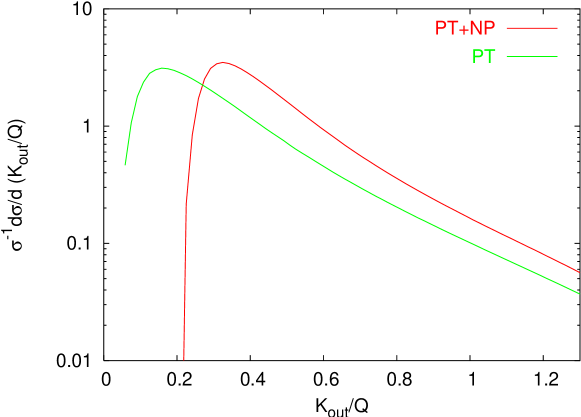
Figure 1: QCD prediction for $x_{\mbox{\scriptsize B}}=0.1$, $Q^{2}=400\mathop{\rm Ge\!V}^{2}$ and $y_{-}=0.1$. In the NP correction we have taken $\alpha_{0}(2\mathop{\rm Ge\!V})=0.52$.

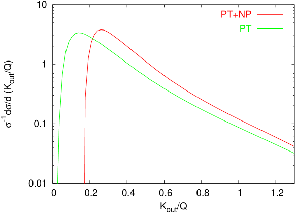
Figure 2: The same as Fig.1 but with $Q^{2}=900\mathop{\rm Ge\!V}^{2}$.

Figs. 1 and 2 show the differential $K_{\mbox{\scriptsize out}}$ distribution for $Q=20\mathop{\rm Ge\!V}$ and $Q=30\mathop{\rm Ge\!V}$, and $x_{\mbox{\scriptsize B}}=0.1$. In order to prevent $T_{M}$ from being too large it is enough to let $y_{+}$ go to its maximum kinematically allowed value $y_{+}=2.5$ (see (62) and (63)). From these pictures one notices the $1/Q$ dependence of the power correction. One can also observe that the shift is larger at smaller $K_{\mbox{\scriptsize out}}$, so that the distribution is squeezed. This is due to the $\ln K_{\mbox{\scriptsize out}}$ dependence of the NP correction (see discussion in section 3.4).

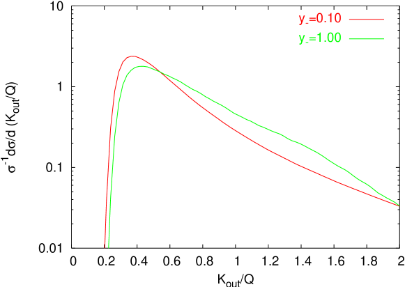
Figure 3: The full (PT+NP) differential $K_{\mbox{\scriptsize out}}$ distribution for two different values of $y_{-}$, for fixed $y_{+}=2.5$, $x_{\mbox{\scriptsize B}}=0.01$ and $Q^{2}=400\mathop{\rm Ge\!V}^{2}$.

The fact that our predictions are also geometry dependent can be seen from Fig. 3, where we plot the PT+NP curve for two different values of $y_{-}$, fixing $y_{+}=2.5$.

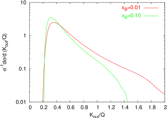
Figure 4: The full (PT+NP) differential $K_{\mbox{\scriptsize out}}$ distribution for two different values of $x_{\mbox{\scriptsize B}}$, for $y_{-}=0.05$, $y_{+}=2.5$, and $Q^{2}=400\mathop{\rm Ge\!V}^{2}$.

Finally, Fig. 4 shows how the distribution depends on the value of $x_{\mbox{\scriptsize B}}$. The distribution dies faster by increasing $x_{\mbox{\scriptsize B}}$. Indeed, for increasing $x_{\mbox{\scriptsize B}}$ the centre-of-mass energy of the hard system decreases, so that the phase space for producing hadrons with large out-of-plane momentum is reduced. Moreover, by increasing $x_{\mbox{\scriptsize B}}$ the configuration with incoming quark or antiquark ($\delta=2,3$) becomes more probable.

5 Discussion and conclusion

In this paper we have extended our knowledge of three-jet physics to the case of a near-to-planar observable in hard electron-proton scattering, defined analogously to the thrust-minor in $e^{+}e^{-}$ annihilation. On the PT side, this observable exhibits a rich colour and geometry dependence. Large angle gluon radiation contributes in setting the relevant scales for the PT radiator (see (35)). The radiator itself is a sum of three contributions, one for each emitting parton, each one characterized by a different hard scale: for a quark or antiquark it is the invariant mass of the fermion system, for a gluon it is its (invariant) transverse momentum with respect to the fermion pair. Such a structure, due to the universality of soft radiation, is found to be common to all near-to-planar $3$-jet shape variables encountered so far (see [10, 11, 12]).

Since the observable $K_{\mbox{\scriptsize out}}$ is uniform in rapidity, hard parton recoil contributes both to the definition of the event plane and to the observable. It contributes then to the PT distribution at SL level.

The thrust major axis is determined only by the hard parton system and cannot be changed (at least at SL accuracy) by secondary soft or collinear parton radiation. This implies that there exists no correlation between the up- and down-regions (see the definition of the event-plane (25)). This property makes the analysis of our observable much simpler than that of the thrust minor $T_{m}$ distribution in $e^{+}e^{-}$. In particular, we are able to write a closed formula for the SL function ${\cal{S}}_{\delta}$ in (38) which embodies the contributions of hard parton recoil.

Our observable exhibits $1/Q$ power corrections arising from the running of the coupling into the infrared region. For $K_{\mbox{\scriptsize out}}\gg\Lambda_{\mbox{\scriptsize QCD}}$ they can be taken into account as a shift of the PT distribution (see (43)). The shift $\delta K_{\mbox{\scriptsize out}}^{(\delta)}$ depends logarithmically on the observable itself, so that the effect of the shift is actually a deformation of the PT distribution. Since $K_{\mbox{\scriptsize out}}$ accumulates contributions from partons of any rapidity, one has to carefully consider effective rapidity cut-off. Along the beam axis the rapidity is bounded by the experimental resolution $\eta_{0}$. Along the direction of the two outgoing hard partons, it is their displacement from the event plane which provides an effective rapidity cut-off. Averaging such a NP correction over the hard parton PT recoil distribution gives rise to contributions of order $\ln K_{\mbox{\scriptsize out}}$ or $1/\sqrt{\alpha_{\mbox{\scriptsize s}}}$ according to the $K_{\mbox{\scriptsize out}}$ régimes. The form of the power corrections can be simply interpreted on the basis of the event plane kinematics (see (25)), as explained in detail in section 3.

As in other $3$-jet observables, the magnitude of the NP shift is expected to be roughly twice as large as the corresponding one for $2$-jet shape variables (the characteristic weight $2C_{F}$ of the DL contribution of the logarithm of $2$-jet distribution becomes here a $2C_{F}+C_{A}$ weight). This implies that higher order power corrections may become important, see [22]. The comparison with data (not yet available) will be needed to check the validity of our method.

Appendix A Kinematics and elementary partonic cross-sections

For the elementary process (15) we may write the parton momenta $P_{1}$, $P_{2}$ as

$$\begin{split}&P_{1}=\frac{Q}{2x}(1,0,0,-1)\>,\quad P_{2}=\frac{Q}{2}(z_{0},0,T_{M},z_{3})\>,\quad\\ &z_{0}=\xi\!+\!\frac{(1\!-\!\xi)(1\!-\!x)}{x}\>,\quad z_{3}=\xi\!-\!\frac{(1\!-\!\xi)(1\!-\!x)}{x}\>,\end{split}$$ (59)

in terms of the variables in (16). Distinguishing $P_{2}$ and $P_{3}$ according to (18), the variable $\xi$ is given in terms of $T_{M}$ by

$$\xi=\frac{1}{2}\left[1-\sqrt{1-\frac{xT_{M}^{2}}{1-x}}\right]\>,$$ (60)

and in terms of $y_{2}$ by the inverse of (19), which is

$$\begin{split}&\xi=\frac{1-x}{2(2x-1)}\left[\sqrt{1+\frac{4x(2x-1)y_{2}}{(1-x)^{2}}}-1\right]\>,\quad\left\{\begin{split}&0<x<\frac{3}{4},\quad 0<y_{2}<\frac{1}{4x}\\ &\frac{3}{4}<x<1,\quad 0<y_{2}<\frac{2(1-x)^{2}}{x(2x-1)}\end{split}\right.\\ &\xi=\frac{x^{2}y_{2}-(1-x)^{2}}{(2x-1)(1-x+xy_{2})}\>,\qquad\qquad\qquad\qquad\>\frac{3}{4}<x<1,\>\frac{2(1-x)^{2}}{x(2x-1)}<y_{2}<\frac{1-x}{x}\end{split}$$ (61)

Note that at any fixed value of $y_{2}$, the freedom to vary $x$ results in events with a range of $T_{M}$ values. If $y_{2}<\frac{1}{3}$, the kinematic upper limit on $x$ is $x=\frac{1}{1+y_{2}}$, at which $\xi=\mbox{\small$\frac{1}{2}$}$ and the lower bound on $T_{M}$ is therefore $\sqrt{y_{2}}$. The lower limit on $x$ is the Bjorken variable $x_{\mbox{\scriptsize B}}$, at which $\xi=\xi(x_{\mbox{\scriptsize B}},y_{2})<x_{\mbox{\scriptsize B}}y_{2}$. (This is obtained by expanding (61) about $x_{\mbox{\scriptsize B}}=0$: the difference from equality is of order $x_{\mbox{\scriptsize B}}^{2}$.) Consequently, $T_{M}<2\sqrt{y_{2}}$. Therefore, restricting ourselves to events in the range (10), with $y_{-}<\frac{1}{3}<y_{+}$, leads to a selection of events whose values of $T_{M}$ lie in the range

$$\sqrt{y_{-}}<T_{M}<2\sqrt{y_{+}}\>.$$ (62)

This of course does not select all events with $T_{M}$ in this range; it is merely a means of selecting events whose $T_{M}$ does not lie outside it, so that we do not need to consider logarithms of $T_{M}$. The phase-space in terms of the variables $(x,\xi)$ then becomes:

$$\begin{split}&x_{\mbox{\scriptsize B}}<x<x_{M}\>,\quad x_{M}=\left\{\begin{split}&\frac{1}{1+y_{-}}\>,\>\>\>y_{-}<1/3\\ &\frac{1}{4y_{-}}\>,\>\>\>\>\>\>\>\>y_{-}>1/3\end{split}\right.\>,\\ &\xi_{-}<\xi<\xi_{+}\>,\quad\xi_{-}=\xi(x,y_{-})\>,\quad\xi_{+}=\left\{\begin{split}&\xi(x,y_{+})\>,\>\>\>x<{\textstyle\frac{1}{4y_{+}}}\\ &\mbox{\small$\frac{1}{2}$}\>,\qquad\quad\>\>x>{\textstyle\frac{1}{4y_{+}}}\end{split}\right..\end{split}$$ (63)

Since we consider only diagrams with the exchange of a single photon or $Z_{0}$, the individual partonic cross-sections may be decomposed according to:

$$\begin{split}\frac{d\hat{\sigma}_{\tau,\delta,f}}{dx\,d\xi\,dQ^{2}}=\frac{\alpha^{2}\alpha_{\mbox{\scriptsize s}}}{Q^{4}}&\Bigl{\{}C^{f}(Q^{2})\left[\left(2-2y+y^{2}\right)C_{T}^{\tau,\delta}(x,\xi)+2(1-y)C_{L}^{\tau,\delta}(x,\xi)\right]\\ &+D^{f}(Q^{2})y(2-y)C_{3}^{\tau,\delta}(x,\xi)\Bigr{\}}\>,\end{split}$$ (64)

into transverse, longitudinal and parity-violating terms. Here $y$ is defined by

$$y=\frac{(Pq)}{(PP_{e})}=\frac{Q^{2}}{x_{\mbox{\scriptsize B}}s}\>,$$ (65)

where $P_{e}$ is the momentum of the incident electron, and $s$ is the centre-of-mass energy squared of the collision (we neglect the proton mass). The flavour-dependent functions $C^{f}(Q^{2})$ and $D^{f}(Q^{2})$ show how the $\gamma$ and $Z$ exchange diagrams combine:

$$\begin{split}C^{f}(Q^{2})&=e_{f}^{2}-\frac{2e_{f}V_{f}V_{e}}{\sin^{2}2\theta_{W}}\left(\frac{Q^{2}}{Q^{2}\!+\!M^{2}}\right)+\frac{(V_{f}^{2}\!+\!A_{f}^{2})(V_{e}^{2}\!+\!A_{e}^{2})}{\sin^{4}2\theta_{W}}\left(\frac{Q^{2}}{Q^{2}\!+\!M^{2}}\right)^{2}\>,\\ D^{f}(Q^{2})&=-\frac{2e_{f}A_{q}A_{e}}{\sin^{2}2\theta_{W}}\left(\frac{Q^{2}}{Q^{2}\!+\!M^{2}}\right)+\frac{4V_{f}A_{f}V_{e}A_{e}}{\sin^{4}2\theta_{W}}\left(\frac{Q^{2}}{Q^{2}\!+\!M^{2}}\right)^{2}.\end{split}$$ (66)

The functions $C_{T/L/3}^{\tau,\delta}(x,\xi)$ are the one loop QCD elementary square matrix elements for the hard vertex (there is no contribution of order ${\cal{O}}\left(\alpha_{\mbox{\scriptsize s}}^{0}\right)$ since we require transverse jets). We have [23]

$$\begin{split}&C_{T}^{q,3}=C_{F}\left[\frac{x^{2}+\xi^{2}}{(1-x)(1-\xi)}+2(1+x\xi)\right]\,,\hskip 11.38092ptC_{T}^{g,1}=\left[x^{2}+(1-x)^{2}\right]\frac{\xi^{2}+(1-\xi)^{2}}{\xi(1-\xi)}\,,\\ &C_{L}^{q,3}=C_{F}\cdot 4x\xi\,,\hskip 136.5733ptC_{L}^{g,1}=8x(1-x)\,,\\ &C_{3}^{q,3}=C_{F}\left[\frac{x^{2}+\xi^{2}}{(1-x)(1-\xi)}+2(x+\xi)\right]\,,\hskip 14.22636ptC_{3}^{g,1}=0\,,\\ &C_{T/L/3}^{q,2}(x,\xi)=C_{T/L/3}^{q,3}(x,1\!-\!\xi)\,,\>\>C_{T/L}^{\bar{q},\delta}(x,\xi)=C_{T/L}^{q,\delta}(x,\xi)\,,\>\>C_{3}^{\bar{q},\delta}(x,\xi)=-C_{3}^{q,\delta}(x,\xi)\,.\end{split}$$ (67)

Appendix B Resumming QCD emission

The QCD results illustrated in section 3 are based on calculations similar to those performed for other $3$-jet shape distributions in $e^{+}e^{-}$ annihilation [10, 11] and in hadronic collisions [12]. Here we follow the method and use the results developed and obtained there. We do not report the full details of the calculations but simply discuss the main features characteristic of the present distribution: for details refer to the later appendices and to the previous papers. In particular here we

• deduce, in the present context, the factorized structure in (27) and identify the hard scale entering the incoming parton distribution ${\cal{P}}$;

• obtain the PT radiation factor at the SL accuracy (33);

• compute the leading order NP corrections giving rise to the shift (43);

• show that, for $K_{\mbox{\scriptsize out}}$ in the range (14), the $\eta_{0}$ dependence enters only in the NP shift.

B.1 Resummation of the distribution

Considering the region $K_{\mbox{\scriptsize out}}\ll Q$, the starting point is the factorization of the square amplitude for the emission of $n$ secondary soft partons in the process (21) (contributions from hard collinear secondary emission are included later). We have

$$|M_{\tau,\delta,f,\,n}(k_{1}\ldots k_{n})|^{2}\simeq|M_{\tau,\delta,f,\,0}|^{2}\cdot S_{\delta,\,n}(k_{1}\ldots k_{n})\>.$$ (68)

The first factor is the Born squared amplitude which gives rise to the elementary hard distribution $d\hat{\sigma}_{\tau,\delta,f}$ in (26). The second factor is the distribution in the soft partons emitted from the system of the three hard partons $p_{1},p_{2}$ and $p_{3}$ in (21). It depends on the colour charges of the emitters which are identified by the configurations $\delta=1,2,3$, the index of the primary gluon momentum. Since soft radiation is universal and does not change the nature of incoming parton, $S_{\delta,\,n}$ does not depend on $\tau$ and $f$. For soft emission, the primary partons $p_{a}$ differ from the hard primary parton momenta $P_{a}$ (depending on $Q,x,\xi$, see Appendix A) by small recoil components.

By using (68), the soft contributions to the cross-section are resummed by

$$\begin{split}\frac{d\sigma(K_{\mbox{\scriptsize out}},y_{\pm})}{dx_{\mbox{\scriptsize B}}\,dQ^{2}}=\sum_{\tau,\delta,f}\int_{x_{\mbox{\scriptsize B}}}^{x_{M}}dx&\int_{\xi_{-}}^{\xi_{+}}d\xi\left(\frac{d\hat{\sigma}_{\tau,\delta,f}}{dx\,d\xi\,dQ^{2}}\right)\int_{0}^{1}dx_{1}{\cal{P}}_{\tau,f}\left(x_{1},\mu\right)\\ &\times\sum_{n}\,\frac{1}{n!}\,\prod_{i=1}^{n}\,\int\frac{d^{3}k_{i}}{\pi\omega_{i}}\>\int d\Phi_{n}\cdot S_{\delta,\,n}\>,\end{split}$$ (69)

with $x_{M}$ given in Appendix A and $x_{1}$ the momentum fraction (22) of the incoming parton and $\mu$ the (small) subtraction scale. The phase space $d\Phi_{n}$ fixes the observable $K_{\mbox{\scriptsize out}}$, the event plane and $x$, the Bjorken variable for the hard elementary distribution $d\hat{\sigma}\,$. The momentum fraction of the parton entering the hard scattering is then

$$\frac{x_{\mbox{\scriptsize B}}}{x}=x_{1}\prod_{i\in{\cal{C}}_{1}}z_{i}\>,$$ (70)

where $z_{i}$ are the collinear splitting fractions for radiation of secondary partons $k_{i}$ in the region ${\cal{C}}_{1}$ collinear to $p_{1}$. The phase space $d\Phi_{n}$ is then given by

$$\begin{split}d\Phi_{n}=&dp_{2x}\,dp_{3x}\,\Theta\left(K_{\mbox{\scriptsize out}}-|p_{2x}|-|p_{3x}|-{\sum_{i}}^{\prime}|k_{ix}|\right)\delta\left(x_{\mbox{\scriptsize B}}\!-\!xx_{1}\prod_{i\in{\cal{C}}_{1}}z_{i}\right)\\ &\delta\left(p_{2x}+{\sum_{i\in U}}^{\prime}k_{ix}+\frac{1}{2}{\sum_{i}}^{\prime\prime}k_{ix}\right)\delta\left(p_{3x}+{\sum_{i\in D}}^{\prime}k_{ix}+\frac{1}{2}{\sum_{i}}^{\prime\prime}k_{ix}\right),\end{split}$$ (71)

where the last two delta functions fix the event plane, as shown in (25).

So the radiation factor ${\cal{I}}$ in (26) takes the form

$${\cal{I}}_{\tau,\delta,f}=x\int_{0}^{1}dx_{1}{\cal{P}}_{\tau,f}\left(x_{1},\mu\right)\>\sum_{n}\,\frac{1}{n!}\,\prod_{i=1}^{n}\,\int\frac{d^{3}k_{i}}{\pi\omega_{i}}\>\int d\Phi_{n}\cdot S_{\delta,\,n}\,.$$ (72)

To resum the secondary parton emissions we use the factorization structure of the soft emission factor $S_{\delta,\,n}$. The phase space $d\Phi_{n}$ can be factorized by Mellin and Fourier transforms. We get

$$\begin{split}&\int d\Phi_{n}=\frac{1}{x_{\mbox{\scriptsize B}}}\int\frac{dN}{2\pi i}\left(\frac{xx_{1}}{x_{\mbox{\scriptsize B}}}\right)^{N-1}\int\frac{d\nu\,e^{\nu K_{\mbox{\scriptsize out}}}}{2\pi i\nu}\\ &\times\prod_{a=2,3}\int_{-\infty}^{\infty}\frac{\nu d\beta_{a}dp_{ax}}{2\pi}e^{-\nu(|p_{ax}|-i\beta_{a}p_{ax})}\prod_{i}\epsilon(z_{i})\,U(k_{i})\,,\end{split}$$ (73)

where

$$\begin{split}\left\{\begin{split}&\epsilon(z)=z^{N-1}\,,\quad\mbox{for}\quad k\in{\cal{C}}_{1}\,,\\ &\epsilon(z)=1\,,\qquad\>\>\>\mbox{for}\quad k\in\!\!\!\!|\>\>{\cal{C}}_{1}\,,\end{split}\right.\end{split}$$ (74)

and

$$\begin{split}\left\{\>\>\begin{split}&U(k)=u_{2}(k_{x})\>\,\equiv e^{-\nu(|k_{x}|-i\beta_{2}k_{x})}\quad\,\mbox{for}\>k_{y}>0\>,\>\>\eta_{k}<\eta_{0}\>,\\ &U(k)=u_{3}(k_{x})\>\,\equiv e^{-\nu(|k_{x}|-i\beta_{3}k_{x})}\quad\,\mbox{for}\>k_{y}<0\>,\>\>\eta_{k}<\eta_{0}\>,\\ &U(k)=u_{0}(k_{x})\>\,\equiv e^{i\frac{\nu}{2}(\beta_{2}+\beta_{3})k_{x}}\qquad\mbox{for}\>\eta_{k}>\eta_{0}\>.\end{split}\right.\end{split}$$ (75)

The last source $u_{0}(k)$ corresponds to partons emitted in the beam region, which contributes only to the momentum conservation and not to the observable $K_{\mbox{\scriptsize out}}$. The near-to-planar region $K_{\mbox{\scriptsize out}}\ll Q$ corresponds to the region $\nu Q\gg 1$ in the Mellin variable.

Resummation can be now performed and one obtains

$$\begin{split}{\cal{I}}_{\tau,\delta,f}(K_{\mbox{\scriptsize out}},x,\xi,Q,x_{\mbox{\scriptsize B}},\eta_{0})&\!=\!\int\frac{d\nu\,e^{\nu K_{\mbox{\scriptsize out}}}}{2\pi i\nu}\!\int_{0}^{1}\frac{dx_{1}}{x_{1}}\int\frac{dN}{2\pi i}\left(\frac{x\,x_{1}}{x_{\mbox{\scriptsize B}}}\right)^{N}{\cal{P}}_{\tau,f}(x_{1},\mu)\\ &\times\prod_{a=2,3}\int\frac{\nu d\beta_{a}dp_{ax}}{2\pi}e^{-\nu(|p_{ax}|-i\beta_{a}p_{ax})}\>e^{-{\cal{E}}_{\delta}}\>,\end{split}$$ (76)

where ${\cal{E}}_{\delta}$ is the full radiator for the secondary emission and is given by

$${\cal{E}}_{\delta}=\int\frac{d^{3}k}{\pi\omega}W_{\delta}(k)\,\left[1-U(k)\epsilon(z)\right]\>.$$ (77)

The $1$ in the brackets here represents virtual gluon emission. The radiator ${\cal{E}}_{\delta}$ depends on the source variables, $\nu,\beta_{a},N,\eta_{0}$, on the primary parton momenta $p_{a}$, which are given in terms of $Q,x,\xi$ and the recoil components $p_{ax}$ (the other components can be neglected in the soft limit), and on the subtraction scale $\mu$ needed to regularize the collinear divergence. Here $W_{\delta}(k)$ is the two-loop distribution for the emission of the soft gluon from the three hard partons $p_{a}$ in the configuration $\delta$:

$$W_{\delta}(k)=\frac{N_{c}}{2}\left(w_{\delta a}(k)+w_{\delta b}(k)-\frac{1}{N_{c}^{2}}w_{ab}(k)\right)\>,\qquad a\neq b\neq\delta\>,$$ (78)

where $w_{ab}(k)$ is the standard distribution for emission of a soft gluon from the $ab$-dipole

$$w_{ab}(k)=\frac{\alpha_{\mbox{\scriptsize s}}(k_{ab,t})}{\pi k_{ab,t}^{2}}\>,\qquad k_{ab,t}^{2}=\frac{2(p_{a}k)(kp_{b})}{(p_{a}p_{b})}\>,$$ (79)

and $\alpha_{\mbox{\scriptsize s}}$ is in the physical scheme [19].

B.2 Factorization of incoming parton distribution

In the present formulation, the factorization (27) of the distribution ${\cal{I}}$ results by splitting the source

$$[1-U(k)\epsilon(z)]=[1-U(k)]\>+\>[1-\epsilon(z)]\,U(k)\>,$$ (80)

so that the radiator ${\cal{E}}$ can be expressed as the sum of two terms (we write explicitly only the $N$ and $\mu$ dependence)

$${\cal{E}}_{\delta}(N,\mu)={\cal{R}}_{\delta}\>+\>\Gamma_{\delta}(N,\mu)\>,$$ (81)

with

$$\begin{split}{\cal{R}}_{\delta}=&\int\frac{d^{3}k}{\pi\omega}\>W_{\delta}(k)\>[1-U(k)]\>,\\ \Gamma_{\delta}(N,\mu)=&\int_{{\cal{C}}_{1}}\frac{d^{3}k}{\pi\omega}\>W_{\delta}(k)\>\left[1-z^{N-1}\right]\,U(k)\>.\end{split}$$ (82)

These two terms will be evaluated for small $K_{\mbox{\scriptsize out}}\sim\nu^{-1}$.

Consider first the collinear singular piece $\Gamma_{\delta}(N,\mu)$. Here the source $U(k)$ provides an upper bound for the integration frequencies of order $\nu^{-1}\sim K_{\mbox{\scriptsize out}}$. This is shown by using, in the integral (82),

$$[1-u_{a}(k_{x})]\>\simeq\>\Theta\left(\,|k_{x}|-\rho_{a}^{-1}\,\right)\>,\qquad\rho_{a}=e^{\gamma_{E}}\nu\sqrt{1+\beta_{a}^{2}}\>,$$ (83)

for $a=2,3$, which is valid for large $\nu$ within SL accuracy (see for instance Appendix C of Ref. [11]). Using this approximate expression one also shows [12] that $\Gamma_{\delta}(N,\nu)$ does not depend on $\eta_{0}$, as long as $K_{\mbox{\scriptsize out}}$ is taken in the range (14). As shown in [12], $\Gamma(N,\nu)$ is the soft part of the anomalous dimension that evolves the parton distributions ${\cal{P}}$ from the small subtraction scale to the scale $\rho_{a}^{-1}$. It is accurate at two loop order provided we use the coupling in the physical scheme [19], and it is diagonal in the configuration index since soft radiation is universal and does not change the nature of the incoming parton. But in general one needs the full anomalous dimension (including the hard non diagonal pieces) so that the incoming partons may change from a quark to a gluon and vice versa. The resulting exponent $\Gamma$ becomes a matrix. Upon integration over $x_{1}$ and the Mellin variable $N$

$$\int_{0}^{1}\frac{dx_{1}}{x_{1}}\int\frac{dN}{2\pi i}\left(\frac{x\,x_{1}}{x_{\mbox{\scriptsize B}}}\right)^{N}\!{\cal{P}}(x_{1},\mu)\cdot e^{-\Gamma(N,\mu)}\,\simeq\,{\cal{P}}\left(\frac{x_{\mbox{\scriptsize B}}}{x},K_{\mbox{\scriptsize out}}\right)\>,$$ (84)

one obtains the parton distribution ${\cal{P}}(K_{\mbox{\scriptsize out}})$ evolved from the subtraction to the hard scale $K_{\mbox{\scriptsize out}}$, up to terms that are beyond SL. The $\mu$ dependence in ${\cal{P}}(\mu)$ and $\Gamma(N,\mu)$ is cancelled. We do not consider here power corrections since they are of second order ($1/Q^{2}$), see [4].

We consider then the piece ${\cal{R}}_{\delta}$. This is a CIS quantity ($[1\!-\!U(k)]\!\to\!0$ for $k_{t}\!\to\!0$) which produces the radiation factor ${\cal{A}}_{\delta}$ in (27)

$${\cal{A}}_{\delta}(K_{\mbox{\scriptsize out}},x,\xi,Q,\eta_{0})=\int\frac{d\nu\,e^{\nu K_{\mbox{\scriptsize out}}}}{2\pi i\nu}\,\hat{{\cal{A}}}_{\delta}(\nu,x,\xi,Q,\eta_{0})\>,$$ (85)

with the Mellin moment

$$\hat{{\cal{A}}}_{\delta}=\int\prod_{a=2,3}\frac{\nu d\beta_{a}dp_{ax}}{2\pi}\,e^{-\nu(|p_{ax}|-i\beta_{a}p_{ax})}\>e^{-{\cal{R}}_{\delta}}\>.$$ (86)

All the PT contributions are finite and they can be evaluated to SL accuracy by using the approximation (83) for the sources. The PT resummed expression ${\cal{R}}^{\mbox{\scriptsize PT}}_{\delta}$ is then obtained by evaluating the integral (82) of ${\cal{R}}_{\delta}$ using (83).

However the virtual momentum $k_{t}$, entering the SL resummed running coupling in ${\cal{R}}_{\delta}$, cannot be prevented from going to zero. Although the contribution from this NP region is (formally) highly subleading (power suppressed), it is phenomenologically quite important for $K_{\mbox{\scriptsize out}}$ not too large [3]. For $k_{t}$ very small (in particular for $|k_{x}|\ll\nu^{-1}\sim K_{\mbox{\scriptsize out}}$) the approximation (83) is no longer valid and we have instead

$$[1-u_{a}(k)]\simeq\nu\,(|k_{x}|-i\beta_{a}k_{x})\>,$$ (87)

so that the leading NP correction to ${\cal{R}}_{\delta}$ is

$$\delta{\cal{R}}_{\delta}\simeq\nu\cdot\delta K_{\mbox{\scriptsize out}}^{(\delta)}\>,$$ (88)

corresponding to a shift in $K_{\mbox{\scriptsize out}}$ in (85). To evaluate this NP shift we use the dispersive method [4] to represent the running coupling and we evaluate the leading power-suppressed contribution from (87).

The two contributions to the radiator

$${\cal{R}}_{\delta}={\cal{R}}^{\mbox{\scriptsize PT}}_{\delta}+\delta{\cal{R}}_{\delta}\>,$$ (89)

together with the expression for the radiation factor ${\cal{A}}_{\delta}$ will be described in the next two subsections.

B.3 PT Radiation Factor

The PT radiator ${\cal{R}}_{\delta}^{\mbox{\scriptsize PT}}$ to SL accuracy coincides with a particular case of the PT radiator computed for $T_{m}$ in $e^{+}e^{-}$ annihilation (where we set $\gamma=\beta_{1}=0$ in eq. (4.8) of Ref. [10]). For $K_{\mbox{\scriptsize out}}$ in the range (14) this contribution is $\eta_{0}$ independent, see [12]. The explicit calculation is given in Appendix C, and the result may be conveniently separated into two terms:

$${\cal{R}}_{\delta}^{\mbox{\scriptsize PT}}=R_{12}^{(\delta)}(\rho_{2})+R_{13}^{(\delta)}(\rho_{3})\>,$$ (90)

where

$$R_{1a}^{(\delta)}(\rho_{a})=\mbox{\small$\frac{1}{2}$}C_{1}^{(\delta)}r(\rho_{a},\zeta_{1}^{(\delta)}Q_{1}^{(\delta)})+C_{a}^{(\delta)}r(\rho_{a},\zeta_{a}^{(\delta)}Q_{a}^{(\delta)})\>,$$ (91)

with the function $r$ given in (36) and colour charges $C_{a}^{(\delta)}$ and hard scales $Q_{a}^{(\delta)}$ given in (35). The term $R_{12}^{(\delta)}$ corresponds to the emission in the up-region off parton $p_{1}$ and $p_{2}$. Similarly for $R_{13}^{(\delta)}$. For the PT evaluation we can expand to SL accuracy

$$\begin{split}{\cal{R}}_{\delta}^{\mbox{\scriptsize PT}}=R_{\delta}\left(\nu,x,\xi,Q\right)+\left(C_{T}\gamma_{E}+C_{12}^{(\delta)}\ln\sqrt{1\!+\!\beta_{2}^{2}}+C_{13}^{(\delta)}\ln\sqrt{1\!+\!\beta_{3}^{2}}\right)r^{\prime}(\nu,Q)\,,\end{split}$$ (92)

with $R_{\delta}$ the DL exponent function introduced in (34) and $r^{\prime}$ the SL function (37). Since the radiator is independent of the recoils we can integrate over $p_{ax}$ and, using the expansion (92), we obtain the Mellin moment

$$\begin{split}\hat{{\cal{A}}}^{\mbox{\scriptsize PT}}_{\delta}&(\nu,x,\xi,Q)=\prod_{a=2,3}\int_{-\infty}^{\infty}\frac{d\beta_{a}}{\pi(1+\beta_{a}^{2})}e^{-R^{(\delta)}_{1a}}\\ &\simeq e^{-R_{\delta}\left(\nu,x,\xi,Q\right)}\,e^{-\gamma_{E}C_{T}\,r^{\prime}}{\cal{F}}\left(C_{12}^{(\delta)}\,r^{\prime}\right){\cal{F}}\left(C_{13}^{(\delta)}\,r^{\prime}\right),\qquad r^{\prime}=r^{\prime}(\nu,Q)\>,\end{split}$$ (93)

with ${\cal{F}}$ given in (39).

The PT radiation factor is obtained by integrating over the Mellin variable $\nu$. We make use of the operator identity

$$\int\frac{d\nu\,e^{\nu K_{\mbox{\scriptsize out}}}}{2\pi i\nu}\>G(\nu)=\frac{1}{\Gamma\left(1+\frac{\partial}{\partial\ln K_{\mbox{\scriptsize out}}}\right)}\>G(K_{\mbox{\scriptsize out}}^{-1})$$ (94)

for any logarithmically varying function $G$. (To prove this, multiply both sides by the $\Gamma$-function operator and use the definition $\Gamma(z)=\int_{0}^{\infty}dx\,x^{z-1}e^{-x}$.) Thus to SL accuracy we have

$${\cal{A}}^{\mbox{\scriptsize PT}}_{\delta}(K_{\mbox{\scriptsize out}},x,\xi,Q)=\frac{\hat{{\cal{A}}}^{\mbox{\scriptsize PT}}_{\delta}(K_{\mbox{\scriptsize out}}^{-1},x,\xi,Q)}{\Gamma\left(1+C_{T}r^{\prime}(K_{\mbox{\scriptsize out}}^{-1},Q)\right)}\>,$$ (95)

which corresponds to the PT result in (33), (36) and (38).

B.4 Radiation Factor including NP corrections

The NP correction to the radiator is computed in Appendix D following the standard procedure (see [10]): we assume that the running coupling can be defined even at small momenta via a dispersion relation [4], and we take into account the non-inclusiveness of the observable via the Milan factor. The NP correction is proportional to the parameter $\lambda^{\mbox{\scriptsize NP}}$, given in (134), expressed in terms of the integral of the running coupling in the small momentum region. This parameter takes into account merging of NP and PT corrections at two loops and is the same as entering all the jet-shape distributions so far studied. We obtain

$$\delta{\cal{R}}_{\delta}=\nu\lambda^{\mbox{\scriptsize NP}}\left(C_{1}^{(\delta)}\ln\frac{xe^{\eta_{0}}Q_{1}^{(\delta)}}{Q}+\sum_{a=2,3}C_{a}^{(\delta)}\ln\frac{\zeta Q_{a}^{(\delta)}}{|p_{ax}|}\right)\>,\qquad\zeta=2e^{-2}\>,$$ (96)

where $Q_{a}^{(\delta)}$ are the scales introduced in (35). The NP radiator is made up of three contributions, one for each emitting parton. The hard scales are determined by large angle NP gluons; they are therefore the same as in the PT case. What makes the difference between the three contributions is the NP gluon rapidity cutoff. Actually, when a NP gluon is emitted from the incoming parton $p_{1}$, its rapidity is bounded by the experimental resolution $\eta_{0}$. This is not the case for the emission from $p_{2}$ or $p_{3}$, where it is the out-of-plane momentum of the recoiling parton which provides an effective rapidity cutoff.

The first order NP correction to the Mellin moment $\hat{\cal{A}}_{\delta}$ in (86) is given by

$$\hat{\cal{A}}_{\delta}(\nu)=\prod_{a=2,3}\int\frac{\nu d\beta_{a}dp_{3x}}{2\pi}\,e^{-\nu(|p_{ax}|-i\beta_{a}p_{ax})}\>e^{-R^{\mbox{\scriptsize PT}}_{\delta}}\,\left\{1-\delta{\cal{R}}_{\delta}\right\}\>,$$ (97)

where $R^{\mbox{\scriptsize PT}}_{\delta}$ is the PT radiator in (90). The first term yields the PT contribution in (33) and so we can write

$$\hat{\cal{A}}_{\delta}(\nu)=\hat{\cal{A}}_{\delta}^{\mbox{\scriptsize PT}}(\nu)-\nu\,\lambda^{\mbox{\scriptsize NP}}\>f_{\delta}(\nu)\>.$$ (98)

After the $p_{ax}$ integration the NP correction is given by

$$f_{\delta}(\nu)\!=\!\prod_{a=2,3}\!\int_{-\infty}^{\infty}\!\!\frac{d\beta_{a}}{\pi(1\!+\!\beta_{a}^{2})}\,e^{-{\cal{R}}_{\delta}^{\mbox{\scriptsize PT}}}\!\!\left(\!C_{1}^{(\delta)}\ln\frac{xe^{\eta_{0}}Q_{1}^{(\delta)}}{Q}\!+\!\sum_{a=2,3}\!C_{a}^{(\delta)}[\ln\zeta\,\bar{\nu}\,Q_{a}^{(\delta)}\!+\!\chi(\beta_{a})]\!\right),$$ (99)

with $\chi(\beta)=\ln\sqrt{1+\beta^{2}}+\beta\tan^{-1}\beta$. This function is growing as $\pi|\beta|/2$ at large $\beta$. As a consequence, the $\beta_{a}$ integration in (99) is no longer fastly convergent and we cannot expand the PT radiator as in (92) but we need to keep its exact expression. The region of large $|\beta_{a}|$, which corresponds to $|p_{ax}|\ll K_{\mbox{\scriptsize out}}$, gives the leading NP correction.

The radiation factor ${\cal{A}}$ is obtained by performing the $\nu$ integration so that

$${\cal{A}}_{\delta}(K_{\mbox{\scriptsize out}})={\cal{A}}_{\delta}^{\mbox{\scriptsize PT}}(K_{\mbox{\scriptsize out}})+\delta{\cal{A}}_{\delta}(K_{\mbox{\scriptsize out}})\>.$$ (100)

In Appendix E, see also [7, 10], we show that $\delta{\cal{A}}_{\delta}$ can be expressed (to first order) as a shift (see (43))

$$\delta{\cal{A}}_{\delta}(K_{\mbox{\scriptsize out}})=-\lambda^{\mbox{\scriptsize NP}}\partial_{K_{\mbox{\scriptsize out}}}\int\frac{d\nu\,e^{\nu K_{\mbox{\scriptsize out}}}}{2\pi i\nu}\,f_{\delta}(\nu)\simeq-\delta K_{\mbox{\scriptsize out}}^{(\delta)}\cdot\partial_{K_{\mbox{\scriptsize out}}}{\cal{A}}_{\delta}^{\mbox{\scriptsize PT}}(K_{\mbox{\scriptsize out}})\>,$$ (101)

where the shift is given by

$$\begin{split}&\frac{\delta K_{\mbox{\scriptsize out}}^{(\delta)}}{\lambda^{\mbox{\scriptsize NP}}}=C_{1}^{(\delta)}\ln\frac{xe^{\eta_{0}}Q_{1}^{(\delta)}}{Q}\!+\!\sum_{a=2,3}C_{a}^{(\delta)}\!\left[\ln\frac{Q_{a}^{(\delta,\mbox{\scriptsize NP})}}{2\bar{K}_{\mbox{\scriptsize out}}}+\frac{C_{T}\!-\!C_{1a}^{(\delta)}}{C_{T}}\left\{E_{a}^{(\delta)}(\bar{K}_{\mbox{\scriptsize out}}^{-1})\!+\!{\cal{C}}_{a}^{(\delta)}\right\}\right].\end{split}$$ (102)

Here the NP hard scale is defined by

$$\begin{split}\ln\frac{Q_{a}^{(\delta,\mbox{\scriptsize NP})}}{2\bar{K}_{\mbox{\scriptsize out}}}&=\ln\frac{\zeta Q_{a}^{(\delta)}}{\bar{K}_{\mbox{\scriptsize out}}}+\psi(1+C_{T}\,r^{\prime})+\mbox{\small$\frac{1}{2}$}\psi\left(1\!+\!\frac{C_{1a}^{(\delta)}\,r^{\prime}}{2}\right)-\mbox{\small$\frac{1}{2}$}\psi\left(\frac{1\!+\!C_{1a}^{(\delta)}\,r^{\prime}}{2}\right)\\ &\simeq\ln\frac{2\,\zeta Q_{a}^{(\delta)}}{K_{\mbox{\scriptsize out}}}+{\cal{O}}\left(r^{\prime}\right)\>,\quad\bar{K}_{\mbox{\scriptsize out}}=e^{-\gamma_{E}}K_{\mbox{\scriptsize out}}\>,\end{split}$$ (103)

where $r^{\prime}=r^{\prime}(K_{\mbox{\scriptsize out}}^{-1},Q)$ and the choice of factors of 2 and $e^{-\gamma_{E}}$ is so as to give the simple form for equation (109) below. The function $E_{a}^{(\delta)}$ is given by

$$\begin{split}E_{a}^{(\delta)}(\bar{K}_{\mbox{\scriptsize out}}^{-1})=\int_{\bar{K}_{\mbox{\scriptsize out}}^{-1}}^{\infty}\frac{d\rho}{\rho}e^{-R_{1a}^{(\delta)}(\rho)+R^{(\delta)}_{1a}(\bar{K}_{\mbox{\scriptsize out}}^{-1})}\left(\frac{{\cal{P}}(\rho_{a}^{-1})}{{\cal{P}}(K_{\mbox{\scriptsize out}})}\right)^{\frac{1}{2}}\>,\end{split}$$ (104)

where the appearence of the parton distributions comes from the mismatch between the correct scales $\rho_{a}^{-1}$ and the SL approximation $K_{\mbox{\scriptsize out}}$ in (84). They introduce a dependence on $\tau,\>f$ and $x_{\mbox{\scriptsize B}}$ which we suppress.

As explained in detail in [10], these functions result from an interplay between PT and NP contributions. They can be expressed as the average of the rapidity length over the Sudakov factor for emitting in the up- or down-region for $a=2$ or $a=3$ respectively. Finally,

$${\cal{C}}_{a}^{(\delta)}=\left(E_{a}^{(\delta)}(\bar{K}_{\mbox{\scriptsize out}}^{-1})-\frac{1}{C_{1a}^{(\delta)}r^{\prime}}\right)\left(\frac{1}{{\cal{F}}\left(C_{1a}^{(\delta)}r^{\prime}\right)}-1\right)$$ (105)

is a regular function of $r^{\prime}$.

The shift can be expressed as a sum of partial shifts as in (44) with the rapidity integrals given by

$$\begin{split}&Y_{21}^{(\delta)}=Y_{31}^{(\delta)}=\ln\frac{xe^{\eta_{0}}Q_{1}^{(\delta)}}{Q}\,,\\ &Y_{22}^{(\delta)}=\ln\frac{Q_{2}^{(\delta,\mbox{\scriptsize NP})}}{2\bar{K}_{\mbox{\scriptsize out}}}\,,\qquad\qquad\>\>\>\>Y_{33}^{(\delta)}=\ln\frac{Q_{3}^{(\delta,\mbox{\scriptsize NP})}}{2\bar{K}_{\mbox{\scriptsize out}}}\,,\\ &Y_{23}^{(\delta)}=L_{3}^{(\delta)}(\bar{K}_{\mbox{\scriptsize out}})+{\cal{C}}_{3}^{(\delta)}\,,\qquad Y_{32}^{(\delta)}=L_{2}^{(\delta)}(\bar{K}_{\mbox{\scriptsize out}})+{\cal{C}}_{2}^{(\delta)}\>,\end{split}$$ (106)

where we have introduced the NP functions $L_{a}$ defined as

$$\begin{split}L^{(\delta)}_{a}(\bar{K}_{\mbox{\scriptsize out}})=\ln\frac{Q_{a}^{(\delta,\mbox{\scriptsize NP})}}{2\bar{K}_{\mbox{\scriptsize out}}}+E^{(\delta)}_{a}(\bar{K}_{\mbox{\scriptsize out}}^{-1})\>.\end{split}$$ (107)

These functions have the following asymptotic expansions: from (159) one has

$$L^{(\delta)}_{a}(\bar{K}_{\mbox{\scriptsize out}})=\ln\frac{Q_{a}^{(\delta,\mbox{\scriptsize NP})}}{2\bar{K}_{\mbox{\scriptsize out}}}\left\{1+{\cal{O}}\left(\frac{1}{\alpha_{\mbox{\scriptsize s}}\ln^{2}\frac{Q}{K_{\mbox{\scriptsize out}}}}\right)\right\}\>,\qquad\alpha_{\mbox{\scriptsize s}}\ln^{2}\frac{Q}{K_{\mbox{\scriptsize out}}}\gg 1\>,$$ (108)

while from (160) one obtains the behaviour of $L_{a}$ in the region $\alpha_{\mbox{\scriptsize s}}\ln^{2}Q/K_{\mbox{\scriptsize out}}\ll 1$:

$$\begin{split}L^{(\delta)}_{a}(\bar{K}_{\mbox{\scriptsize out}})=\frac{\pi}{2\sqrt{C^{(\delta)}_{1a}\,\alpha_{\mbox{\scriptsize s}}}}&-\frac{1}{C^{(\delta)}_{1a}}\left(\!\mbox{\small$\frac{1}{2}$}C^{(\delta)}_{1}\ln\frac{Q_{1}^{(\delta,\mbox{\scriptsize PT})}}{Q_{a}^{(\delta,\mbox{\scriptsize NP})}}+C^{(\delta)}_{a}\ln\frac{Q_{a}^{(\delta,\mbox{\scriptsize PT})}}{Q_{a}^{(\delta,\mbox{\scriptsize NP})}}\right.\\ &\left.+\frac{\pi}{4\alpha_{\mbox{\scriptsize s}}}\frac{\partial\ln{\cal{P}}(K_{\mbox{\scriptsize out}})}{\partial\ln K_{\mbox{\scriptsize out}}}+\frac{\beta_{0}}{6}\!\right)\!+\!{\cal{O}}\left(\sqrt{\alpha_{\mbox{\scriptsize s}}}\right),\end{split}$$ (109)

where the PT hard scale is $Q_{a}^{(\delta,\mbox{\scriptsize PT})}=\zeta_{a}^{(\delta)}Q_{a}^{(\delta)}$.

Appendix C The PT radiator

The PT radiator is given, to SL accuracy, in terms of $ab$-dipole radiators

$$r_{ab}(\nu,\beta_{2},\beta_{3})=r_{ab}^{U}(\nu,\beta_{2})+r_{ab}^{D}(\nu,\beta_{3})\>,$$ (110)

where the ‘up’ and ‘down’ hemisphere components are given by

$$\begin{split}r_{ab}^{U}(\nu,\beta_{2})&=\int_{k_{y}>0}\frac{d^{3}k}{\pi\omega}w_{ab}(k)\,\left[1-e^{-\nu(|k_{x}|-i\beta_{2}k_{x})}\right],\qquad w_{ab}(k)=\frac{\alpha_{\mbox{\scriptsize s}}(k^{2}_{ab,t})}{\pi k^{2}_{ab,t}}\>,\\ r_{ab}^{D}(\nu,\beta_{3})&=\int_{k_{y}<0}\frac{d^{3}k}{\pi\omega}w_{ab}(k)\,\left[1-e^{-\nu(|k_{x}|-i\beta_{3}k_{x})}\right],\end{split}$$ (111)

and $k_{ab,\,t}$ is the invariant transverse momentum of $k$ with respect to the $P_{a},P_{b}$ hard partons in (59). For the configuration $\delta=1$, for instance, we have

$$R^{\mbox{\scriptsize PT}}_{1}(\nu,\beta_{a})=\frac{N_{c}}{2}\left(r_{12}(\nu,\beta_{a})+r_{13}(\nu,\beta_{a})-\frac{1}{N_{c}^{2}}\,r_{23}(\nu,\beta_{a})\right).$$ (112)

To evaluate the $ab$-dipole radiator $r_{ab}(\nu,\beta_{a})$ we work in the centre of mass system of the $ab$-dipole. We neglect the rapidity cut (6): the correction is beyond our accuracy [12]. Denoting by $P^{*}_{a},P^{*}_{b}$ and $k^{*}$ the momenta in this system, we introduce the Sudakov decomposition

$$P_{a}^{*}=\frac{Q_{ab}}{2}(1,0,0,1)\>,\quad P_{b}^{*}=\frac{Q_{ab}}{2}(1,0,0,-1)\>,\qquad k^{*}=\alpha P_{a}^{*}+\beta P_{b}^{*}+\kappa\>,$$ (113)

where the scales $Q_{ab}^{2}=2(P_{a}P_{b})$ are given in (17). Here the two-dimensional vector $\vec{\kappa}$ is the transverse momentum orthogonal to the $ab$-dipole momenta ($\kappa^{2}=k^{2}_{ab,t}$). We have then

$$w_{ab}(k)=\frac{\alpha_{\mbox{\scriptsize s}}(\kappa^{2})}{\pi\kappa^{2}}\>,\qquad\frac{d^{3}k}{\pi\omega}=\frac{d^{2}\kappa}{\pi}\frac{d\alpha}{\alpha}\>,\quad\alpha>\frac{\kappa^{2}}{Q^{2}_{ab}}\>.$$ (114)

Since, neglecting the recoils, the outgoing momenta $P_{2}$ and $P_{3}$ are in the $yz$-plane, the Lorentz transformation is in the $yz$-plane and our observable $k_{x}$ remains unchanged. However, the boundary between the ‘up’ and ‘down’ hemispheres becomes non-trivial, and different for each dipole, so we must take each in turn.

The $12$-radiator with

$$k^{*}=\alpha P_{2}^{*}+\beta P_{1}^{*}+\kappa\>,$$ (115)

has up and down hemispheres given by

$$U\>:\kappa_{y}>-\frac{QT_{M}}{2}\alpha\>,\qquad D\>:\kappa_{y}<-\frac{QT_{M}}{2}\alpha\>,$$ (116)

with $T_{M}$ related to $\xi$ by (60). The up component is then

$$r_{12}^{U}(\nu,\beta_{2})=\int_{0}^{Q^{2}_{12}}\frac{d^{2}\kappa}{\pi\kappa^{2}}\frac{\alpha_{\mbox{\scriptsize s}}(\kappa)}{\pi}\int_{\kappa^{2}/Q_{12}^{2}}^{1}\frac{d\alpha}{\alpha}\left[1-e^{-\nu(|\kappa_{x}|-i\beta_{2}\kappa_{x})}\right]\Theta\left(\alpha+\frac{2\kappa_{y}}{QT_{M}}\right)\>,$$ (117)

Integrating over $\alpha$ and $\kappa_{y}$ we have

$$r_{12}^{U}(\nu,\beta_{2})=\int_{-Q_{12}}^{Q_{12}}\frac{dk_{x}}{|k_{x}|}\left[1-e^{-\nu(|k_{x}|-i\beta_{2}k_{x})}\right]\cdot\frac{\alpha_{\mbox{\scriptsize s}}(2|k_{x}|)}{\pi}\left(\ln\frac{Q_{12}}{2|k_{x}|}+\frac{1}{2}\ln\frac{QT_{M}}{2|k_{x}|}\right)\>.$$ (118)

To show this we introduced $\kappa_{y}=t\cdot|k_{x}|$ and used

$$\int_{-\infty}^{\infty}\frac{dt}{\pi(1+t^{2})}\alpha_{\mbox{\scriptsize s}}\left(|k_{x}|\sqrt{1+t^{2}}\right)\ln\frac{Q_{ab}}{|k_{x}|\sqrt{1+t^{2}}}\simeq\alpha_{\mbox{\scriptsize s}}(2|k_{x}|)\ln\frac{Q_{ab}}{2|k_{x}|}\>.$$ (119)

We extended the $t$-integration to infinity since it is convergent, then we integrated over $t$ by expanding $\alpha_{\mbox{\scriptsize s}}$ to second order. Corrections are beyond SL accuracy.

Finally, using (83), we obtain

$$r_{12}^{U}(\nu,\beta_{2})=2\int_{\rho_{2}^{-1}}^{Q_{12}}\frac{dk_{x}}{k_{x}}\frac{\alpha_{\mbox{\scriptsize s}}(2k_{x})}{\pi}\>\left(\ln\frac{Q_{12}}{2k_{x}}+\frac{1}{2}\ln\frac{QT_{M}}{2k_{x}}\right)\>.$$ (120)

Similarly the ‘down’ hemisphere contribution is

$$r_{12}^{D}(\nu,\beta_{3})=2\int_{\rho_{3}^{-1}}^{Q_{12}}\frac{dk_{x}}{k_{x}}\frac{\alpha_{\mbox{\scriptsize s}}(2k_{x})}{\pi}\>\left(\ln\frac{Q_{12}}{2k_{x}}-\frac{1}{2}\ln\frac{QT_{M}}{2k_{x}}\right)\>.$$ (121)

The $13$ radiator has analogous results

$$\begin{split}r_{13}^{U}(\nu,\beta_{2})&=2\int_{\rho_{2}^{-1}}^{Q_{13}}\frac{dk_{x}}{k_{x}}\frac{\alpha_{\mbox{\scriptsize s}}(2k_{x})}{\pi}\>\left(\ln\frac{Q_{13}}{2k_{x}}-\frac{1}{2}\ln\frac{QT_{M}}{2k_{x}}\right)\>,\\ r_{13}^{D}(\nu,\beta_{3})&=2\int_{\rho_{3}^{-1}}^{Q_{13}}\frac{dk_{x}}{k_{x}}\frac{\alpha_{\mbox{\scriptsize s}}(2k_{x})}{\pi}\>\left(\ln\frac{Q_{13}}{2k_{x}}+\frac{1}{2}\ln\frac{QT_{M}}{2k_{x}}\right)\>.\end{split}$$ (122)

The $23$-radiator has a slightly different structure: with

$$k^{*}=\alpha P_{2}^{*}+\beta P_{3}^{*}+\kappa\>,$$ (123)

the up and down hemispheres are given by

$$U\>:\kappa_{y}>\frac{QT_{M}}{2}\frac{\beta-\alpha}{1-2\xi}\>,\qquad D\>:\kappa_{y}<\frac{QT_{M}}{2}\frac{\beta-\alpha}{1-2\xi}\>.$$ (124)

The up component is then

$$\begin{split}r_{23}^{U}(\nu,\beta_{2})=\int_{0}^{Q^{2}_{23}}&\frac{d^{2}\kappa}{\pi\kappa^{2}}\frac{\alpha_{\mbox{\scriptsize s}}(\kappa)}{\pi}\int_{\kappa^{2}/Q_{23}^{2}}^{1}\frac{d\alpha}{\alpha}\left[1-e^{-\nu(|\kappa_{x}|-i\beta_{2}\kappa_{x})}\right]\\ &\Theta\left(\alpha-\frac{\kappa_{y}(1-2\xi)}{QT_{M}}-\sqrt{\frac{\kappa_{y}^{2}}{Q^{2}T_{M}^{2}}+\frac{\kappa_{x}^{2}}{Q_{23}^{2}}}\right)\>,\end{split}$$ (125)

Performing the integrals as above we obtain

$$r_{23}^{U}(\nu,\beta_{2})=2\int_{\rho_{2}^{-1}}^{Q_{23}}\frac{dk_{x}}{k_{x}}\frac{\alpha_{\mbox{\scriptsize s}}(2k_{x})}{\pi}\ln\frac{Q_{23}}{2k_{x}}\>,$$ (126)

and similarly

$$r_{23}^{D}(\nu,\beta_{3})=2\int_{\rho_{3}^{-1}}^{Q_{23}}\frac{dk_{x}}{k_{x}}\frac{\alpha_{\mbox{\scriptsize s}}(2k_{x})}{\pi}\ln\frac{Q_{23}}{2k_{x}}\>.$$ (127)

Assembling the various dipole contributions and including hard collinear splittings then yields, to SL accuracy,

$$\begin{split}R_{\delta}^{\mbox{\scriptsize PT}}(\nu,\beta_{2},\beta_{3})=\frac{1}{2}&\sum_{a=1}^{3}C_{a}^{(\delta)}\left[r(\rho_{2},\zeta_{a}^{(\delta)}Q_{a}^{(\delta)})+r(\rho_{3},\zeta_{a}^{(\delta)}Q_{a}^{(\delta)})\right]\\ &+\frac{1}{2}\left(C_{2}^{(\delta)}-C_{3}^{(\delta)}\right)\left[r(\rho_{2},QT_{M})-r(\rho_{3},QT_{M})\right]\>.\end{split}$$ (128)

Finally, we note that the terms on the second line contribute only at SL level, since the DL terms cancel. We may therefore change at will the hard scales in these terms, yielding the result (90).

Appendix D NP corrections to the radiator

We consider the NP correction $\delta r_{ab}$ to the $ab$-dipole radiator. In this case, as we shall see, we need to retain both the recoil momenta $p_{2x}$ and $p_{3x}$ and the rapidity cut $\eta_{0}$ . We write the integral in the $ab$-dipole centre of mass variables $\alpha,\beta$ and $\vec{\kappa}$ introduced in (113) and, to obtain the NP correction $\delta r_{ab}$, we perform the following standard operations:

• the running coupling, reconstructed by two loop emission, is represented by the dispersive form [4]. Then, the $ab$-dipole radiation $w_{ab}(k)$ is written in the $ab$-centre of mass system (see (114)) in the form

  $$w_{ab}(k)=\frac{\alpha_{\mbox{\scriptsize s}}(\kappa)}{\pi\kappa^{2}}=\int_{0}^{\infty}\frac{dm^{2}\,\alpha_{\mbox{\scriptsize eff}}(m)}{\pi(\kappa^{2}+m^{2})^{2}}\>;$$ (129)

• to take into account the emission of soft partons at two loop order [6], we need to extend the source $u(k_{x})$ to include the mass $m$ of the soft system. We assume $k_{x}=\kappa\cos\phi\to\sqrt{\kappa^{2}+m^{2}}\cos\phi$, with $\phi$ the azimuthal angle of $\vec{\kappa}$. Similarly we introduce the mass in the kinematical relations such as $\alpha\beta=(\kappa^{2}+m^{2})/Q_{ab}^{2}$ for the $ab$-dipole variables;

• we take the NP part $\delta\alpha_{\mbox{\scriptsize eff}}(m)$ of the effective coupling. Since it has support only for small $m$, we take the leading part of the integrand for small $\kappa$, and $m$. In particular we linearize the source $U(k)$

  $$\left[1-U(k)\right]\>\to\>\nu\sqrt{\kappa^{2}+m^{2}}\>|\cos\phi|\>\Theta(\eta_{0}-\eta_{k})\>.$$ (130)

  Recall that $\eta_{k}$ is the rapidity of $k$ in the Breit frame (4). Here we have neglected terms proportional to $\beta_{2}$ and $\beta_{3}$ since they vanish, by symmetry, upon the $\beta_{a}$ integration;

• the recoil component $p_{ax}$ of the outgoing parton $p_{a}$ does provide an effective cut in the soft gluon rapidity along the outgoing parton [10, 7]. This is due to a real-virtual cancellation which takes place when the angle of the outgoing parton $p_{a}$ with the event plane exceeds the corresponding angle of the soft gluon. The detailed analysis of real and virtual pieces entails that the contribution from the observable $\sqrt{\kappa^{2}+m^{2}}\>|\cos\phi|$ in the linear expansion of the source (see (130)) has to be replaced by

  $$\sqrt{\kappa^{2}+m^{2}}\>|\cos\phi|\to\left|\sqrt{\kappa^{2}+m^{2}}\,\cos\phi+\alpha p_{ax}\right|-\alpha|p_{ax}|\>,$$ (131)

  with $\alpha$ the Sudakov variable in the $ab$-dipole centre of mass in the forward region $\alpha>\beta$;

• to take fully into account effects of non-inclusiveness of jet observables at two-loop order, we multiply the radiator by the Milan factor [6, 16]

  $${\cal{M}}=\frac{3}{64}\frac{(128\pi+128\pi\ln 2-35\pi^{2})C_{A}-5\pi^{2}n_{f}}{11C_{A}-2n_{f}}\>,$$ (132)

  using $n_{f}=3$;

• the NP correction is finally expressed in terms of the parameter

  $$\lambda^{\mbox{\scriptsize NP}}=2{\cal{M}}\,c_{K_{\mbox{\scriptsize out}}}\int dm\frac{\delta\alpha_{\mbox{\scriptsize eff}}(m)}{\pi}\>,\quad c_{K_{\mbox{\scriptsize out}}}=\frac{2}{\pi}\>.$$ (133)

  After merging PT and NP contributions to the observable in a renormalon free manner, one has that the distribution is independent of $\mu_{I}$ and one obtains

  $$\lambda^{\mbox{\scriptsize NP}}\!\equiv c_{K_{\mbox{\scriptsize out}}}\,{\cal{M}}\frac{4}{\pi^{2}}\mu_{I}\left\{\alpha_{0}(\mu_{I})-\bar{\alpha}_{s}-\beta_{0}\frac{\bar{\alpha}_{s}^{2}}{2\pi}\left(\ln\frac{Q}{\mu_{I}}+\frac{K}{\beta_{0}}+1\right)\right\},$$ (134)

  where

  $$\bar{\alpha}_{s}\equiv\alpha_{\overline{\mbox{\scriptsize MS}}}(Q)\>,\quad K\equiv C_{A}\left(\frac{67}{18}-\frac{\pi^{2}}{6}\right)-\frac{5}{9}n_{f}\>,\quad\beta_{0}=\frac{11N_{c}}{3}-\frac{2n_{f}}{3}\>.$$ (135)

  The $K$ factor accounts for the mismatch between the $\overline{\mbox{\scriptsize MS}}$ and the physical scheme [19] and $\alpha_{0}(\mu_{I})$ is the integral of the running coupling over the infra-red region, see (45).

  The numerical coefficient $c_{K_{\mbox{\scriptsize out}}}$ depends on our observable $K_{\mbox{\scriptsize out}}$. For instance, the shift for the $\tau=1\!-\!T$ distribution is

  $$\frac{d\sigma}{d\tau}(\tau)=\frac{d\sigma^{\mbox{\scriptsize PT}}}{d\tau}(\tau\!-\!\Delta_{\tau})\>,\qquad\Delta_{\tau}=C_{F}\,\frac{c_{\tau}\,\lambda^{\mbox{\scriptsize NP}}}{c_{K_{\mbox{\scriptsize out}}}}\>,\quad c_{\tau}=2\>,$$ (136)

  where $C_{F}$ enters due to the fact the $2$-jet system is made of a quark-antiquark pair.

We recall that these prescriptions correspond to taking into account NP corrections at two-loop order in the reconstruction of the (dispersive) running coupling and in the non-inclusive nature of the observable. We implement the rapidity cut by expressing $\eta_{k}$ the soft gluon rapidity in the invariant form (5).

D.1 Dipoles $12$ and $13$

Consider first the contribution of the $1a$-dipole ($a=2,3$). We decompose the gluon momenta along $P_{1}$ and $P_{a}$ taken in their centre of mass system:

$$P_{a}^{*}=\frac{Q_{1a}}{2}(1,0,0,1)\>,\quad P_{1}^{*}=\frac{Q_{1a}}{2}(1,0,0,-1)\>,\quad k^{*}=\alpha P_{a}^{*}+\beta P_{1}^{*}+\kappa\>.$$ (137)

and we use the expression in (131) in our linearized source, so that the recoil momentum of parton $p_{a}$ provides an effective rapidity cutoff for a gluon emitted collinear to $P_{a}$. In the region in which $k^{*}$ is emitted close to $P_{1}$, i.e. $\beta\gg\alpha$, we can write gluon rapidity in terms of the Sudakov variables (137) as follows:

$$\eta_{k}=\frac{1}{2}\ln\frac{(x_{\mbox{\scriptsize B}}P+q)k}{x_{\mbox{\scriptsize B}}(Pk)}\simeq\ln\frac{Q\sqrt{\kappa^{2}+m^{2}}}{\alpha Q_{1a}^{2}x}\>,$$ (138)

so that the NP correction to the $1a$-dipole radiator is given by

$$\begin{split}\delta r_{1a}&=\frac{\nu{\cal{M}}}{\pi}\!\int\!dm^{2}\delta\alpha_{\mbox{\scriptsize eff}}(m)\frac{-d}{dm^{2}}\!\int\frac{d\kappa^{2}}{\kappa^{2}+m^{2}}\>I_{1a}\>,\\ I_{1a}&=\int_{-\pi}^{\pi}\frac{d\phi}{2\pi}\int_{0}^{1}\frac{d\alpha}{\alpha}\left(\left|\sqrt{\kappa^{2}\!+\!m^{2}}\cos\phi\!+\!\alpha p_{ax}\right|\!-\!\alpha|p_{ax}|\right)\Theta\left(\eta_{0}+\ln\frac{\alpha Q^{2}_{1a}\>x}{Q\sqrt{\kappa^{2}+m^{2}}}\right).\end{split}$$ (139)

If we consider the two rapidity cutoffs discussed above we have that the $\alpha$ integration is restricted to the region

$$\alpha_{m}<\alpha<\alpha_{M}\>,\qquad\alpha_{m}\equiv\frac{\sqrt{\kappa^{2}+m^{2}}\,Q\,e^{-\eta_{0}}}{Q^{2}_{1a}x}\>,\quad\alpha_{M}\equiv\frac{\sqrt{\kappa^{2}+m^{2}}}{|p_{ax}|}\>,$$ (140)

giving

$$\begin{split}I_{1a}&=\int_{-\pi}^{\pi}\frac{d\phi}{2\pi}\int_{\alpha_{m}}^{\alpha_{M}}\frac{d\alpha}{\alpha}\left(\left|\sqrt{\kappa^{2}\!+\!m^{2}}\cos\phi\!+\!\alpha p_{ax}\right|\!-\!\alpha|p_{ax}|\right)\\ &=\frac{2}{\pi}\sqrt{\kappa^{2}+m^{2}}\left(\eta_{0}+\ln\frac{Q_{1a}x}{Q}+\ln\frac{Q_{1a}\zeta}{|p_{ax}|}\right),\qquad\zeta=2e^{-2}\>.\end{split}$$ (141)

We thus obtain the NP correction to the $1a$-dipole radiator

$$\delta r_{1a}=\nu\lambda^{\mbox{\scriptsize NP}}\left(\eta_{0}+\ln\frac{Q_{1a}x}{Q}+\ln\frac{Q_{1a}\zeta}{|p_{ax}|}\right)\>.$$ (142)

D.2 Dipole $23$

Again we decompose the emitted gluon momentum along $P_{2}$ and $P_{3}$

$$P_{2}^{*}=\frac{Q_{23}}{2}(1,0,0,1)\>,\quad P_{3}^{*}=\frac{Q_{23}}{2}(1,0,0,-1)\>,\quad k^{*}=\alpha P_{2}^{*}+\beta P_{3}^{*}+\kappa\>.$$ (143)

In this case, if $k^{*}$ is emitted close to $P^{*}_{2}$ ($\alpha>\beta$), its rapidity is cut by the recoil component $p_{2x}$, while it is $p_{3x}$ which provides an effective rapidity cutoff when $k^{*}$ is close to $P^{*}_{3}$ ($\alpha<\beta$). Thus it is convenient to split the radiator into forward ($\alpha>\beta$) and backward ($\alpha<\beta$) regions. In the backward region one may relabel $\beta$ as $\alpha$. Performing the substitution in (131) in the linearized source we obtain

$$\begin{split}\delta r_{23}&=\frac{\nu{\cal{M}}}{\pi}\!\int\!dm^{2}\delta\alpha_{\mbox{\scriptsize eff}}(m)\frac{-d}{dm^{2}}\!\int\frac{d\kappa^{2}}{\kappa^{2}+m^{2}}\>(I_{23}^{2}+I_{23}^{3})\>,\\ I_{23}^{a}&=\int_{-\pi}^{\pi}\frac{d\phi}{2\pi}\int_{0}^{1}\frac{d\alpha}{\alpha}\left(\left|\sqrt{\kappa^{2}\!+\!m^{2}}\cos\phi\!+\!\alpha p_{ax}\right|\!-\!\alpha|p_{ax}|\right)\Theta\left(\alpha-\frac{\sqrt{\kappa^{2}+m^{2}}}{Q_{23}}\right)\>,\end{split}$$ (144)

(for $a=2,3$), so that the integration limits for $\alpha$ become

$$\alpha_{m}<\alpha<\alpha_{M}\>,\qquad\alpha_{m}\equiv\frac{\sqrt{\kappa^{2}+m^{2}}}{Q_{23}}\>,\quad\alpha_{M}\equiv{\frac{\sqrt{\kappa^{2}+m^{2}}}{|p_{ax}|}}\>,$$ (145)

giving the following result

$$\begin{split}I_{23}^{a}&=\int_{-\pi}^{\pi}\frac{d\phi}{2\pi}\int_{\alpha_{m}}^{\alpha_{M}}\frac{d\alpha}{\alpha}\left(\left|\sqrt{\kappa^{2}\!+\!m^{2}}\cos\phi\!+\!\alpha p_{ax}\right|\!-\!\alpha|p_{ax}|\right)\\ &=\frac{2}{\pi}\sqrt{\kappa^{2}+m^{2}}\left(\ln\frac{Q_{23}\zeta}{|p_{ax}|}\right),\qquad\zeta=2\,e^{-2}\>.\end{split}$$ (146)

Putting together the two pieces one obtains the NP correction to $r_{23}$

$$\delta r_{23}=\nu\lambda^{\mbox{\scriptsize NP}}\left(\ln\frac{Q_{23}\zeta}{|p_{2x}|}+\ln\frac{Q_{23}\zeta}{|p_{3x}|}\right)\>.$$ (147)

In conclusion, assembling the contributions from the three dipoles, one is left with the expression in (96).

Appendix E Evaluating the NP shift

Here we evaluate the NP shifts $\delta K_{\mbox{\scriptsize out}}^{(\delta)}$ introduced in (101). Using the operator identity (94) we may write

$$\delta{\cal{A}}_{\delta}(K_{\mbox{\scriptsize out}})=\frac{-\lambda^{\mbox{\scriptsize NP}}}{K_{\mbox{\scriptsize out}}}\frac{\frac{\partial}{\partial\ln K_{\mbox{\scriptsize out}}}}{\Gamma\left(1+\frac{\partial}{\partial\ln K_{\mbox{\scriptsize out}}}\right)}\,f_{\delta}(K_{\mbox{\scriptsize out}}^{-1})\>.$$ (148)

Applying this differential operator yields

$$\begin{split}&\delta{\cal{A}}_{\delta}(K_{\mbox{\scriptsize out}})=\frac{-\lambda^{\mbox{\scriptsize NP}}}{K_{\mbox{\scriptsize out}}}\frac{1}{\Gamma(1+R^{\prime})}\prod_{a=2,3}\int_{-\infty}^{\infty}\frac{d\beta_{a}\,e^{-R_{1a}^{(\delta)}\left(\bar{K}_{\mbox{\scriptsize out}}^{-1}\sqrt{1+\beta_{a}^{2}}\right)}}{\pi(1+\beta_{a}^{2})}\Biggl{[}C_{1}^{(\delta)}R^{\prime}\ln\frac{xe^{\eta_{0}}Q_{1}^{(\delta)}}{Q}\\ &+\sum_{a=2,3}C_{a}^{(\delta)}\left\{R^{\prime}\ln(\zeta\bar{K}_{\mbox{\scriptsize out}}^{-1}Q_{a}^{(\delta)})+R^{\prime}\psi(1+R_{T}^{\prime})+R^{\prime}\chi(\beta_{a})-1\right\}\Biggr{]}\,,\end{split}$$ (149)

with $\bar{K}_{\mbox{\scriptsize out}}=K_{\mbox{\scriptsize out}}e^{-\gamma_{E}}$, $R^{\prime}=C_{T}r^{\prime}(K_{\mbox{\scriptsize out}}^{-1},Q)$ and $R_{1a}^{(\delta)}$ defined in (91). The final term may now be integrated by parts to give

$$\begin{split}&\delta{\cal{A}}_{\delta}(K_{\mbox{\scriptsize out}})=\frac{-\lambda^{\mbox{\scriptsize NP}}}{K_{\mbox{\scriptsize out}}}\frac{R^{\prime}}{\Gamma(1+R^{\prime})}\prod_{a=2,3}\int_{-\infty}^{\infty}\frac{d\beta_{a}\,e^{-R_{1a}^{(\delta)}\left(\bar{K}_{\mbox{\scriptsize out}}^{-1}\sqrt{1+\beta_{a}^{2}}\right)}}{\pi(1+\beta_{a}^{2})}\Biggl{[}C_{1}^{(\delta)}\ln\frac{xe^{\eta_{0}}Q_{1}^{(\delta)}}{Q}\\ &+\sum_{a=2,3}C_{a}^{(\delta)}\left\{\ln(\zeta\bar{K}_{\mbox{\scriptsize out}}^{-1}Q_{a}^{(\delta)})+\psi(1+R^{\prime})+\mbox{\small$\frac{1}{2}$}\ln(1+\beta_{a}^{2})+\left(1\!-\!\frac{C_{1a}^{(\delta)}}{C_{T}}\right)\beta_{a}\tan^{-1}\beta_{a}\right\}\Biggr{]}\>.\end{split}$$ (150)

For all but the final term in the brackets, we may expand the radiator as in the PT calculation and perform the integrals over $\beta_{a}$. The final term is only slowly convergent and must be treated with extra care. Thus

$$\delta{\cal{A}}_{\delta}(K_{\mbox{\scriptsize out}})=-\delta K_{\mbox{\scriptsize out}}^{(\delta)}\cdot\frac{R^{\prime}}{K_{\mbox{\scriptsize out}}}{\cal{A}}_{\delta}^{\mbox{\scriptsize PT}}(K_{\mbox{\scriptsize out}})=-\delta K_{\mbox{\scriptsize out}}^{(\delta)}\cdot\partial_{K_{\mbox{\scriptsize out}}}{\cal{A}}_{\delta}^{\mbox{\scriptsize PT}}$$ (151)

with

$$\begin{split}\frac{\delta K_{\mbox{\scriptsize out}}^{(\delta)}}{\lambda^{\mbox{\scriptsize NP}}}=C_{1}^{(\delta)}\ln\frac{xe^{\eta_{0}}Q_{1}^{(\delta)}}{Q}&+\sum_{a=2,3}C_{a}^{(\delta)}\left[\ln\frac{\zeta Q_{a}^{(\delta)}}{\bar{K}_{\mbox{\scriptsize out}}}+\psi(1+C_{T}r^{\prime})+\mbox{\small$\frac{1}{2}$}\psi\left(1+\frac{C_{1a}^{(\delta)}r^{\prime}}{2}\right)\right.\\ &\left.-\mbox{\small$\frac{1}{2}$}\psi\left(\frac{1+C_{1a}^{(\delta)}r^{\prime}}{2}\right)+H_{a}^{(\delta)}(\bar{K}_{\mbox{\scriptsize out}}^{-1})\right]\>.\end{split}$$ (152)

The term called $H_{a}^{(\delta)}(\bar{K}_{\mbox{\scriptsize out}}^{-1})$ arises from this final term. For the term proportional to $C_{2}^{(\delta)}$ we may expand the radiator in $\beta_{3}$ and integrate over it, and vice versa, giving

$$H_{a}^{(\delta)}(\bar{K}_{\mbox{\scriptsize out}}^{-1})=\left(1-\frac{C_{1a}^{(\delta)}}{C_{T}}\right)\frac{e^{R_{1a}^{(\delta)}(\bar{K}_{\mbox{\scriptsize out}}^{-1})}}{{\cal{F}}(C_{1a}^{(\delta)}r^{\prime})}\int_{-\infty}^{\infty}\frac{d\beta_{a}\,e^{-R_{1a}^{(\delta)}\left(\bar{K}_{\mbox{\scriptsize out}}^{-1}\sqrt{1+\beta_{a}^{2}}\right)}}{\pi(1+\beta_{a}^{2})}\,\beta_{a}\tan^{-1}\beta_{a}\>.$$ (153)

The reason we may not simply expand the remaining radiator and integrate over $\beta_{a}$ is that doing so gives an unphysical result that diverges in the limit $r^{\prime}(K_{\mbox{\scriptsize out}}^{-1})\to 0$. This unphysical divergence is regulated by the second derivative of the radiator. We write

$$\beta\tan^{-1}\beta=\frac{\pi}{2}|\beta|-\beta\tan^{-1}\frac{1}{\beta}\>.$$ (154)

By making the substitution $\rho=\bar{K}_{\mbox{\scriptsize out}}^{-1}\sqrt{1+\beta_{a}^{2}}$, the contribution from the first term is written in terms of the function $E_{a}$, discussed in the next appendix. The second contribution gives a fastly convergent integral, so we can expand the radiator and integrate as before. We find

$$H_{a}^{(\delta)}(\bar{K}_{\mbox{\scriptsize out}}^{-1})=\left(1-\frac{C_{1a}^{(\delta)}}{C_{T}}\right)\frac{1}{{\cal{F}}(C_{1a}^{(\delta)}r^{\prime})}\left(E_{a}^{(\delta)}(\bar{K}_{\mbox{\scriptsize out}}^{-1})+\frac{{\cal{F}}(C_{1a}^{(\delta)}r^{\prime})-1}{C_{1a}^{(\delta)}r^{\prime}}\right)\>.$$ (155)

where the $E_{a}$ functions are discussed below. Thus we recover the result (102).

Appendix F The $E_{a}$ functions

For the functions $E_{a}^{(\delta)}(\bar{K}_{\mbox{\scriptsize out}}^{-1})$ we obtain the following result:

$$\begin{split}&E_{a}^{(\delta)}(\bar{K}_{\mbox{\scriptsize out}}^{-1})\equiv\int_{\bar{K}_{\mbox{\scriptsize out}}^{-1}}^{\infty}\frac{d\rho}{\rho}\,e^{-R_{1a}^{(\delta)}(\rho)+R_{1a}^{(\delta)}(\bar{K}_{\mbox{\scriptsize out}}^{-1})}\left(\frac{{\cal{P}}(\rho^{-1})}{{\cal{P}}(K_{\mbox{\scriptsize out}})}\right)^{\frac{1}{2}}\\ &=\sqrt{\frac{\pi}{2R_{1a}^{\prime\prime}}}\>N(t)-\frac{R_{1a}^{\prime\prime\prime}}{3R_{1a}^{\prime\prime 2}}\>X(t)+{\cal{O}}\left(\sqrt{\alpha_{\mbox{\scriptsize s}}}\right)\>,\quad t\equiv\frac{1}{\sqrt{2R_{1a}^{\prime\prime}}}\left(R_{1a}^{\prime}+\frac{1}{2}\frac{\partial\ln{\cal{P}}(K_{\mbox{\scriptsize out}})}{\partial\ln K_{\mbox{\scriptsize out}}}\right)\>,\end{split}$$ (156)

where $R_{1a}^{\prime},R_{1a}^{\prime\prime}$ and $R_{1a}^{\prime\prime\prime}$ are the first three logarithmic derivatives of $R_{1a}^{(\delta)}(\rho)$ evaluated at $\rho=\bar{K}_{\mbox{\scriptsize out}}^{-1}$, and the functions $N$ and $X$ are defined by

$$\begin{split}N(t)\equiv\frac{2}{\sqrt{\pi}}\,\int_{t}^{\infty}dx\>e^{-x^{2}+t^{2}}\>,\qquad X(t)\equiv-\frac{\sqrt{\pi}}{8}\frac{d^{3}N(t)}{dt^{3}}=\int_{0}^{\infty}dz\>z\>e^{-z-2t\sqrt{z}}\>.\end{split}$$ (157)

They have the following asymptotic behaviours

$$\begin{split}&t\gg 1:\quad N(t)=\frac{1}{\sqrt{\pi}t}\left(1-\frac{1}{2t^{2}}+\frac{3}{t^{4}}+\dots\right),\quad X(t)=\frac{3}{4t^{4}}+{\cal{O}}\left(t^{-6}\right)\>,\\ &t\ll 1:\quad N(t)=1-\frac{2t}{\sqrt{\pi}}+t^{2}-\frac{4t^{3}}{3\sqrt{\pi}}+\dots,\quad X(t)=1-\frac{3\sqrt{\pi}}{2}t+4t^{2}+{\cal{O}}\left(t^{3}\right)\>.\end{split}$$ (158)

In the region $R_{1a}^{\prime}/\sqrt{2R_{1a}^{\prime\prime}}\gg 1$, using the expansions in (158), we get

$$E_{a}^{(\delta)}(\bar{K}_{\mbox{\scriptsize out}}^{-1})=\frac{1}{R_{1a}^{\prime}}\left\{1+{\cal{O}}\left(\frac{1}{R_{1a}^{\prime}}\frac{\partial\ln{\cal{P}}(K_{\mbox{\scriptsize out}})}{\partial\ln K_{\mbox{\scriptsize out}}}\right)\right\}=\frac{1}{C_{1a}^{(\delta)}r^{\prime}}\left\{1+{\cal{O}}\left(\frac{1}{\ln(Q/K_{\mbox{\scriptsize out}})}\right)\right\}\>.$$ (159)

On the contrary, for $R_{1a}^{\prime}/\sqrt{2R_{1a}^{\prime\prime}}\ll 1$, we obtain, up to contributions ${\cal{O}}\left(\sqrt{\alpha_{\mbox{\scriptsize s}}}\,\right)$,

$$E_{a}^{(\delta)}(\bar{K}_{\mbox{\scriptsize out}}^{-1})=\sqrt{\frac{\pi}{2R_{1a}^{\prime\prime}}}-\frac{R_{1a}^{\prime}}{R_{1a}^{\prime\prime}}-\frac{1}{2R_{1a}^{\prime\prime}}\frac{\partial\ln{\cal{P}}(K_{\mbox{\scriptsize out}})}{\partial\ln K_{\mbox{\scriptsize out}}}-\frac{R_{1a}^{\prime\prime\prime}}{3R_{1a}^{\prime\prime 2}}+\cdots\>.$$ (160)

Starting from the definition (91) we find

$$\begin{split}R_{1a}^{\prime}&=\frac{2}{\pi}\alpha_{\mbox{\scriptsize s}}(2\bar{K}_{\mbox{\scriptsize out}})\left(\mbox{\small$\frac{1}{2}$}C_{1}^{(\delta)}\ln\frac{\zeta_{1}^{(\delta)}Q_{1}^{(\delta)}}{2\bar{K}_{\mbox{\scriptsize out}}}+C_{a}\ln\frac{\zeta_{a}^{(\delta)}Q_{a}^{(\delta)}}{2\bar{K}_{\mbox{\scriptsize out}}}\right)\\ R_{1a}^{\prime\prime}&=\frac{2}{\pi}C_{1a}^{(\delta)}\alpha_{\mbox{\scriptsize s}}(2\bar{K}_{\mbox{\scriptsize out}})+\frac{\beta_{0}}{\pi^{2}}\alpha_{\mbox{\scriptsize s}}^{2}(2\bar{K}_{\mbox{\scriptsize out}})\left(\mbox{\small$\frac{1}{2}$}C_{1}^{(\delta)}\ln\frac{\zeta_{1}^{(\delta)}Q_{1}^{(\delta)}}{2\bar{K}_{\mbox{\scriptsize out}}}+C_{a}\ln\frac{\zeta_{a}^{(\delta)}Q_{a}^{(\delta)}}{2\bar{K}_{\mbox{\scriptsize out}}}\right)\\ R_{1a}^{\prime\prime\prime}&=\frac{2\beta_{0}}{\pi^{2}}C_{1a}^{(\delta)}\alpha_{\mbox{\scriptsize s}}^{2}+\cdots\end{split}$$ (161)

and therefore

$$\begin{split}E_{a}^{(\delta)}(\bar{K}_{\mbox{\scriptsize out}}^{-1})=\frac{\pi}{2\sqrt{C_{1a}^{(\delta)}\alpha_{\mbox{\scriptsize s}}}}&-\frac{1}{C_{1a}^{(\delta)}}\left(\!\mbox{\small$\frac{1}{2}$}C_{1}^{(\delta)}\ln\frac{\zeta_{1}^{(\delta)}Q_{1}^{(\delta)}}{2\bar{K}_{\mbox{\scriptsize out}}}\!+\!C_{a}\ln\frac{\zeta_{a}^{(\delta)}Q_{a}^{(\delta)}}{2\bar{K}_{\mbox{\scriptsize out}}}\right.\\ &\left.+\frac{\pi}{4\alpha_{\mbox{\scriptsize s}}}\frac{\partial\ln{\cal{P}}(K_{\mbox{\scriptsize out}})}{\partial\ln K_{\mbox{\scriptsize out}}}+\frac{\beta_{0}}{6}\right)+{\cal{O}}\left(\sqrt{\alpha_{\mbox{\scriptsize s}}}\right)\,.\end{split}$$ (162)

References

-
[1]
S. Catani, L. Trentadue, G. Turnock and B.R. Webber,
Nucl. Phys. B 407 (1993) 3;
S. Catani, G. Turnock and B.R. Webber, Phys. Lett. B 295 (1992) 269;
S. Catani and B.R. Webber, Phys. Lett. B 427 (1998) 377 [hep-ph/9801350];
Yu.L. Dokshitzer, A. Lucenti, G. Marchesini and G.P. Salam, J. High Energy Phys. 01 (1998) 011 [hep-ph/9801324]. -
[2]
D. Decamp et al. (ALEPH Collaboration),
Phys. Lett. B 284 (1992) 163;
P. Abreu, et al. (DELPHI Collaboration) Eur. Phys. J. C 14 (2000) 557 [hep-ex/0002026];
P. A. Movilla Fernandez, O. Biebel, S. Bethke, S. Kluth and P. Pfeifenschneider (JADE Collaboration), Eur. Phys. J. C 1 (1998) 461 [hep-ex/9708034];
M. Acciarri et al. (L3 Collaboration), Phys. Lett. B 411 (1997) 339;
P. D. Acton et al. (OPAL Collaboration), Z. Physik C 59 (1993) 1;
K. Abe et al. (SLD Collaboration), Phys. Rev. D 51 (1995) 962 [hep-ex/9501003]. -
[3]
B.R. Webber, Phys. Lett. B 339 (1994) 148 [hep-ph/9408222];
see also Proc. Summer School on Hadronic Aspects
of Collider Physics, Zuoz, Switzerland, August 1994,
ed. M.P. Locher (PSI, Villigen, 1994) [hep-ph/9411384];
M. Beneke and V.M. Braun, Nucl. Phys. B 454 (1995) 253 [hep-ph/9506452];
Yu.L. Dokshitzer and B.R. Webber, Phys. Lett. B 352 (1995) 451 [hep-ph/9504219];
R. Akhoury and V.I. Zakharov, Phys. Lett. B 357 (1995) 646 [hep-ph/9504248]; Nucl. Phys. B 465 (1996) 295 [hep-ph/9507253];
G.P. Korchemsky and G. Sterman, Nucl. Phys. B 437 (1995) 415 [hep-ph/9411211];
Yu.L. Dokshitzer, V.A. Khoze and S.I. Troyan, Phys. Rev. D 53 (1996) 89 [hep-ph/9506425];
P. Nason and B.R. Webber, Phys. Lett. B 395 (1997) 355 [hep-ph/9612353];
P. Nason and M.H. Seymour, Nucl. Phys. B 454 (1995) 291 [hep-ph/9506317];
Yu.L. Dokshitzer, G. Marchesini and B.R. Webber, J. High Energy Phys. 07 (1999) 012 [hep-ph/9905339];
M. Beneke, Phys. Rept. 317 (1999) 1 [hep-ph/9807443];
S.J. Brodsky, E. Gardi, G. Grunberg, J. Rathsman, Phys. Rev. D 63 (2001) 094017 [hep-ph/0002065];
E. Gardi and J. Rathsman, Nucl. Phys. B 609 (2001) 123 [hep-ph/0103217]. - [4] Yu.L. Dokshitzer, G. Marchesini and B.R. Webber, Nucl. Phys. B 469 (1996) 93 [hep-ph/9512336].
-
[5]
P. A. Movilla Fernandez, O. Biebel, S. Bethke,
paper contributed to the EPS-HEP99 conference in Tampere, Finland,
hep-ex/9906033;
H. Stenzel, MPI-PHE-99-09 Prepared for 34th Rencontres de Moriond: “QCD and Hadronic interactions”, Les Arcs, France, 20-27 Mar 1999;
ALEPH Collaboration, ALEPH 2000-044 CONF 2000-027;
P. Abreu et al. (DELPHI Collaboration), Phys. Lett. B 456 (1999) 322;
DELPHI Collaboration, DELPHI 2000-116 CONF 415, July 2000;
M. Acciarri et al. (L3 Collaboration), Phys. Lett. B 489 (2000) 65 [hep-ex/0005045]. - [6] Yu.L. Dokshitzer, A. Lucenti, G. Marchesini and G.P. Salam, Nucl. Phys. B 511 (1998) 396, [hep-ph/9707532], erratum ibid. B593 (2001) 729; J. High Energy Phys. 05 (1998) 003 [hep-ph/9802381].
- [7] Yu.L. Dokshitzer, G. Marchesini and G.P. Salam, Eur. Phys. J. C 3 (1999) 1 [hep-ph/9812487], erratum ibid. C 1 (2001) 1.
-
[8]
V. Antonelli, M. Dasgupta and G.P. Salam, J. High Energy Phys. 02 (2000) 001
[hep-ph/9912488];
M. Dasgupta and G.P. Salam, hep-ph/0110213. - [9] M. Dasgupta and B.R. Webber J. High Energy Phys. 10 (1998) 001 [hep-ph/9809247].
- [10] A. Banfi, Yu.L. Dokshitzer, G. Marchesini and G. Zanderighi, J. High Energy Phys. 07 (2000) 002 [hep-ph/0004027]; Phys. Lett. B 508 (2001) 269 [hep-ph/0010267] and J. High Energy Phys. 03 (2001) 007 [hep-ph/0101205].
- [11] A. Banfi, Yu.L. Dokshitzer, G. Marchesini and G. Zanderighi, J. High Energy Phys. 05 (2001) 040 [hep-ph/0104162].
- [12] A. Banfi, G. Marchesini, G. Smye and G. Zanderighi, J. High Energy Phys. 08 (2001) 047 [hep-ph/0106278].
- [13] S. Catani, Yu.L. Dokshitzer and B.R. Webber, Phys. Lett. B 322 (1994) 263.
- [14] S. Catani and M. Seymour, Nucl. Phys. B 485 (1997) 291 [hep-ph/9605323].
-
[15]
D. Graudenz, hep-ph/9710244;
E. Mirkes, D. Zeppenfeld, hep-ph/9706437;
Z. Nagy, Z. Trocsanyi Phys. Rev. Lett. 87 (2001) 082001 [hep-ph/0104315]. -
[16]
M. Dasgupta, L. Magnea and G. Smye,
J. High Energy Phys. 11 (1999) 25 [hep-ph/9911316];
G. Smye, J. High Energy Phys. 05 (2001) 005 [hep-ph/0101323]. -
[17]
Yu. L. Dokshitzer, D.I. Dyakonov and S.I. Troyan, Phys. Rept. 58 (1980) 270;
A. Bassetto, M. Ciafaloni and G. Marchesini, Phys. Rept. 100 (1983) 201. - [18] M. Dasgupta and G.P. Salam, Phys. Lett. B 512 (2001) 323 [hep-ph/0104277].
- [19] S. Catani, G. Marchesini and B.R. Webber, Nucl. Phys. B 349 (1991) 635.
- [20] A.D. Martin, R.G. Roberts, W.J. Stirling and R.S. Thorne, Eur. Phys. J. C 14 (2000) 133 [hep-ph/9907231]; hep-ph/0110215.
- [21] G.P. Salam and G. Zanderighi, Nucl. Phys. 86 (Proc. Suppl.) (2000) 430 [hep-ph/9909324].
-
[22]
G.P. Korchemsky and G. Sterman, Nucl. Phys. B 555 (1999) 335 [hep-ph/9902341];
G.P. Korchemsky and S. Tafat, J. High Energy Phys. 10 (2000) 010 [hep-ph/0007005]. -
[23]
K.H. Streng, T.F. Walsh and P.M. Zerwas,
Z. Physik C 2 (1979) 237;
R.D. Peccei and R. Rückl, Nucl. Phys. B 162 (1980) 125.