DFAQ-01/TH/09

DFPD-01/TH/47

Probing Non-Standard Couplings of Neutrinos
at the Borexino Detector

Zurab Berezhiani^a,b,, R. S. Raghavan^c, and Anna Rossi^d,

^a Dipartimento di Fisica, Università di L’Aquila, I-67010 Coppito, AQ, and
INFN, Laboratori Nazionali del Gran Sasso, I-67010 Assergi, AQ, Italy

^b The Andronikashvili Institute of Physics, Georgian Academy of Sciences,
380077 Tbilisi, Georgia

^c Bell Laboratories, Lucent Technologies, Murray Hill, New Jersey 07974.

^d Dipartimento di Fisica, Università di Padova and INFN Sezione di Padova,
I-35131 Padova, Italy.

The present experimental status does not exclude weak-strength non-standard interactions of neutrinos with electrons. These interactions can be revealed in solar neutrino experiments. Our discussion covers several aspects related to this issue. First, we perform an analysis of the Super Kamiokande and SNO data to investigate their sensitivity to such interactions. In particular, we show that the $\nu_{e}$ oscillation into sterile neutrinos can be still allowed if $\nu_{e}$ has extra interactions of the proper strength. Second, we suggest that the Borexino detector can provide good signatures for these non-standard interactions. Indeed, in Borexino the shape of the recoil electron spectrum from the $\nu~{}e\rightarrow\nu~{}e$ scattering essentially does not depend on the solar neutrino conversion details, since most of the signal comes from the mono-energetic ⁷Be neutrinos. Hence, the partial conversion of solar $\nu_{e}$ into a a nearly equal mixture of $\nu_{\mu}$ and $\nu_{\tau}$, as is indicated by the atmospheric neutrino data, offers the chance to test extra interactions of $\nu_{\tau}$, or of $\nu_{e}$ itself.

1 Introduction

The present experimental data on solar and atmospheric neutrinos provide a compelling evidence that neutrinos are massive and mixed. In particular, in the context of three standard neutrino states $\nu_{e,\mu,\tau}$, the following paradigm arises for their mixing and mass pattern:

(i) the $\nu_{\mu}\rightarrow\nu_{\tau}$ oscillation is the dominant mechanism for the atmospheric neutrino anomaly (ANA) [1]; $\nu_{\mu}$ and $\nu_{\tau}$ are nearly maximally mixed, $\theta_{23}\sim 45^{\circ}$, and $\delta m^{2}_{23}\equiv\delta m^{2}_{\rm atm}\sim 3\times 10^{-3}{\rm eV}^{2}$;

(ii) the solar neutrino anomaly (SNA) can be interpreted in terms of the conversion $\nu_{e}\rightarrow\nu_{a}$, with $\nu_{a}$ being $\nu_{\mu}$ or $\nu_{\tau}$ or a combination of them. This fact is clearly confirmed by the combined results of the Super-Kamiokande (SK) [2] and the Sudbury Neutrino Observatory (SNO) [3]. The concrete oscillation scheme is less clear and different conversion mechanisms can be invoked. Namely, the $\nu_{e}$ and $\nu_{a}$ states can be either strongly or tinily mixed, $25^{\circ}\raise 1.29167pt\hbox{$\;<$\kern-7.5pt\raise-4.73611pt\hbox{$\sim\;$}}\theta_{12}\raise 1.29167pt\hbox{$\;<$\kern-7.5pt\raise-4.73611pt\hbox{$\sim\;$}}60^{\circ}$ or $\theta_{12}\sim 2^{\circ}$, depending on the specific solution adopted, with a corresponding $\delta m^{2}_{12}=\delta m^{2}_{\rm sol}$ ranging from $10^{-12}$ up to $10^{-4}$ eV² [4, 5];

(iii) the combined analysis of the atmospheric and solar neutrino data points to a small 13 mixing, $\theta_{13}\raise 1.29167pt\hbox{$\;<$\kern-7.5pt\raise-4.73611pt\hbox{$\sim\;$}}0.1$, which is also in agreement with the data of the CHOOZ experiment [6].

In this view, the lepton mixing matrix $V$ connecting the neutrino flavour eigenstates $(\nu_{e},\nu_{\mu},\nu_{\tau})$ with the mass eigenstates $(\nu_{1},\nu_{2},\nu_{3})$, viz. $\nu_{\alpha}=V_{\alpha i}\nu_{i}$, can be presented as:

$$V=\left(\begin{array}[]{ccc}{c_{12}}&{s_{12}}&{0}\\ {-s_{12}c_{23}}&{c_{12}c_{23}}&{s_{23}}\\ {s_{12}s_{23}}&{-c_{12}s_{23}}&{c_{23}}\end{array}\right)~{},~{}~{}~{}~{}~{}(\alpha=e,\mu,\tau,~{}~{}i=1,2,3),$$ (1)

where $s_{ij}=\sin\theta_{ij}$, $c_{ij}=\cos\theta_{ij}$, and $s_{13}=0$ has been assumed. Hence, $\nu_{e}$ is mixed with a combination $\nu_{a}=(c_{23}\nu_{\mu}-s_{23}\nu_{\tau})\simeq\frac{1}{\sqrt{2}}(\nu_{\mu}-\nu_{\tau})$, which means that solar neutrinos are converted into a nearly equal mixture of $\nu_{\mu}$ and $\nu_{\tau}$. In this way, the Sun appears to be a copious source of both muon and tau neutrinos. However, the solar neutrino detectors are not sensitive to the $\nu_{\mu}$ and $\nu_{\tau}$ fraction individually, since in the framework of the Standard Model (SM) the neutral current (NC) interactions of these states are indistinguishable. In particular, experiments like SK which detect the $\nu_{a}e$ elastic-scattering, should not be sensitive to the mixing angle $\theta_{23}$.

However, the present experimental limits still allow neutrinos to have some extra (and not necessarily flavour-universal) interactions with the electrons or nucleons. It is very interesting that recently some hint for ‘non-standard’ physics of neutrinos has shown up. Namely, the NuTeV results on the determination of electroweak parameters show a discrepancy with the SM expectation that suggests that muon neutrinos have some non-standard couplings with quarks [7]. Therefore, the occurrence of extra non-standard (NS) interactions of neutrinos with the matter constituents is an open issue which in our opinion deserves some attention.

The present experimental data exclude that $\nu_{\mu}$ can have extra NS couplings, at least in the range of sensitivity of the solar neutrino detectors. However, $\nu_{e}$ and $\nu_{\tau}$ are still ”experimentally” allowed to have significant NS interactions, with strength comparable to the Fermi constant $G_{F}$ (for a recent analysis, see [8]). For example, extra interactions of $\nu_{\tau}$ could differentiate its contribution from that of $\nu_{\mu}$ and thus could allow to ‘identify’ the flavour content of $\nu_{a}$ in solar neutrino experiments (or, in other words, to test the large $\nu_{\mu}-\nu_{\tau}$ mixing angle required by atmospheric neutrinos). Their impact on the detection cross section of ”solar” $\nu_{\tau}$’s was discussed in ref. [9] some years ago in the context of the long wavelength oscillation solution to the SNA. In the context of other solutions, one should bear in mind that non-standard (flavour-diagonal or flavour-changing) interactions of $\nu_{e}$ or $\nu_{\tau}$ would also affect the neutrino oscillations in matter [10]. Their possible implications for solar neutrinos have been discussed long ago [11, 12, 13]. (For a more recent analysis, see for example [14].)

In the present paper we concentrate on the NS interactions of neutrinos with electrons and discuss their implications for solar neutrino experiments. We also discuss another non-standard possibility, namely the existence of a light sterile neutrino $\nu_{s}$ which is mixed to ordinary neutrinos. In this case the solar $\nu_{e}$ could oscillate into some state $\nu^{\prime}$ which is a mixture of $\nu_{\mu,\tau}$ and $\nu_{s}$. In the standard picture, the comparison between the charged-current (CC) measurements performed by SNO and the SK data strongly disfavours SNA solutions due to the $\nu_{e}$ conversion exclusively into $\nu_{s}$. However, the conversion $\nu_{e}\rightarrow\nu^{\prime}$ is not excluded even for pretty large mixing angle $\theta_{as}$ [3, 5].

Here, first we study the impact of neutrino NS interactions on the present solar neutrino phenomenology. The neutrino NS interactions with electrons can affect the detection reaction $\nu e\rightarrow\nu e$ in Super-Kamiokande. Therefore it is necessary to explore the features that may emerge in this case when comparing the SK and SNO data. We show that this leads to significant constraints on the NS couplings of both $\nu_{e}$ and $\nu_{\tau}$.

Finally, we would like to put forward the possibility to reveal non-standard NC interactions of $\nu_{e}$ or $\nu_{\tau}$ with the electron in solar neutrino detectors like Super-Kamiokande and Borexino, which are sensitive to the $\nu e$ elastic scattering. It is well-known that the measurement of the neutrino energy spectrum in solar neutrino experiments may be used to discriminate the several SNA solutions as it does not depend on the solar-model theory. In general the deformation of the energy spectrum is expected to arise from the energy dependence of the neutrino survival probability $P(E)$ ($E$ is the neutrino energy). The effect of spectral deformation due to NS interactions would then be superimposed to that induced by the energy dependence of $P$. The advantage of the Borexino experiment is that its signal is mainly sensitive to mono-energetic Beryllium neutrino flux. This makes easier to detect the deformation of the recoil electron energy spectrum: the effect induced by $P(E)$ on the energy spectrum can be nicely ‘factorised out’, and thus any specific spectral deformation can only be attributed to the $\nu$ non-standard interactions involved in the detection reaction $\nu e\rightarrow\nu e$. Therefore, the capability of Borexino experiment is unique in that it could be very sensitive to the spectral distortions induced by $\nu$ NS interactions. This experimental evidence would be complementary to that achieved by SK and DONUT experiments which both claim to have observed charged current $\nu_{\tau}$ events [15, 16].

The paper is organized as follows. In Sect. 2 we present the effective Lagrangian describing the neutrino NS interactions with electrons, and discuss how they could modify the differential cross section of $\nu e$ scattering relevant for solar neutrino experiments. In Sect. 3 we consider the relevance of NS interactions in confronting the SNO and Super Kamiokande data. We shall consider the case of active conversion $\nu_{e}\rightarrow\nu_{a}$ assuming that $\nu_{\tau}$ or $\nu_{e}$ have NS interactions with electrons and study the allowed parameter space. We also analyse the neutrino neutrino into the sterile-active admixture, and in particular, show that the purely sterile conversion $\nu_{e}\rightarrow\nu_{s}$ is not excluded if $\nu_{e}$ has NS interactions with the electrons in the range allowed by the present experimental limits. In Sec. 4 we discuss the implications for the Borexino experiment which is aimed to detect ⁷Be neutrinos. Finally, in Sec. 5 we summarize our findings.

2 Non-standard interactions and solar $\nu$ detection

In the Standard Model, the neutrino elastic scattering $\nu_{\alpha}e\rightarrow\nu_{\alpha}e$ is described at low energies by the following four-fermion operator ($\nu_{\alpha}=\nu_{e},\nu_{\mu},\nu_{\tau}$):

$${\cal L}_{\rm SM}=-{2\sqrt{2}G_{F}}(\overline{\nu}_{\alpha}\gamma^{\mu}P_{L}\nu_{\alpha})\left[\,g_{R}(\overline{e}\gamma_{\mu}P_{R}e)+g_{L}(\overline{e}\gamma_{\mu}P_{L}e)\,\right],$$ (2)

where $P_{L,R}=(1\mp\gamma^{5})/2$ are the chiral projectors and $g_{R}=\sin^{2}\theta_{W}$, $g_{L}=\sin^{2}\theta_{W}\pm\frac{1}{2}$, where the lower sign applies for $\nu_{\mu,\tau}$ (from $Z$-boson exchange) and the upper one for $\nu_{e}$ (from $Z$ and $W$-boson exchange).

We assume on phenomenological grounds that neutrinos have also extra weak-strength interactions with the electron described by the following four-fermion operator:

$${\cal L}_{\rm NS}=-{2\sqrt{2}G_{F}}(\overline{\nu}_{\alpha}\gamma^{\mu}P_{L}\nu_{\alpha})\left[\,\varepsilon_{\alpha R}(\overline{e}\gamma_{\mu}P_{R}e)+\varepsilon_{\alpha L}(\overline{e}\gamma_{\mu}P_{L}e)\,\right],$$ (3)

where the dimensionless constants $\varepsilon_{\alpha L,R}$ parameterise the strength of the new interactions with respect to $G_{F}$. These interactions are not necessarily flavour universal, and can be different for $\nu_{\alpha}=\nu_{e},\nu_{\mu},\nu_{\tau}$. As for low energy $\nu_{\alpha}e\rightarrow\nu_{\alpha}e$ scatterings are concerned, the NS interaction effects entail the following redefinition of the coupling constants $g_{R},g_{L}$ in (2):

$$g_{R}\rightarrow\tilde{g}_{\alpha R}=g_{R}+\varepsilon_{\alpha R}~{},~{}~{}~{}~{}~{}~{}g_{L}\rightarrow\tilde{g}_{\alpha L}=g_{L}+\varepsilon_{\alpha L}~{}.$$ (4)

Sometimes the four-fermion interaction (2) is parameterised in terms of the vector and axial constants $g_{V}=g_{L}+g_{R}$, $g_{A}=g_{L}-g_{R}$. In a similar way, we can define the NS couplings, $\varepsilon_{\alpha V}=\varepsilon_{\alpha L}+\varepsilon_{\alpha R}$ and $\varepsilon_{\alpha A}=\varepsilon_{\alpha L}-\varepsilon_{\alpha R}$ and consequently $\tilde{g}_{\alpha V}=\tilde{g}_{\alpha L}+\tilde{g}_{\alpha R}$, $\tilde{g}_{\alpha A}=\tilde{g}_{\alpha L}-\tilde{g}_{\alpha R}$.

Let us discuss now the experimental bounds on the NS interactions (3). At present, the strongest limits are posed by $\nu_{\mu}e$ scattering experiments, which constrain NS interactions of $\nu_{\mu}$ with electrons, $|\varepsilon_{\mu R,L}|<0.02$ or so [17]. However, regarding the electron neutrino, the existing laboratory bounds from low-energy $\nu_{e}e$ and $\bar{\nu}_{e}e$ scattering are rather weak and allow significant deviations from the SM predictions, while for $\nu_{\tau}$ there are no direct limits from low-energy experiments. As was recently discussed in [8], neutrino NS interactions with electrons can be constrained by the LEP measurements of the $e^{+}e^{-}\rightarrow\nu\bar{\nu}\gamma$ cross section. However, these limits still allow neutrino NS interactions to have a strength comparable to the Fermi constant $G_{F}$.

Finally, phenomenological bounds on neutrino NS interactions of $\nu_{\tau}$ can be also obtained from the atmospheric neutrino data. These bounds apply only to the NS vector-coupling $\varepsilon_{\tau V}=\varepsilon_{\tau L}+\varepsilon_{\tau R}$ which would induce matter effects in the $\nu_{\mu}\rightarrow\nu_{\tau}$ oscillation. Depending on the method adopted to analyse the data, for the flavour-diagonal coupling with electrons the bounds obtained in the literature are $\varepsilon_{\tau V}\raise 1.29167pt\hbox{$\;<$\kern-7.5pt\raise-4.73611pt\hbox{$\sim\;$}}0.2$ at 99% C.L. [18] and $\varepsilon_{\tau V}\raise 1.29167pt\hbox{$\;<$\kern-7.5pt\raise-4.73611pt\hbox{$\sim\;$}}0.5$ at 90% C.L. [19]. However, all these limits are not valid if $\nu_{\tau}$ has also some NS interactions with quarks which could cancel out the effects of non-zero $\varepsilon_{\tau V}$. Thereby, in the following we prefer to keep an open mind and consider $\varepsilon_{eL,R}$ and $\varepsilon_{\tau L,R}$ to be constrained only by laboratory neutrino experiments.

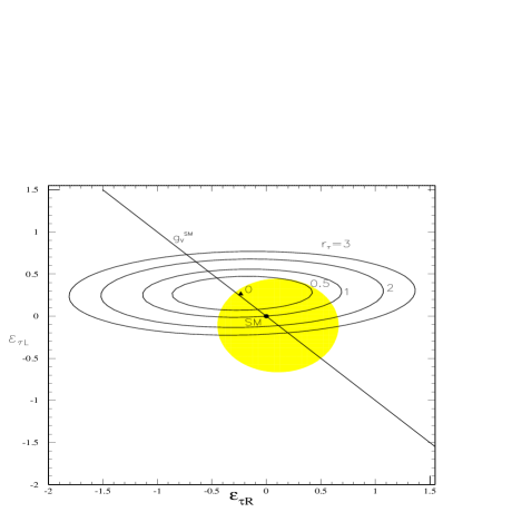
Figure 3: Left panel: experimental bounds on the NS interactions of $\nu_{e}$. The shaded area and the annulus (delimited by dotted lines) represent the parameter spaces for $\varepsilon_{eR},\varepsilon_{eL}$ allowed by data on $\nu_{e}e$ elastic scattering cross section and $e^{+}e^{-}\rightarrow\nu\bar{\nu}\gamma$ cross-section, respectively, at 99$\%$ C.L. [8]. Right panel: bounds on the NS interactions of $\nu_{\tau}$. The shaded area encloses the parameter space for $\varepsilon_{\tau R},\varepsilon_{\tau L}$ allowed by data the $e^{+}e^{-}\rightarrow\nu\bar{\nu}\gamma$ cross-section at $99\%$ C.L. [8]. On both panels, the contours for different values of $r_{e}$ and $r_{\tau}$ in the SK signal are also shown (solid curves). The SM case itself ($\varepsilon_{R,L}=0$) is indicated by filled circles, and $g^{SM}_{V}$ labels the lines along which $\varepsilon_{e(\tau)V}=0$.

The existing experimental limits on the parameters $\varepsilon_{eR,L}$ and $\varepsilon_{\tau R,L}$ are shown in Fig. 3. Here we also draw the solid line (denoted by $g_{V}^{\rm SM}$) along which $\varepsilon_{e(\tau)V}=0$, and thus the neutrino vector coupling to electrons is the same as in the SM. Therefore, along this direction of the parameter space long-baseline experiments would not be sensitive to such NS interactions since the neutrino potential in matter is the same as in the SM. For the same reason, $\varepsilon_{\tau V}=0$ implies no matter effects on the atmospheric $\nu_{\mu}\rightarrow\nu_{\tau}$ oscillation pattern.

Due to the SM multiplet structures, the NS interactions of neutrinos (3) in general emerge with other interactions involving their charged partners in the weak isodoublets [20] (for more details and a more model independent approach see [8]). As a matter of fact, the most severe laboratory bounds rather apply to the charged lepton NS interactions, and their strength can be at most several percents of $G_{F}$. However, as it was shown in ref. [8], these limits cannot be directly translated into limits for the NS couplings of neutrinos, for some conspiracy among the contributions of different operators cannot be excluded and neutrino NS couplings can be sizeable while charged-lepton NS interactions can be properly suppressed.

Now we discuss the role of the extra interactions (3) for the detection of solar neutrinos via their elastic scattering off electrons, which is relevant for Super-Kamiokande and Borexino experiments. For the sake of completeness, we consider the most general case when the solar $\nu_{e}$ oscillates into the active-sterile combination $\nu^{\prime}=s_{as}\nu_{a}+c_{as}\nu_{s}$ ($s_{as}=\sin\theta_{as},c_{as}=\cos\theta_{as}$), where the active component is $\nu_{a}=c_{23}\nu_{\mu}-s_{23}\nu_{\tau}$. The case $s_{as}=1$ corresponds to the $\nu_{e}\rightarrow\nu_{a}$ (fully active) conversion, whereas $s_{as}=0$ corresponds to the $\nu_{e}\rightarrow\nu_{s}$ (fully sterile) conversion. The expected energy spectrum of the recoil electrons is given by the following expression:

$$S(T)=\sum_{i}\phi_{i}\int dE\lambda_{i}(E)\left[{\displaystyle\frac{d\tilde{\sigma}_{\nu_{e}}}{dT}}P(E)+s_{as}^{2}\left(c^{2}_{23}{\displaystyle\frac{d\tilde{\sigma}_{\nu_{\mu}}}{dT}}+s^{2}_{23}{\displaystyle\frac{d\tilde{\sigma}_{\nu_{\tau}}}{dT}}\right)\left[1-P(E)\right]\right],$$ (5)

where $\phi_{i}$ are the fluxes of the solar neutrino sources which can be relevant for the signal ($i=^{8}$B, ⁷Be, $pp$ etc.), $\lambda_{i}(E)$ are the corresponding energy spectra (normalized to unity), and $P(E)$ is the generic survival probability of solar $\nu_{e}$ with the energy $E$. The differential cross sections are ($\alpha=e,\mu,\tau$):

$${\displaystyle\frac{d\tilde{\sigma}_{\nu_{\alpha}}(E,T)}{dT}}=\frac{2}{\pi}G^{2}_{F}m_{e}\int^{{T}^{\prime}_{\rm max}}_{0}dT^{\prime}~{}\rho(T,T^{\prime})\left[\tilde{g}^{2}_{\alpha L}+\tilde{g}^{2}_{\alpha R}\left(1-\frac{T^{\prime}}{E}\right)^{2}-\tilde{g}_{\alpha L}\tilde{g}_{\alpha R}\frac{m_{e}T^{\prime}}{E^{2}}\right],$$ (6)

where $T$ is the ‘reconstructed’ recoil electron kinetic energy, $T^{\prime}$ is the ‘true’ value given by the kinematics and ranging as $0\leq T^{\prime}\leq{T}^{\prime}_{\rm max}=\frac{E}{1+m_{e}/2E}$, and $\rho(T,T^{\prime})$ is the resolution function (explicitly given below). The possible non-standard interactions are included in the coupling constants $\tilde{g}_{\alpha L}$ and $\tilde{g}_{\alpha R}$ according to the re-definition shown in eq. (4). In the evaluation of $S(T)$ we also include the standard radiative corrections to the SM couplings (2) [21].

3 SNO versus Super-Kamiokande

The SNO and SK experiments are both dominated by the ⁸B neutrinos (neglecting the smaller flux of the hep neutrinos). The SNO experiments detects solar neutrinos with most significance via the CC reaction $\nu_{e}d\rightarrow ppe^{-}$ which is sensitive only to the $\nu_{e}$, while the SK is sensitive to all neutrino flavours through the $\nu_{\alpha}e\rightarrow\nu_{\alpha}e$ scattering, though the contribution of $\nu_{\mu,\tau}$ is about a factor 6 smaller than that of $\nu_{e}$. The measured fluxes normalized to the SSM prediction, $\phi_{B}^{\rm SSM}=5.05\times 10^{6}$ cm^-2s^-1 [22], are:

$$Z_{\rm SK}=0.459\pm 0.017,~{}~{}~{}~{}~{}~{}~{}Z_{\rm SNO}=0.347\pm 0.027,$$ (7)

from where we infer that the relative gap between the two signals may be filled by $\nu_{\mu,\tau}$-induced events in SK due to the solar neutrino conversion $\nu_{e}\rightarrow\nu_{a}$. This is the feature which disfavours the $\nu_{e}$ depletion exclusively into sterile neutrinos, in which case $Z_{\rm SK}=Z_{\rm SNO}$ would be expected.

To discuss the impact of the NS interactions we take the following point of view. First, in view of the absence of a significant spectral deformation as reported by both SK and SNO experiments, we assume that the $\nu_{e}$ survival probability $P$ does not depend on the energy, at least in the range explored by SK and SNO ($E_{e}>5$ MeV). Second, as the ⁸B flux is determined by the SSM with an accuracy of 20% or so, we treat it as a free parameter and parameterise it as $\phi_{B}=f_{B}\phi_{B}^{\rm SSM}$. Then the expected signals can be expressed as follows:

$$Z_{\rm SK}=f_{B}\left[r_{e}P+R^{\rm SM}_{\mu/e}s_{as}^{2}\left(c^{2}_{23}r_{\mu}+s^{2}_{23}r_{\tau}\right)(1-P)\right],~{}~{}~{}~{}~{}~{}Z_{\rm SNO}=f_{B}P,$$ (8)

where the ‘averaged’ cross section $R_{\alpha}$:

$$R_{\alpha}=\int{\mbox{d}}E\lambda_{B}(E)\tilde{\sigma}_{\nu_{\alpha}}(E),~{}~{}~{}~{}~{}~{}~{}\tilde{\sigma}_{\nu_{\alpha}}=\int^{T_{\rm max}}_{T_{\rm th}}dT~{}{\displaystyle\frac{d\tilde{\sigma}_{\nu_{\alpha}}(E,T)}{dT}}$$ (9)

are understood to include also the contributions from neutrino NS interactions, and the resolution function accounted in $\tilde{\sigma}_{\nu_{\alpha}}$ is

$$\rho(T,T^{\prime})={\displaystyle\frac{1}{\sqrt{2\pi}\sigma}}\exp\left[-\frac{(T-T^{\prime})^{2}}{2\sigma^{2}}\right],~{}~{}~{}~{}~{}~{}~{}~{}\sigma=\sigma_{0}\left(\frac{T^{\prime}}{\rm MeV}\right)^{1/2}.$$ (10)

For Super-Kamiokande $\sigma_{0}=0.47$ MeV, and the ‘reconstructed’ kinetic energy $T$ ranges between the threshold value $T_{\rm th}=(5~{}{\rm MeV}-m_{e})$ and ${T}_{\rm max}=(20~{}{\rm MeV}-m_{e})$. In eq. (8) the factors $r_{\alpha}=R_{\alpha}/R_{\alpha}^{\rm SM}$ ($\alpha=e,\mu,\tau$) parameterise the cross section deviation from the SM expectation $R^{\rm SM}_{\alpha}$ (i.e. from the limit $\varepsilon_{\alpha L,R}\rightarrow 0$), and $R_{\mu/e}^{\rm SM}=R^{\rm SM}_{\mu}/R^{\rm SM}_{e}$. In particular, for the electron energy threshold $E_{e}=5$ MeV it is $R^{\rm SM}_{\mu/e}\approx 0.158$.

For given values of the parameters $r_{e}$ and $r^{\prime}=s_{as}^{2}(c_{23}^{2}r_{\mu}+s_{23}^{2}r_{\tau})$, the combination of the SK and SNO signals determines both the $\nu_{e}$ survival probability and the Boron neutrino flux:

$$P^{-1}=1+\frac{1}{r^{\prime}R^{\rm SM}_{\mu/e}}\left(\frac{Z_{\rm SK}}{Z_{\rm SNO}}-r_{e}\right),~{}~{}~{}~{}~{}~{}f_{B}=P^{-1}Z_{\rm SNO}.$$ (11)

In particular, in the system of three standard neutrinos, with $s_{as}=1$ and $r_{e,\mu,\tau}=1$, we get $P=0.33\pm 0.10$ and $f_{B}=1.06\pm 0.42$, in agreement with the SSM prediction $f_{B}=0.84-1.2$.

Below we analyse both the case of $\nu_{e}$ conversion into the pure active state $\nu_{a}$ ($s_{as}=1$), and the case of $\nu_{e}$ conversion into the admixture of $\nu_{a}$ and $\nu_{s}$ ($s_{as}<1$). For simplicity, we assume that either $\nu_{e}$ or $\nu_{\tau}$ have NS interactions, though in general $\nu_{e}$ and $\nu_{\tau}$ may both have NS interactions.

3.1 Without sterile neutrino $(s_{as}=1)$

$\bullet$ Consider first the case when only $\nu_{e}$ has extra NS interactions: $\varepsilon_{eR,L}\neq 0$, $\varepsilon_{\tau R,L}=0$. Then the SK signal is insensitive to the flavour content of $\nu_{a}$ (i.e. to 23 mixing angle) and so we have $Z_{\rm SK}=f_{B}[r_{e}P+R^{\rm SM}_{\mu/e}(1-P)]$. Since the standard $\nu_{a}$ contribution to the SK signal is small, $R^{\rm SM}_{\mu/e}\approx 0.16$, we expect that too a big deviation from $r_{e}=1$, i.e. a $\nu_{e}$-induced contribution to the SK signal too far from the standard expectation, would cause an unacceptable mismatch between the SNO and SK signals. The results are shown in Fig. 1 (left panel). By comparing the $1\sigma$ allowed range of the SNO and SK signals, we see that within the SSM uncertainties for $f_{B}$ (delimited by dashed vertical lines), we obtain rather strong upper and lower bounds on $r_{e}$: $0.85\leq r_{e}\leq 1.25$. The allowed range for $r_{e}$ can be translated into allowed space for the parameters $\varepsilon_{eR,L}$. This is visualized in Fig. 3 (left panel). The parameter space allowed by the SK/SNO analysis is that delimited by the elliptical contours $r_{e}=0.85$ and $r_{e}=1.25$.

On the same Fig. 3 we also show the LSND limits obtained from the $\nu_{e}e$ elastic scattering (shaded area) and the LEP limits derived from $e^{+}e^{-}\rightarrow\nu\bar{\nu}\gamma$ process (area between dotted circles). We observe that the limits from the solar neutrino experiments are complementary to those from laboratory experiments, and in combination with the latter, provide very strong constraints on the extra interactions of $\nu_{e}$. Namely, there are two ‘disconnected’ allowed regions. The upper one, an horizontally elongated strip localized around the SM point ($\varepsilon_{eR},\varepsilon_{eL}$)=(0,0) delimited as:

$$-0.06\leq\varepsilon_{eL}\leq 0.15,~{}~{}~{}~{}~{}~{}~{}~{} ({\rm any}~{}\varepsilon_{eR}),$$ (12)

$$-0.5\leq\varepsilon_{eR}\leq 0.8,~{}~{}~{}~{}~{}~{}~{}~{} ({\rm any}~{}\varepsilon_{eL}).$$

The range for $\varepsilon_{eR}$ is in fact reduced to $-0.5\leq\varepsilon_{eR}\leq 0.6$ (for any $\varepsilon_{eL}$) if also the reactor $\bar{\nu}_{e}$ bounds are considered [8]. In the following we shall most focus on the SM neighborhood $(\varepsilon_{eR},\varepsilon_{eL})=(0,0)$ and so consider as allowed region that parameterised by $\varepsilon_{eL}=0,|\varepsilon_{eR}|\leq 0.5$. The lower region is the smaller strip elongated along the direction $\varepsilon_{eL}\sim-1.4$, with minor statistical significance. In addition, it is not appropriate for the MSW solution since strongly diminishes (or even makes negative) the matter potential of $\nu_{e}$. Therefore, in the following analysis we disregard this parameter region.

$\bullet$ The same procedure can be applied when only $\nu_{\tau}$ has NS interactions: $\varepsilon_{\tau R,L}\neq 0$, $\varepsilon_{eR,L}=0$. In this case we have $Z_{\rm SK}=f_{B}[P+r^{\prime}R^{\rm SM}_{\mu/e}(1-P)]$, where the $\nu_{\tau}$ contribution depends on the 2-3 mixing angle of neutrinos, $r^{\prime}=c_{23}^{2}+s_{23}^{2}r_{\tau}$. For the sake of definiteness, we consider the case of maximal 2-3 mixing, as motivated by the atmospheric neutrino observations, which results in $\nu_{a}=(\nu_{\mu}-\nu_{\tau})/\sqrt{2}$, and thus $r^{\prime}=\frac{1}{2}(1+r_{\tau})$. The results are shown in Fig. 1 (right panel). We observe that for large enough Boron flux, $f_{B}\raise 1.29167pt\hbox{$\;>$\kern-7.5pt\raise-4.73611pt\hbox{$\sim\;$}}1.2$, $r_{\tau}$ could go to zero as the SK signal would be recovered by the standard contribution of $\nu_{\mu}$. Therefore, in this case $\nu_{\tau}$ is allowed to behave like a ‘sterile’ state ($r_{\tau}=0$ means that the standard couplings to electrons are exactly canceled by the NS couplings, $\varepsilon_{\tau R,L}=-g_{R,L}$). On the contrary, for $f_{B}<1.3$ the $\nu_{\tau}$ cross section could be larger than the SM one. We observe that within the SK/SNO signal and the SSM uncertainties, $r_{\tau}$ could vary in the range from 0 to about 3. Correspondingly, the allowed range of $r^{\prime}$ is $0.5\raise 1.29167pt\hbox{$\;<$\kern-7.5pt\raise-4.73611pt\hbox{$\sim\;$}}r^{\prime}\raise 1.29167pt\hbox{$\;<$\kern-7.5pt\raise-4.73611pt\hbox{$\sim\;$}}2$.

The contours of $r_{\tau}$ as a function of $\varepsilon_{\tau R,L}$, are shown in Fig. 3 (left panel). The comparison with the LEP limits shown on the same Fig. 3 (shaded region) demonstrates that the $1\sigma$-limit $r_{\tau}\raise 1.29167pt\hbox{$\;<$\kern-7.5pt\raise-4.73611pt\hbox{$\sim\;$}}3$ inferred from the SK/SNO signal analysis, considerably restricts the allowed parameter space of $\varepsilon_{\tau R,L}$. Most conservatively, ignoring any correlation, the allowed range for individual parameters is

$$-0.23\leq\varepsilon_{\tau L}\leq 0.45~{}~{}~{}~{}~{} ({\rm any}~{}\varepsilon_{\tau R}),$$ (13)

$$-0.45\leq\varepsilon_{\tau R}\leq 0.65,~{}~{}~{}~{}~{} ({\rm any}~{}\varepsilon_{\tau L}).$$

In conclusion, even if the bounds on $\nu_{\tau}$ NS interactions obtained by solar neutrino experiments are comprehensively much weaker than the LEP bounds, they are complementary and, in particular, cut out the parameter space corresponding to large negative values of $\varepsilon_{\tau L}$.

3.2 The active-sterile conversion $(s_{as}<1)$

$\bullet$ Let us first analyse the conversion $\nu_{e}\rightarrow\nu^{\prime}=s_{as}\nu_{a}+c_{as}\nu_{s}$, where $\nu_{e}$ and $\nu_{\tau}$ are assumed to have only SM interactions. Hence in eq. (8) the SK signal gets simplified into $Z_{\rm SK}=f_{B}[P+s_{as}^{2}(1-P)R^{\rm SM}_{\mu/e}]$. So upon comparing the SNO and SK signals, for a given $f_{B}$ we can constrain the magnitude of the active fraction, $s_{as}^{2}$. In Fig. 2 we show the allowed 1$\sigma$ region in the plane ($f_{B},s^{2}_{as}$) (left panel). As we could expect, $s_{as}^{2}$ cannot vanish even in the asymptotic regime of very large $f_{B}$, and so the pure sterile conversion is strongly disfavoured. For the ‘central value’ of the Boron flux ($f_{B}=1$) we find $s^{2}_{as}\geq 0.7$, while for $f_{B}=1.2$ also $s^{2}_{as}=0.5$ can be allowed which would correspond to maximal $\nu_{a}-\nu_{s}$ mixing. As for the $\nu_{e}$ survival probability, $P=Z_{\rm SNO}/f_{B}$, the SSM range $f_{B}=0.84-1.2$ implies that $0.32\raise 1.29167pt\hbox{$\;<$\kern-7.5pt\raise-4.73611pt\hbox{$\sim\;$}}P\raise 1.29167pt\hbox{$\;<$\kern-7.5pt\raise-4.73611pt\hbox{$\sim\;$}}0.38$ (at 1-$\sigma$).

$\bullet$ Let us now assume that $\nu_{e}$ have some NS couplings with the electron, i.e. $\varepsilon_{eR,L}\neq 0$. Now we have to refer to the more general expression for $Z_{\rm SK}$ displayed in eq. (8), with $r^{\prime}=s_{as}^{2}$. Then for given $f_{B}$, we have $P=Z_{\rm SNO}/f_{B}$, and so the first equation in eq. (11)) describes the correlation between $r_{e}$ and $r^{\prime}=s_{as}^{2}$. The corresponding isocontours are presented in Fig. 2 (right panel). Now we observe that by increasing the $\nu_{e}$ cross section, in the range $r_{e}\sim 1.2-1.5$, the completely sterile conversion ($s_{as}=0$) can be also allowed. Notice that for $s^{2}_{as}\rightarrow 0$ all curves in Fig. 2, corresponding to different values of $f_{B}$, are attracted to the ‘fixed’ points, $r_{e}=1.2,1.5$. The reason is that for $r^{\prime}=0$, the two eqs. (8) degrade to $Z_{\rm SNO}=f_{B}P$ and $Z_{\rm SK}=f_{B}Pr_{e}$, which can be satisfied, independently of $f_{B}$, if and only if $r_{e}=Z_{\rm SK}/Z_{\rm SNO}$. For the central values of $Z_{\rm SK}$ and $Z_{\rm SNO}$ this would correspond to $r_{e}=1.32$, while within $1\sigma$ uncertainty in (7), we can have $r_{e}=1.2-1.5$. As we see from the Fig. 3, this possibility is still allowed by the LSND data on $\nu_{e}e$ scattering and the collider data on $e^{+}e^{-}\rightarrow\nu_{e}\bar{\nu}_{e}\gamma$ cross section.

The same exercise has been repeated by allowing $\nu_{\tau}$ to have the NS interactions. However, in this case we do not get more information than what we obtained in Sec. 3.1. The admixture with the sterile neutrino simply re-scales the allowed range for the parameter $r^{\prime}=(1+r_{\tau})/2$, viz. $0.5\raise 1.29167pt\hbox{$\;<$\kern-7.5pt\raise-4.73611pt\hbox{$\sim\;$}}r^{\prime}\raise 1.29167pt\hbox{$\;<$\kern-7.5pt\raise-4.73611pt\hbox{$\sim\;$}}2$, just by the factor $s_{as}^{-2}$.

3.3 Spectral deformation at Super-Kamiokande

We have seen that the solar neutrino experiments contribute further in constraining the parameter $\varepsilon_{eL}$, with respect to the LSND experiment. For example, for $\varepsilon_{eR}=0$, the values $r_{e}=0.85,1,1.25,1.5$ correspond to $\varepsilon_{eL}=-0.05,0,0.07,0.16$, respectively, to be compared with the LSND limits $-0.04<\varepsilon^{e}_{L}<0.08$ ($68\%$ C.L.) and $-0.15<\varepsilon^{e}_{L}<0.17$ ($99\%$ C.L.). On the other hand, the SK/SNO analysis provides much looser limits on $\varepsilon_{eR}$. Therefore, as already discussed, we consider the range $|\varepsilon_{eR}|\leq 0.5$ obtained by comparing the LSND and LEP data with the data from $\bar{\nu}_{e}e$ scattering at reactors [8]. The different sensitivity of the solar neutrino experiments to $\varepsilon_{eL}$ and $\varepsilon_{eR}$ (or analogously to $\varepsilon_{\tau L}$ and $\varepsilon_{\tau R}$) is easy to understand. The magnitude of the total signal in SK, as well as of the cross section measured at LSND, is mostly controlled by the $\tilde{g}^{2}_{eL}$-term in the cross section. As a matter of fact both the LSND data and the SK/SNO analysis imply, around the point $(\varepsilon_{eR},\varepsilon_{eL})=(0,0)$, that $\tilde{g}_{eL}$ should not deviate too much from the SM prediction $g_{L}=\sin^{2}\theta_{W}+1/2$. On the other hand, as one can see from eq. (6), the parameter $\tilde{g}_{eR}$ controls the energy dependence of the recoil electron spectrum. Therefore, at this point, we may wonder about the implications of NS interactions with electrons for the energy spectrum measured at SK (since in the above we have considered only the global rates). Without entering into a detailed $\chi^{2}$ analysis, which is beyond our scope, we have performed a scanning of the $\varepsilon_{eR},\varepsilon_{eL}$ and $P$ space, and we have realized that $\varepsilon_{eR}$ is poorly constrained. For the sake of demonstration, in Fig. 4 (left panel) we show the spectral deformation expected at SK for several values of $\varepsilon_{eR}$ in the interval $-0.4\div 0.4$, taking $\varepsilon_{eL}=0$. We can observe quite small deviations from the SM case. On the right panel of the same Fig. 4 we show the spectral deformations for different values of $\varepsilon_{\tau R}$ within the experimentally allowed interval. The reason of this poor sensitivity of the SK recoil electron spectrum to $\varepsilon_{e(\tau)R}$ is that it is smoothed out by the integration over the continuous Boron neutrino spectrum. We will see in next section that the mono-energetic character of the Beryllium neutrinos makes the Borexino detector more sensitive to these NS couplings.

4 Predictions for Borexino

We consider as prototype for our discussion the Borexino experiment which is aimed to detect mono-energetic ⁷Be neutrinos via $\nu e$ elastic scattering [23]. Eq. (5) shows the advantage of using mono-energetic neutrinos, with $\lambda(E)=\delta(E-E_{0})$ and $E_{0}$ is the neutrino line energy. In this case the smearing of the electron energy distribution due to the integration over the neutrino spectrum is absent. Therefore, while the expected global rate substantially depends on the $\nu_{e}$ survival probability $P=P(E_{0})$, the shape of the recoil electron spectrum does not get substantially deformed in the SM scenario ($\varepsilon_{\alpha L,R}=0$). Thus, for mono-energetic neutrinos a distortion of the electron energy distribution would be an unambiguous evidence of neutrino non-standard interactions. This would represent a unique signature of new physics that may be provided by solar neutrino experiments.

The Beryllium neutrino flux, with $E_{0}=0.862$ MeV, can be measured by exploring the energy window $T=0.25-0.66$ MeV for the recoil electron: 0.25 is the attainable detection threshold and 0.66 is the Compton edge. In this window, 80% of the signal is from the ⁷Be neutrinos, while the rest comes from the CNO and $pep$ neutrinos. In fact, both the edges get smeared when the energy resolution is taken into account and the lower part of the spectrum is arisen by the $pp$ and ⁷Be$(0.38{\rm MeV})$ neutrinos. These features are clearly apparent in Fig. 5 (upper left panel) where the energy distributions of the expected events are plotted. The resolution function used is of the form given in eq. (10) with width $\sigma_{0}=57.7$ KeV [24]. We see that in the interval $T=0.3-0.6$ MeV the spectral shape is quite regular with almost constant slope.

Now let us turn to neutrino oscillations. The several scenarios proposed to explain the SNA predict different survival probabilities for the beryllium neutrinos. For example the suppression can be quite strong, $P\raise 1.29167pt\hbox{$\;<$\kern-7.5pt\raise-4.73611pt\hbox{$\sim\;$}}0.2$ in case of small-mixing angle MSW conversion, but can be weaker, $P\sim 0.3-0.7$ in case of vacuum oscillation or large-mixing angle MSW conversion. On the other hand, as mentioned, neutrino conversions are expected not to distort the energy distribution as long as $\nu_{\mu,\tau}$ have only SM interactions. Then the energy spectrum will be just re-scaled with a slope which will be in between that of the SSM distribution and that expected in case of complete depletion of solar $\nu_{e}$. The energy distributions shown in the upper right panel of Fig. 5 for different values of $P$, assuming that all neutrinos have the standard model couplings, can help to figure out the standard situation. Notice that when all $\nu_{e}$’s are converted into $\nu_{a}$ ($P=0$) the distribution becomes flatter in the range $T=(0.3-0.6)$ MeV (lowest curve).

We now discuss how this picture gets modified when NS interactions of neutrinos are switched on. In the following, in view of the results obtained in the previous section, the parameters $\varepsilon_{e,\tau L}$ are set to zero, whereas the parameters $\varepsilon_{e,\tau R}$ are varied into the corresponding allowed ranges. The lower plots in Fig. 5 represent the expected event distribution at Borexino as a result of $\nu_{e}\rightarrow(\nu_{\mu}-\nu_{\tau})/\sqrt{2}$ transition for different values of $P$ and for $\varepsilon_{eR}=0.4,-0.3$ and $\varepsilon_{\tau R}=0.6,-0.3$. By comparing the analogous SM cases (upper plots), we observe for positive $\varepsilon_{e,\tau R}$ a strong deformation of the energy distribution, with a noticeable negative slope accompanied by an increase of the number of events. We also see that the case in which only $\varepsilon_{eR}$ is switched on can be distinguished by the one in which only $\varepsilon_{\tau R}$ is on. In the former case the decreasing of the spectrum is even sharper. The presence of the background in the lower-energy end may render hard to observe the part mostly deformed. However, due to the exponential decay of the background it is still possible to reveal the deformation above (0.4 - 0.45) MeV. On the other hand, for negative $\varepsilon_{e,\tau R}$ the previous strong spectral deformation is lost, but the spectrum becomes flatter as $P$ becomes smaller.

We have then made more apparent the comparison between the SM picture and that in which neutrinos have also NS interactions. We have compared the electron energy spectra obtained for different $\varepsilon_{e,\tau R}$ but normalized to the same number of total events $N_{\rm tot}$ in the energy window $T=0.3-0.6$ MeV (where essentially only ⁷Be neutrinos contribute). For definiteness, we have $N_{\rm tot}=23$ corresponding to $P=0.5$ and $\varepsilon_{e,\tau R}=0$. Then for each value of $\varepsilon_{e,\tau R}$ the corresponding $\nu_{e}$ or $\nu_{\tau}$ cross section is evaluated, i.e the parameter $r_{e,\tau}$, while $P$ is determined by imposing $N_{\rm tot}=23$. The energy spectra (divided by the SSM prediction, i.e. taking $P=1$, $\varepsilon_{e,\tau R}=0$) are displayed in Fig. 6 (upper panels). For example, for $\varepsilon_{eR}>0$ (left panel) the spectrum is very deformed with a negative slope. On the other hand, for $\varepsilon_{eR}\sim-0.3$ the slope becomes positive, though the deformation is less pronounced.

Notice that in the case of the SK spectra, analysed in Fig. 4 the slope never becomes positive, even for negative values of either $\varepsilon_{eR}$ or $\varepsilon_{\tau R}$. This different behaviour can be qualitatively understood by considering the derivative of the $\nu e$ differential cross section:

$$\frac{{d}}{{d}T}\left[\frac{d\sigma_{\nu_{\alpha}}(E,T)}{dT}\right]\propto-2\left(1-\frac{T}{E}\right)-\frac{\tilde{g}_{\alpha L}}{\tilde{g}_{\alpha R}}\frac{m_{e}}{E}.$$ (14)

This is understood to be convoluted with the neutrino spectrum $\lambda(E)$. Then the slope becomes less negative as the second term dominates over the first, i.e. for $E\sim T$ and ${\tilde{g}_{\alpha L}}/{\tilde{g}_{\alpha R}}<0$, and at the same time the width of the neutrino spectrum is narrow enough to resolve this term, that is $\lambda(E)\raise 1.29167pt\hbox{$\;<$\kern-7.5pt\raise-4.73611pt\hbox{$\sim\;$}}|\frac{\tilde{g}_{\alpha L}}{\tilde{g}_{\alpha R}}|\frac{m_{e}}{2E}$. Notice that in the SM case, ${{g}_{L}}/{{g}_{R}}>0$ for $\nu_{e}$ and ${{g}_{L}}/{{g}_{R}}<0$ for $\nu_{\tau}$. Then the derivative (14) cannot become positive for the continuous ⁸B spectrum. On the other hand, for the mono-energetic ⁷Be neutrinos it can even for $\varepsilon_{\alpha R,L}=0$ when, for example, $P$ is small enough so that the contribution to the signal of $\nu_{a}$ gets increased and the role of the interference term in the differential cross section gets enhanced. Clearly, by switching on the NS couplings this effect can be further emphasized as the spectra displayed in Fig. 6 show. The spectral deformation can be experimentally probed by sub-dividing the energy window considered so far into the two symmetric windows which visually emerge from these plots, $\Delta T_{1}=3-4.5$ MeV and $\Delta T_{2}=4.5-6$ MeV, and comparing the respective number of events $N_{1}$ and $N_{2}$. For this purpose, we have introduced the asymmetry parameter $\delta$:

$$\delta={\displaystyle\frac{N_{1}-N_{2}}{N_{1}+N_{2}}}.$$ (15)

From the upper plots of Fig. 6, we can see that the asymmetry $\delta$ is 0.046 for $\varepsilon_{R}=0$ and further diminishes for negative values of $\varepsilon_{eR}$, while it increases for positive $\varepsilon_{eR}$, up to 11% for $\varepsilon_{eR}=0.4$. The same behaviour occurs when $\varepsilon_{\tau R}$ are non-vanishing, though both the increasing and the decreasing is less dramatic. Finally, the lower panel of Fig. 6 shows the correlation between the total signal $N_{\rm tot}=N_{1}+N_{2}$ and the event difference $N_{1}-N_{2}$ (i.e. the asymmetry $\delta$) for different values of $\varepsilon_{eR}$ (solid lines) and $\varepsilon_{\tau R}$ (dashed lines) and for comparison with the SM case (dotted line). These curves demonstrate that the joint measurement of $N_{\rm tot}$ and $N_{1}-N_{2}$ could reveal the presence of neutrino NS interactions. In the SM case, the asymmetry is almost independent of $N_{\rm tot}$ in the interval $N_{\rm tot}=17-38$, (corresponding to the survival probability in the range $P=0.3-1$) as it varies from $\delta\simeq 0.044$ to $\delta\simeq 0.046$, and it approaches the minimal value $\delta\simeq 0.037$ for $N_{\rm tot}=8.3$ ($P=0$), when the signal is only contributed by the $\nu_{\mu,\tau}e$ scattering. For non-vanishing $\varepsilon_{eR}$, the variation of the parameter $\delta$ with respect to $N_{\rm tot}$ is more pronounced. Namely, in the interval $N_{\rm tot}=17-38$ (corresponding incidentally to the same interval $P=0.3-1$) the asymmetry varies from $0.10$ to 0.13 and for smaller $N_{\rm tot}$ it sharply decreases. This asymmetry parameter or, equivalently, the measurement of the difference $N_{1}-N_{2}$ should be statistically significant for one-year of data taking. For example, by taking $P=0.5$, we expect in the SM case $N_{\rm tot}\simeq 8400$ per year and a difference of events $N_{1}-N_{2}\simeq 380$ which is larger than the statistical fluctuation. Analogously for $\varepsilon_{eR}=0.4$, we find the same $N_{\rm tot}$ per year, but an even more statistically significant difference of events, $N_{1}-N_{2}\simeq 940$. The cases with non-vanishing $\varepsilon_{\tau R}$ show a less dramatic effect with respect to the SM case, unless $\varepsilon_{\tau R}\raise 1.29167pt\hbox{$\;>$\kern-7.5pt\raise-4.73611pt\hbox{$\sim\;$}}0.2$. Notice, that it may be essential to make use of the interplay between the measurement of the the energy spectrum $S(T)$ and the corresponding asymmetry $\delta$ to better disentangle scenarios with different NS couplings (either $\varepsilon_{eR}$ or $\varepsilon_{\tau R}$ or both non zero).

5 Conclusions

Extensions of the Standard Model generally include new neutral current interactions that can be flavour changing as well as flavour conserving. In this respect, the recent NuTeV data are very encouraging and should be further considered.

In this paper, we have re-examined the implications for solar neutrino detection of non-standard flavour conserving interactions of neutrinos with the electron. In particular, we have payed special attention to the case in which $\nu_{\tau}$ and $\nu_{e}$ have non-standard couplings with the electron. In the light of the atmospheric neutrino data pointing to a large mixing between $\nu_{\mu}$ and $\nu_{\tau}$, the solar neutrino deficit can now be regarded as the ‘conversion’ of $\sim$ 65% of solar $\nu_{e}$’s into an equal amount of $\nu_{\mu}$ and $\nu_{\tau}$. We have found that present solar neutrino experiments show a complementary sensitivity in the parameter space with respect to that achieved by laboratory neutrino experiments. We have so tried to reverse the point of view by looking for some signature of such NS interactions within the allowed parameter space. We have demonstrated that the allowed range for these neutrino non-standard interactions could be tested by Borexino experiment, aimed to detect the monochromatic ⁷Be-line. Indeed, neutrino NS interactions could manifest especially through an unexpected spectral deformation and in some cases with an ‘anomalous’ increase of the number of total events. Therefore, the Borexino experiment can be a unique tool to test solar neutrinos as well as the Standard Model itself. Now we would like to comment on an issue related to future low-energy neutrino experiments. For the sake of simplicity, we consider only ⁷Be neutrinos. Then we consider the following function, normalized to the SSM expectation:

$$F(T)={\displaystyle\frac{c^{2}_{23}{\displaystyle\frac{d\tilde{\sigma}_{\nu_{\mu}}(E,T)}{dT}}+s^{2}_{23}{\displaystyle\frac{d\tilde{\sigma}_{\nu_{\tau}}(E,T)}{dT}}}{{\displaystyle\frac{d\tilde{\sigma}_{\nu_{e}}(E,T)}{dT}}}}.$$ (16)

This observable $F(T)$ can be in fact built up by subtracting from the energy distribution $S(T)$ measured at Borexino the survived $\nu_{e}$ contribution as ‘directly’ measured by a low-energy neutrino experiment such as LENS – sensitive only to the $\nu_{e}$ flavour [26]. In this way we would more directly test the $\nu_{\mu},\nu_{\tau}$ contribution to the energy distribution and so test $\nu_{\tau}$ NS interactions. This complementary role between these two kinds of experiments is analogous to that presently played by SK and SNO for the high-energy ⁸B neutrinos.

Finally, we would like to comment about the possibility, which is usually neglected, to solve the solar neutrino deficit with matter oscillations induced by flavour-changing and flavour-conserving NS interactions of neutrinos with electrons (with massless neutrinos) [12]. Indeed, also such flavour-changing NS interactions (the relevant flavour-changing parameters would be $\varepsilon_{e\beta V},~{}\beta=\mu,\tau$) are not strongly constrained [8] and, jointly with the flavour-diagonal NS ones, can give rise to a sizeable mixing angle in matter. Therefore, it could be worth re-considering such conversion mechanism.

Acknowledgments We thank L. Girlanda and P. Ronchese for ‘graphics’ assistance. The work of Z. B. was in part supported by the MURST Research Grant ”Astroparticle Physics” and that of A. R. by the European Union under the contracts HPRN-CT-2000-00148 (Across the Energy Frontier).

Figure 1: Analysis of the SK and SNO data for the conversion $\nu_{e}\rightarrow\nu_{a}=c_{23}\nu_{\mu}-s_{23}\nu_{\tau}$. In the left panel only $\nu_{e}$ is considered to have the NS couplings with electrons ($r=r_{e}$), while in the right panel only $\nu_{\tau}$ ($r=r_{\tau}$), and maximal mixing is assumed, $\theta_{23}=45^{\circ}$. The contours of the 1$\sigma$ allowed region are shown by solid curves (the dotted lines in the middle refers to the central values of SK and SNO data). The range of $f_{B}$ allowed by the SSM uncertainties is delimited by vertical dashed lines ($f_{B}=1$ corresponds to the reference SSM model). As a guideline for the reader we have drawn (black squares) some points for the $\nu_{e}$ survival probability which for given $f_{B}$ is fixed by the SNO signal, $P=Z_{\rm SNO}/f_{B}$.

Figure 2: Analysis of SK and SNO data regarding the conversion $\nu_{e}\rightarrow\nu^{\prime}=s_{as}\nu_{a}+c_{as}\nu_{s}$ ($\nu_{s}$ is a sterile neutrino). On the left panel the standard case ($\varepsilon_{R,L}=0$) is illustrated in the plane scanned by the paramemers $f_{B}$ and $s^{2}=s^{2}_{as}$; the solid contours delimit the region allowed by the SK/SNO signals (8) at 1$\sigma$, the dotted curve in the middle corresponds to the central values of $Z_{\rm SK}$ and $Z_{\rm SNO}$. The values of $P$ are indicated by black squares. On the right panel the effect of NS interactions of $\nu_{e}$ is accounted in the plane ($r_{e},s^{2}$). The ‘oblique’ solid lines delimit the parameter space allowed by SK/SNO for $f_{B}=1$, while the effect of varying $f_{B}$ within $0.84-1.2$ is accounted by dot- and dash-lines respectively. The corresponding survival probabilities $P=Z_{\rm SNO}/f_{B}$ are also indicated along these lines.

Figure 4: Left panel: SK energy spectra (divided by the SSM expectation) versus the recoil electron energy $E_{e}$ for different values of $\varepsilon_{eR}$ in the allowed range ($\varepsilon_{eR}=0.4,0.2,-0.2,-0.4$), and $\varepsilon_{eL}=0$. The SK experimental data (with the corresponding error) are also shown [2]. Right panel: the same but for different values of $\varepsilon_{\tau R}$ ($\varepsilon_{\tau L}=0$). All spectra are normalized to the central value of $Z_{SK}$ through the constraints (see eq. (11)) imposed on $P$ and $f_{B}$ by the experimental central values of $Z_{SK}$ and $Z_{SNO}$ for given $\varepsilon_{eR}(\varepsilon_{\tau R})$ i.e. $r_{e}(r_{\tau})$ (as indicated). The inferred values of $P,f_{B}$ are also shown.

Figure 5: Upper left panel: the event distribution in Borexino experiment versus the recoil electron kinetic energy $T$, as expected for the SSM predicted fluxes ($P=1$) and with no extra interactions ($\varepsilon_{L,R}=0$). The dotted curve shows the signal due to only ⁷Be neutrinos ($E=0.38,0.86$ MeV), while the dashed curve indicates the contribution from all other relevant solar $\nu_{e}$ sources ($pp$, $pep$, CNO etc.). The total expected signal is shown by the solid curve. Upper right panel: the effect on the energy distribution of the events due to the neutrino conversion $\nu_{e}\rightarrow\nu_{a}$ for different survival probabilities $P$. Lower panels show how the event distribution gets modified for non-zero $\varepsilon_{eR}$ (left) or $\varepsilon_{\tau R}$ (right) for different suervival probabilities ($\varepsilon_{e,\tau L}=0$ is understood everywhere).

Figure 6: Upper panels: $S(T)/S_{0}(T)$ is the ratio of the electron energy spectrum for non-vanishing $\varepsilon_{eR}$ (left panel) and $\varepsilon_{\tau R}$ (right panel) with that expected from the SSM (and $\varepsilon_{e,\tau R}=0)$ at Borexino. All curves are normalized in such a way that the total number of events be $N_{\rm tot}=23$ per day in the interval $T=0.3-0.6$ MeV (obtained with $P=0.5$ in the SM case, $\varepsilon_{R}=0$). The corresponding values of $r_{e}$ (or $r_{\tau}$), $P$ and the asymmetry $\delta$ are also indicated. Lower panel: The correlation between the expected $N_{\rm tot}$ and the difference of events $N_{1}-N_{2}$ in the energy windows $\Delta T_{1}=(0.3-0.45)$ MeV, $\Delta T_{2}=(0.45-0.6)$ MeV, for several values of NS couplings $\varepsilon_{eR}$ (solid lines) and $\varepsilon_{\tau R}$ (dashed lines). The SM case ($\varepsilon_{e,\tau R}=0$) is depicted by dotted line. For $\varepsilon_{eR}\neq 0$, the variation of $N_{\rm tot}$ from $\simeq 8.3$ to $\simeq 38-44$ is due to the corresponding change of the survival probability $P$ from 0 to 1. For $\varepsilon_{\tau R}\neq 0$ and $P=0$, $N_{\rm tot}$ varies according to $\varepsilon_{\tau R}$ – e.g. $N_{\rm tot}\simeq 13$ or 10 for $\varepsilon_{\tau R}=0.6$ or 0.2, respectively. In this case, all curves clearly converge to $N_{\rm tot}\simeq 38$ for $P=1$.

References

- [1] T. Toshito [SuperKamiokande Collaboration], arXiv:hep-ex/0105023.
- [2] S. Fukuda et al. [Super-Kamiokande Collaboration], Phys. Rev. lett. 86 (2001) 5651.
- [3] Q. Ahmad et al. [SNO Collaboration], Phys. Rev. lett. 87 (2001) 071301.
-
[4]
For a recent review, see for example:
M. C. Gonzalez-Garcia, M. Maltoni, C. Pena-Garay and J. W. F. Valle,
Phys. Rev. D 63 (2001) 033005;
G. L. Fogli, E. Lisi, A. Marrone, D. Montanino and A. Palazzo, hep-ph/0104221. -
[5]
V. Barger, D. Marfatia and K. Whisnant,
hep-ph/0106207;
J. N. Bahcall, M. C. Gonzalez-Garcia and C. Pena-Garay, hep-ph/0106258;
P. I. Krastev and A. Y. Smirnov, hep-ph/0108177 - [6] M. Apollonio et al. [CHOOZ Collaboration], Phys. Lett. B 466 (1999) 415.
- [7] G. P. Zeller et al. [NuTeV Collaboration], hep-ex/0110059.
- [8] Z. Berezhiani and A. Rossi, hep-ph/0111137.
- [9] Z. Berezhiani and A. Rossi, Phys. Rev. D 51 (1995) 5229.
-
[10]
S. P. Mikheev and A. Yu. Smirnov, Nuovo Cim. C 9 (1986) 17;
L. Wolfenstein, Phys. Rev. D 17 (1978) 2369. -
[11]
L. Wolfenstein, ref. [11];
J. W. F. Valle, Phys. Lett. B 199 (1987) 432;
E. Roulet, Phys. Rev. D 44 (1991) 935;
M. M. Guzzo, A. Masiero and S. T. Petcov, Phys. Lett. B 260 (1991) 154. - [12] V. Barger, R. J. Phillips and K. Whisnant, Phys. Rev. D 44 (1991) 1629.
- [13] Z. G. Berezhiani and A. Rossi, Proc. of the 5th Int. Workshop on ‘Neutrino Telescopes’, p. 123-135, ed. by M. Baldo Ceolin, Venice, Italy, 1993; hep-ph/9306278; Nucl. Phys. Proc. Suppl. 35 (1994) 469.
- [14] S. Bergmann, M. M. Guzzo, P. C. de Holanda, P. I. Krastev and H. Nunokawa, Phys. Rev. D 62 (2000) 073001 and references therein.
- [15] C. McGrew [Super-Kamiokande Collaboration], Proc. of the 9th Int. Workshop on ‘Neutrino Telescopes’, vol.1, p.93, ed. by M. Baldo Ceolin, Venice, Italy, 2001.
- [16] M. Nakamura [DONUT Collaboration], Nucl. Phys. Proc. Suppl. 77 (1999) 259. B. Lundberg [DONUT Collaboration], Nucl. Phys. Proc. Suppl. 91 (2001) 233.
- [17] P. Vilain et al. [CHARM-II Collaboration], Phys. Lett. B 335 (1994) 246.
- [18] N. Fornengo et al., hep-ph/0108043.
- [19] G. L. Fogli, E. Lisi and A. Marrone, Phys. Rev. D 63 (2001) 053008; hep-ph/0105139.
-
[20]
S. Bergmann, Y. Grossman and D. M. Pierce,
Phys. Rev. D 61 (2000) 053005;
S. Bergmann et al. Phys. Rev. D 62 (2000) 073001. - [21] J. N. Bahcall, M. Kamionkowski and A. Sirlin, Phys. Rev. D 51 (1995) 6146.
- [22] J. Bahcall, M. Pinsonneault and S. Basu, astro-ph/0010346.
-
[23]
C. Arpesella et al. [BOREXINO Collaboration], Proposal of Borexino, 1991
(unpublished);
G. Ranucci et al. [BOREXINO Collaboration], Nucl. Phys. Proc. Suppl. 91 (2001) 58. - [24] G. Bellini [BOREXINO Collaboration], Nucl. Phys. Proc. Suppl. 48 (1996) 363.
- [25] E. Meroni [BOREXINO Collaboration], Nucl. Phys. Proc. Suppl. 100 (2001) 42; G. Alimonti et al. [BOREXINO Collaboration], Astropart. Phys. 16 (2002) 205.
- [26] R. S. Raghavan, Phys. Rev. Lett. 78, 3618 (1997).
- [27] M. M. Guzzo, H. Nunokawa, P. C. de Holanda and O. L. Peres, Phys. Rev. D 64 (2001) 097301.