SINP/TNP/01-25

Accepted in Physics Letters B

Viability of bimaximal solution of the Zee mass matrix

Biswajoy Brahmachari and Sandhya Choubey

Theoretical Physics Group

Saha Institute of Nuclear Physics

1/AF Bidhannagar, Kolkata-700064, India

We know $L_{e}-L_{\mu}-L_{\tau}$ symmetry gives $m^{2}_{1}=m^{2}_{2}>>m^{2}_{3}$ pattern in Zee model. $\Delta m^{2}_{\odot}$ emerges from a small breaking of this symmetry. Because this symmetry is broken very weakly $\theta_{\odot}$ does not deviate much from $\tan^{2}\theta_{\odot}=1$ which is its value in the symmetric limit. This gives a mismatch with LMA solution where mixing is large but not exactly maximal. We confront this property of Zee mass matrix by phenomenologically analyzing recent results from solar and atmospheric neutrino oscillation experiments at various confidence levels. We conclude that LOW type solution is compatible with the Zee mass matrix at 99% confidence level when atmospheric neutrino deficit is explained by maximal $\nu_{\mu}\leftrightarrow\nu_{\tau}$ oscillation. Thus the minimal version of the Zee model even though disfavored by the LMA type or VO type solutions, is compatible with LOW type solution of solar neutrino problem.

The neutrino mass matrix under the Zee ansatz [1] can be written in the flavor basis as

$${\cal M} = {\pmatrix{0&\mbox{$m_{e\mu}$~{}}&\mbox{$m_{e\tau}$~{}}\cr\mbox{$m_{e\mu}$~{}}&0&\mbox{$m_{\mu\tau}$~{}}\cr\mbox{$m_{e\tau}$~{}}&\mbox{$m_{\mu\tau}$~{}}&0\cr}}$$ (1)

where

$$m_{\alpha\beta} = (1/M)~{}f_{\alpha\beta}(m_{\beta}^{2}-m_{\alpha}^{2})\frac{v_{2}}{v_{1}}$$ (2)

where $m_{\alpha}$ $(\alpha=e,\mu,\tau)$ are the masses of the charged leptons and $v_{1(2)}$ is the VEV of the neutral component of the two Higgs doublets $\Phi_{1(2)}$ required to complete the coupling $\Phi_{1}\Phi_{2}\chi$ where $\chi$ is the Zee singlet which also couples to lepton doublets via $f_{\alpha\beta}L_{\alpha}L_{\beta}\chi$ and $M$ is a mass parameter. The mass matrix (1) is symmetric because of its Majorana nature, off-dioganal because of the antisymmetry in $f_{\alpha\beta}$ and is real in three generations. There are two variations obtained from Eqn. (1). The first one is due to Smirnov et. al. [2]. In this case one of the mass squared difference is compatible with LSND data and the atmospheric neutrino problem is explained by maximal $\nu_{\mu}\leftrightarrow\nu_{\tau}$ oscillations. As the mass of $\nu_{\mu}$ and $\nu_{\tau}$ lies in the 1 eV range they can form hot component of dark matter. The second variation is of our interest [3]. In this case maximal $\nu_{e}\leftrightarrow\nu_{\mu}$ oscillation leads to the solar neutrino deficit whereas maximal $\nu_{\mu}\leftrightarrow\nu_{\tau}$ oscillations lead to atmospheric neutrino deficit. It can be easily seen that an approximate $L_{e}-L_{\mu}-L_{\tau}$ symmetry [4] imposed on the matrix in Eqn. (1) achieves the goal [3, 5]. A large number of studies of the Zee model exists in literature [6].

Even though the solar neutrino problem is best explained by invoking large mixing angles for the neutrinos, maximal mixing is disfavored in the LMA region. Hence Zee model runs into trouble since it predicts almost maximal mixing for the solar neutrinos even if we allow for modest breaking of the $L_{e}-L_{\mu}-L_{\tau}$ symmetry to generate correctly the mass splittings $\Delta m^{2}_{\odot}$ needed for the depletion of the solar neutrino flux. Now let us give some recent studies of Zee model which will highlight the significance of this paper. In Ref [7] it has been argued that Zee model is in poor agreement with experimental data and thus modifications of Zee model is necessary and some promising modifications are also suggested. In Ref [8] it has been argued that Zee model predicts maximal mixing solution of the solar neutrino problem which is incompatible with experimental data and two extensions of Zee model are proposed which can accommodate the data. In this paper we take a closer look at various regions where large or maximal mixing solution of the solar neutrino problem are allowed and confirm whether we need to go beyond the minimal Zee model to accommodate present experimental data. The philosophy behind our approach is that because Zee model is very rich in physics and also quite predictive, modification of the minimal version may become less attractive. To do that we separately analyze the predictions of the Zee model in three zones where large mixing angles are allowed from the solar neutrino problem. They are the large mixing angle (LMA) region with $\Delta m_{\odot}^{2}$ around $5\times 10^{-5}$ $eV^{2}$, the low $\Delta m^{2}$ (LOW) region with $\Delta m_{\odot}^{2}$ around $1\times 10^{-7}$ $eV^{2}$ and the vacuum oscillation (VO) region with $\Delta m_{\odot}^{2}$ around $5\times 10^{-10}$ $eV^{2}$. We will compare the prediction of the Zee model with the data in these three zones at various confidence levels and check the viability of the model. We will observe that the minimal Zee model is consistent with the experimental data at 99% C.L. in the LOW region.

We can re-express (1) in terms of parameters $m_{0}$, $\theta$ and $\epsilon$ in such a way that $m_{0}\sin\theta={\cal M}_{e\mu}$, $m_{0}\cos\theta={\cal M}_{e\tau}$ and $m_{0}\epsilon={\cal M}_{\mu\tau}$. Then we get

$$\tan\theta=\frac{f_{e\mu}}{f_{e\tau}}\left(\frac{m_{\mu}^{2}}{m_{\tau}^{2}}\right)~{}~{};~{}~{}\epsilon=\frac{f_{\mu\tau}}{f_{e\tau}}\cos\theta$$ (3)

The mass matrix then assumes the form,

$${\cal M} = m_{0}{\pmatrix{0&\sin\theta&\cos\theta\cr\sin\theta&0&\epsilon\cr\cos\theta&\epsilon&0\cr}}$$ (4)

We will assume that the strengths of the coupling constants are such that $\epsilon\rightarrow 0$. Then we have a $L_{e}-L_{\mu}-L_{\tau}$ symmetry which is broken via $M^{\prime}$ in the following notation,

$${\cal M} = m_{0}~{}{\pmatrix{0&\sin\theta&\cos\theta\cr\sin\theta&0&0\cr\cos\theta&0&0\cr}}+m_{0}~{}{\pmatrix{0&0&0\cr 0&0&\epsilon\cr 0&\epsilon&0\cr}}$$ (5)

$$= M_{0}+M^{\prime}$$ (6)

Now we can handle the diagonalization of the mass matrix (6) perturbatively, treating the $\epsilon$ as a small perturbation over $\theta$. With $\epsilon$ exactly zero the mass eigenvalues are

$$m^{2}_{1,2}=m_{0}^{2}~{}~{};~{}~{}m^{2}_{3}=0,$$ (7)

while the mixing matrix which diagonalises $M_{0}$ is given by

$$U=\frac{1}{\sqrt{2}}{\pmatrix{-1&1&0\cr\sin\theta&\sin\theta&\sqrt{2}\cos\theta\cr\cos\theta&\cos\theta&-\sqrt{2}\sin\theta\cr}}$$ (8)

We next impose the $\epsilon$ correction perturbatively and consider the first order corrections to the mass eigenvalues and the mixing matrix. The degeneracy between the $\nu_{1}$ and $\nu_{2}$ states are broken by the introduction of $\epsilon$ and the neutrino masses become,

$$m_{3}=-m_{0}\epsilon\sin 2\theta,~{}~{}m_{1,2}=m_{0}(\pm 1+\frac{1}{2}\epsilon\sin 2\theta)$$ (9)

So that the mass square differences become

$$\Delta m_{13}^{2} \approx \Delta m_{23}^{2}=\Delta m_{atm}^{2}=m_{0}^{2},$$ (10)

$$\Delta m_{12}^{2} = \Delta m_{\odot}^{2}=2m_{0}^{2}\epsilon\sin 2\theta$$ (11)

We define $s_{x}=\sin(x)$ and $c_{x}=\cos(x)$. The mixing matrix with the first order corrections assumes the form

$$U=\frac{1}{\sqrt{2}}{\pmatrix{-1-\epsilon~{}{s_{2\theta}}/4&1-\epsilon~{}{s_{2\theta}}/4&-\sqrt{2}\epsilon~{}{c_{2\theta}}\cr{s_{\theta}}-\epsilon~{}{s_{\theta}}{s_{2\theta}}/4-\epsilon~{}{c_{\theta}}{c_{2\theta}}&{s_{\theta}}+\epsilon~{}{s_{\theta}}{s_{2\theta}}/4+\epsilon~{}{c_{\theta}}{c_{2\theta}}&\sqrt{2}{c_{\theta}}\cr{c_{\theta}}-\epsilon~{}{c_{\theta}}{s_{2\theta}}/4+\epsilon~{}{s_{\theta}}{c_{2\theta}}&{c_{\theta}}+\epsilon~{}{c_{\theta}}{s_{2\theta}}/4-\epsilon~{}{s_{\theta}}{c_{2\theta}}&-\sqrt{2}{s_{\theta}}}}$$ (12)

At this stage the predictability of Zee model is clear. For a given $\Delta m_{atm}^{2}$ and $\sin 2\theta_{atm}$ (from the form of the mixing matrix (12) we see that $\theta\equiv\theta_{atm}$) and for a given value of $\Delta m_{\odot}^{2}$ allowed by experimental data at a certain confidence level, we can calculate the value of $\epsilon$ (See Fig 1). Then using $\epsilon$ we can calculate three quantities from the Zee mass matrix, $\tan^{2}\theta_{\odot}$, $\tan^{2}\theta_{13}$ and $\Delta m^{2}_{13}$ and test the compatibility of Zee mass matrix with experimental data at that confidence level. This is what we propose to do in this paper.

We begin by observing that the $\Delta m^{2}_{13}$ in this mass model is in the sensitivity range of the CHOOZ reactor experiment [10]. If we use the standard Maki-Nakagawa-Sakata(MNS) form[9] for the mixing matrix then we can identify the element $U_{e3}$ with the mixing angle $\sin\theta_{13}$ which is the relevant angle for the CHOOZ experiment. Since $\sin\theta_{13}=\epsilon\cos 2\theta$ we get $\sin\theta_{13}<0.07$ or in other words $\tan^{2}\theta_{13}<0.005$ from the allowed values of $\theta$ and $\epsilon$ which is well within the CHOOZ bound [10]. Thus the bimaximal solution of Zee model is seen to be consistent with the CHOOZ experiment.

We next examine the range of values for $\Delta m_{atm}^{2}$ and $\sin^{2}2\theta_{atm}$ allowed at both at 90% and 99% C.L. from the analysis of the latest SK atmospheric neutrino data [11] and find the corresponding range of $\epsilon$ for $\Delta m_{\odot}^{2}$ in the solar range at 90% and 99% levels. This can be done using Eqn. (11). We show this range of $\epsilon$ as a function of $\Delta m_{\odot}^{2}$ in fig. 1 only at 99% C.L.. In the left hand panel we show the range of $\epsilon$ required to generate the $\Delta m_{\odot}^{2}$ splitting in the LMA region while the right hand panel gives the corresponding splitting in the LOW region. The range of $\Delta m_{\odot}^{2}$ shown are allowed at 99% C.L. from the global analysis of the most recent analysis of the solar data including SNO [12]. We note that while our approximation of treating $\epsilon$ perturbatively is correct in the LOW region of the solar neutrino solution it may not be fully justified for the higher $\Delta m_{\odot}^{2}$ allowed in the LMA zone as the value of $\epsilon$ is quite large. Let us next look at the values of the solar mixing angle predicted by the allowed range of $\epsilon$ shown in fig. 1. This can be done using Eqn. (12) where $U_{e2}$ element depends on $\epsilon$ when we turn on our $L_{e}-L_{\mu}-L_{\tau}$ breaking perturbation. We can identify $\cos\theta_{\odot}\cos\theta_{13}=U_{e1}$ and $\sin\theta_{\odot}\cos\theta_{13}=U_{e2}$. In fig. 2 the red horizontal bars show the range of values for the predicted solar mixing angle inputing mass and mixing required to explain the SK atmospheric neutrino data at 99% C.L. plus necessary $\epsilon$ required for the solar neutrino problem at 99% C.L.. Dotted lines are the allowed areas in the $\Delta m_{\odot}^{2}-\tan^{2}\theta_{\odot}$ plane at 99% C.L. from global analysis of solar neutrino data including SNO [12]. The figure clearly shows that in the LMA zone there is no overlap between the values of $\Delta m_{\odot}^{2}$ and $\tan^{2}\theta_{\odot}$ predicted by the Zee model and those that are allowed by the current data at 99% C.L.. In the LOW region however the Zee model is found to be consistent with the experiments at 99% C.L. in the analysis of [12]. We see that the allowed areas in the VO region of [12] is also in conflict with bimaximal solution of the Zee model. Thus we infer it to be an interesting hint of new physics of Zee type which can produce the LOW solution but cannot produce LMA or VO solutions for the solar neutrino problem and simultaneously can produce maximal $\nu_{\mu}\leftrightarrow\nu_{\tau}$ mixing to produce the atmospheric neutrino oscillations. In fig. 2 dashed lines are the 99% C.L. allowed areas obtained by Bahcall et al. in [14] (the contours shown have been read from the fig. 1 of [14]). However in [14] Bahcall et al. use a different data analysis technique than that used in [12, 13]. It is clear that Zee model is consistent with the analysis of [14] at 99% C.L. not only in the LOW solution but also in the LMA region. In fact if one looks at the fig. 1 of [14], LOW is compatible with Zee model at the 90% C.L.. So we see that the compatibility of Zee model in the LOW region at 99% C.L. is actually a conservative estimate. We notice the same trend in all the different analysis and conclude that the LOW solution is more consistent with maximal mixing in the light of present data. We emphasize that even though the LMA is the ‘best-fit’ solution from experimental data, the LOW solution can give a comparable description of the experimental data [12, 13, 14] and this signifies that the minimal Zee model can give an explanation of the solar neutrino data when the amount of $L_{e}-L_{\mu}-L_{\tau}$ breaking is such that $\Delta m^{2}_{\odot}$ falls in the LOW zone.

Credibility of bimaximal solution in Zee model depends obviously on the compatibility of the maximal mixing solution with the solar neutrino data. The maximal mixing solution is at variance with the global data mainly due to the fact that the Cl data is about $2\sigma$ lower compared to the rate predicted for the Cl experiment by the maximal mixing solution (see fig. 7 of [15] and fig. 2 of [16]). The Ga data in the LMA region is higher compared to the predicted maximal mixing rate, though in the LOW region the agreement improves due to earth matter effects. The rate expected in the Borexino experiment is $\approx 0.62$ if one has maximal mixing with $\Delta m_{\odot}^{2}$ in the LMA region, while for the LOW solution the rate expected is a little higher. Borexino expects to see significant earth regeneration effect in the LOW region, resulting in more events during night than during day. However for the LMA solution there will not be much day-night asymmetry. Thus Borexino has good sensitivity in $\Delta m^{2}_{\odot}$ and holds the potential to distinguish between the LMA and LOW solutions. SNO on the other hand is not very sensitive to $\Delta m^{2}_{\odot}$ since it expects to see almost the same neutrino rate for both the LMA and the LOW regions. However it is very sensitive to the value of the mixing angle $\theta_{\odot}$. The ratio of charged to neutral current (CC/NC) events in SNO is the best variable to look at. In future the entire LMA region will also be scanned by the KamLand reactor experiment which is expected to observe the actual oscillations.

In conclusion, Zee model is so predictive because it has only three real parameters from which one can calculate three masses and three mixing angles, thus it has three predictions. Bimaximal mixing solution demands an approximate $L_{e}-L_{\mu}-L_{\tau}$ symmetry. Question is how badly this flavor symmetry is broken ? The value of $\Delta m_{\odot}^{2}$ parameterizes the extent to which this flavor symmetry is broken. In the light of present data the minimal version of Zee model is in better agreement with the LOW solution to the solar neutrino problem than the LMA solution or VO solution. This is independent of the fact that LMA is the current best-fit. But since the LOW solution gives an acceptable fit to the solar data and since the Zee model is consistent with the LOW solution of solar neutrino problem as well as atmospheric neutrino anomaly, it is at present a viable model. Furthermore the 13 element of the mixing matrix is fully consistent with CHOOZ experiment. With a wealth of data awaited from the future solar neutrino experiments and more data awaited from SNO one may hope to further test the compatibility of bimaximal solution of Zee model.

We thank Ambar Ghosal, Yoshio Koide, Ernest Ma and Tadashi Yoshikawa for communications on Zee model.

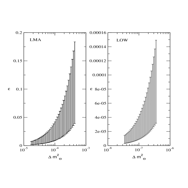
Figure 1: The range of $\epsilon$ as a function of $\Delta m_{\odot}^{2}$ corresponding to the 99% C.L. range of allowed values of $\Delta m_{atm}^{2}$ and $\sin^{2}2\theta_{atm}$ from [11]. The $\Delta m_{\odot}^{2}$ shown corresponds to the 99% C.L. allowed range for LMA (left hand panel) and LOW (right hand panel) solutions from [12].

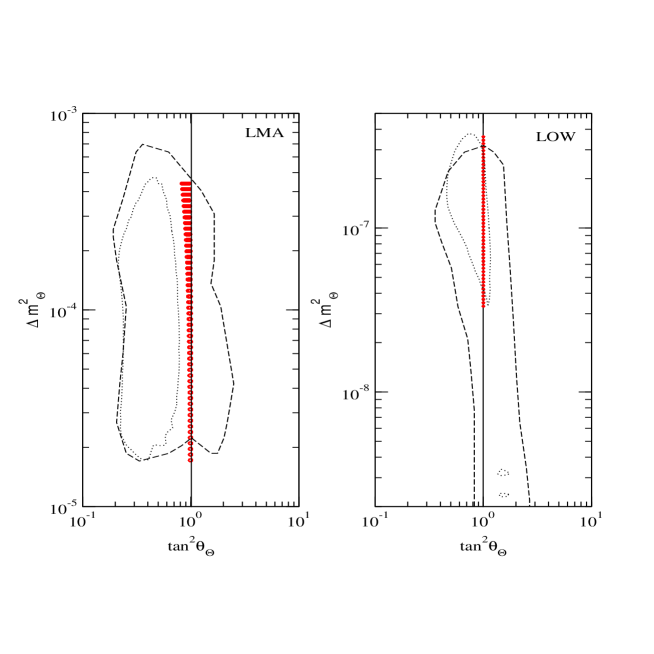
Figure 2: Comparison of the Zee model predictions with the allowed parameter values from the current experimental data. Values of $\tan^{2}\theta_{\odot}$ and $\Delta m_{\odot}^{2}$ predicted by the Zee model are shown by the red horizontal errorbars. The dotted lines give the 99% C.L. allowed areas in the LMA (left hand panel) and LOW (right hand panel) regions from the analysis of [12]. The dashed lines give corresponding allowed zones at 99% C.L. from the analysis of Bahcall et al [14].

References

- [1] A. Zee, Phys. Lett. B93, 389 (1980); Phys. Lett. B 161, 141 (1985); L. Wolfenstein, Nucl. Phys. B175, 93 (1980); S. T. Petcov, Phys. Lett. B115, 401 (1982).
- [2] A. Yu. Smirnov and M. Tanimoto, Phys. Rev. D55, 1665 (1997)
- [3] C. Jarlskog, M. Matsuda, S. Skadhauge, M. Tanimoto, Phys. Lett. B449, 240 (1999)
- [4] S.T. Petcov, Phys. Lett. B110, 245 (1982).
- [5] P. H. Frampton, S. L. Glashow, Phys. Lett. B461, 95 (1999)
- [6] E. Mitsuda, K. Sasaki, Phys. Lett. B516 47 (2001); A. Ghosal, Y. Koide, H. Fusaoka, Phys. Rev. D64, 053012 (2001); K.R.S. Balaji, W. Grimus, T. Schwetz, Phys. Lett. B508 301 (2001); Y. Koide, A. Ghosal, Phys. Rev. D63, 037301 (2001); N. Gaur, A. Ghosal, E. Ma, P. Roy, Phys. Rev. D58 071301 (1998); S. Kanemura, T. Kasai, G. L. Lin, Y. Okada, J.-J. Tseng, C.P. Yuan Phys. Rev. D64, 053007 (2001); K. Cheung, O. C.W. Kong, Phys. Rev. D61, 113012 (2000); A. Yu. Smirnov, Z-j Tao, Nucl. Phys. B426, 415 (1994).
- [7] Y. Koide, Phys. Rev. D64, 077301 (2001).
- [8] P. H. Frampton, M. C. Oh, T. Yoshikawa, e-Print Archive: hep-ph/0110300
- [9] B. Pontecorvo, Zh. Eksp. Teor. Fiz. 33, 549 (1957); 34, 247 (1958); Z. Maki, N. Nakagawa, S. Sakata, Prog. Theor. Phys. 28, 870 (1962).
- [10] M. Appolonio et al., Phys. Lett. B466, 415 (1999); Phys. Lett. B420, 397 (1998).
- [11] G.L.Fogli, E.Lisi, A. Marrone, e-Print Archive: hep-ph/0110089.
- [12] A. Bandyopadhyay, S. Choubey, S. Goswami , K. Kar, Phys. Lett. B519, 83 (2001).
- [13] G.L. Fogli, E. Lisi, D. Montanino, A. Palazzo, Phys. Rev. D64, 093007 (2001); P.I. Krastev and A.Yu. Smirnov, e-Print Archive: hep-ph/0108177; M.V. Garzelli and C. Giunti, e-Print Archive: hep-ph/0108191.
- [14] J.N. Bahcall, M.C. Gonzalez-Garcia, C. Pana-Garay, JHEP 0108, 014 (2001).
- [15] M.C. Gonzalez-Garcia, C. Pana-Garay, Y. Nir , A.Yu. Smirnov, Phys. Rev. D63, 013007 (2001).
- [16] S. Choubey, S. Goswami, D.P. Roy, e-Print Archive: hep-ph/0109017, to appear in Phys. Rev. D.