Wave functions and spectra from (S)DLCQ

Abstract

Applications of discretized light-cone quantization (DLCQ) to (3+1)-dimensional Yukawa theory with Pauli–Villars regulators and of supersymmetric DLCQ (SDLCQ) to (2+1)-dimensional super Yang–Mills theory are discussed. The ability of these methods to provide wave functions as well as spectra is emphasized.

1 INTRODUCTION

To be able to fully describe hadrons from first principles in quantum chromodynamics (QCD), one needs to be able to compute wave functions and spectra. Progress toward making such a computation in the context of light-cone quantization has been steady [1]. Two particular approaches will be discussed here. Both make use of the discretized light-cone quantization (DLCQ) technique pioneered by Pauli and Brodsky [2] for the numerical solution of quantum field theories. The approaches differ in how the theory is regulated; one uses Pauli–Villars (PV) regularization [3] and the other supersymmetry.

The use of PV regularization with DLCQ in (3+1)-dimensional theories has been developed by Brodsky, Hiller, and McCartor [4, 5, 6]. The initial work involved simple many-body models [4, 5]. New work discussed here and elsewhere [6] is for Yukawa theory in a single-fermion truncation. The essential idea is to include PV particles in the DLCQ basis. Cancellation of ultraviolet infinities is then arranged by choosing imaginary couplings or an indefinite metric. In the case of Yukawa theory there are choices to be made about the particle content of the PV sector. The work to be discussed here used three heavy scalars, two of which have negative norm. An alternative now under investigation is to use one heavy scalar and one heavy fermion, both with negative norm. This alternative was suggested by the work of Paston et al. [7] and has the advantage of being free of instantaneous fermion interactions.

Supersymmetric theories are simpler with respect to regularization but require greater care in the numerical discretization. A key insight to the correct discretization was made by Matsumura, Sakai, and Sakai [8]. They noticed that by discretizing the supercharge $Q^{-}$ and constructing a discrete light-cone energy $P^{-}$ from the superalgebra, one could retain supersymmetry in the discrete approximation, now called SDLCQ [9]. Ordinary DLCQ discretizes $P^{-}$ directly and recovers supersymmetry only in the infinite resolution limit. The SDLCQ technique has been refined and applied by Pinsky and collaborators [9], initially in 1+1 dimensions, but now also in 2+1 dimensions [10, 11]. Recent work on (2+1)-dimensional supersymmetric Yang–Mills theory is discussed here and elsewhere [11, 12].

Both approaches rely on DLCQ. All light-cone momentum variables are discretized, with $p^{+}\rightarrow n\pi/L$ and $\vec{p}_{\perp}\rightarrow\vec{n}_{\perp}\pi/L_{\perp}$, in terms of longitudinal and transverse length scales $L$ and $L_{\perp}$. The integrals over wave functions that make up the mass eigenvalue problem $H_{\rm LC}\Phi=M^{2}\Phi$ are then approximated by the trapezoidal quadrature rule. This yields a matrix eigenvalue problem which is typically quite large but also quite sparse. Lanczos techniques [13] are used to extract eigenvalues and eigenvectors for the lowest states, even in the case of an indefinite metric [6].

Because the longitudinal momentum is always positive, there exists a positive integer $K$, called the (harmonic) resolution [2], such that the total longitudinal momentum is $P^{+}=K\pi/L$ and momentum fractions are given by $x=n/K$. Wave functions and the mass eigenvalue problem, where $H_{\rm LC}=P^{+}P^{-}$, are naturally expressed in terms of momentum fractions and the resolution $K$. Hence $L$ disappears, and $K$ effectively takes its place as the resolution scale. The transverse scale $L_{\perp}$ is set by a momentum cutoff and a transverse resolution.

The remainder of this paper contains brief discussions of recent work on Yukawa theory [6] in Sec. 2 and super Yang–Mills theory [11] in Sec. 3. A summary and discussion of future work are given in Sec. 4.

2 YUKAWA THEORY

When terms involving antifermions are eliminated, the Yukawa light-cone Hamiltonian becomes [14]

$$H_{\rm LC}=\sum_{\underline{n},s}\frac{M^{2}+\delta M^{2}+(\vec{n}_{\perp}\pi/L_{\perp})^{2}}{n/K}b_{\underline{n},s}^{\dagger}b_{\underline{n},s}$$

$$+\sum_{\underline{m}}\frac{\mu^{2}+(\vec{m}_{\perp}\pi/L_{\perp})^{2}}{m/K}a_{\underline{m}}^{\dagger}a_{\underline{m}}$$

$$+\frac{g\sqrt{\pi}}{2L_{\perp}^{2}}\sum_{\underline{n}\underline{m}s}\frac{1}{\sqrt{m}}\left[\frac{\vec{\epsilon}_{-2s}^{\,*}\cdot\vec{n}_{\perp}}{n/K}\right.$$

$$+\left.\frac{\vec{\epsilon}_{2s}\cdot(\vec{n}_{\perp}+\vec{m}_{\perp})}{(n+m)/K}\right]b_{\underline{n}+\underline{m},-s}^{\dagger}b_{\underline{n},s}a_{\underline{m}}$$

$$\rule{36.135pt}{0.0pt}+\mbox{h.c.}$$

$$+\frac{Mg}{\sqrt{8\pi}L_{\perp}}\sum_{\underline{n}\underline{m}s}\frac{1}{\sqrt{m}}\left[\frac{1}{n/K}\right.$$

$$+\left.\frac{1}{(n+m)/K}\right]b_{\underline{n}+\underline{m},s}^{\dagger}b_{\underline{n},s}a_{\underline{m}}+\mbox{h.c.}$$

$$+\frac{g^{2}}{8\pi L_{\perp}^{2}}\sum_{\underline{n}\underline{m}\underline{m}^{\prime}s}\frac{1}{\sqrt{mm^{\prime}}}$$

$$\times\left[b_{\underline{n}+\underline{m}+\underline{m}^{\prime},s}^{\dagger}b_{\underline{n},s}a_{\underline{m}^{\prime}}a_{\underline{m}}\frac{1}{(n+m)/K}+\mbox{h.c.}\right.$$

$$+b_{\underline{n}+\underline{m}-\underline{m}^{\prime},s}^{\dagger}b_{\underline{n},s}a_{\underline{m}^{\prime}}^{\dagger}a_{\underline{m}}$$

$$\left.\times\left(\frac{1}{(n-m^{\prime})/K}+\frac{1}{(n+m)/K}\right)\right]$$

where

$$\left\{b_{\underline{n},s},b_{\underline{n}^{\prime},s^{\prime}}^{\dagger}\right\} = \delta_{\underline{n},\underline{n}^{\prime}}\delta_{s,s^{\prime}}\,,$$ (2)

$$\left[a_{\underline{m}},a_{\underline{m}^{\prime}}^{\dagger}\right] = \delta_{\underline{m},\underline{m}^{\prime}}\,,$$

and

$$\vec{\epsilon}_{\lambda}=-\frac{1}{\sqrt{2}}(\lambda,i)\,.$$ (3)

The one-loop contribution to the fermion self energy is [4]

$$I(\mu^{2},M^{2})\simeq\frac{\pi}{\mu^{2}}\left[\left(\frac{\Lambda^{2}}{2}-\mu^{2}\ln\Lambda^{2}\right.\right.$$

$$\rule{72.26999pt}{0.0pt}\left.+\mu^{2}\ln\mu^{2}-\frac{\mu^{4}}{2\Lambda^{2}}\right)$$

$$+M^{2}\left(3\ln\Lambda^{2}-3\ln\mu^{2}-\frac{9}{2}+\frac{5\mu^{2}}{\Lambda^{2}}\right)$$

$$+\left.M^{4}\left(\frac{2}{\mu^{2}}\ln(M^{2}/\mu^{2})+\frac{1}{3\mu^{2}}-\frac{1}{2\Lambda^{2}}\right)\right]\,,$$

with $\Lambda$ a cutoff. For this to be finite and consistent with zero in the $M\rightarrow 0$ chiral limit, we need to perform three subtractions. Therefore we add to the Hamiltonian three heavy PV scalars [15] with masses $\mu_{i}$ and couplings $\xi_{i}g$ determined by

$$1+\sum_{i=1}^{3}(-i)^{i}\xi_{i}=0\,,\;\;\mu^{2}+\sum_{i=1}^{3}(-i)^{i}\xi_{i}\mu_{i}^{2}=0\,,$$ (5)

$$\sum_{i=1}^{3}(-i)^{i}\xi_{i}\mu_{i}^{2}\ln(\mu_{i}^{2}/\mu^{2})=0\,.$$

These constraints guarantee the desired one-loop subtractions if the norm of the i-th PV boson is $(-1)^{i}$. Fermion self-induced inertia terms have not been included because they cancel once the heavy scalars are added.

The state vector is

$$\Phi_{\sigma}=\sqrt{16\pi^{3}P^{+}}\sum_{n_{0},n_{1},n_{2},n_{3}=0}^{\infty}\int\frac{dp^{+}d^{2}p_{\perp}}{\sqrt{16\pi^{3}p^{+}}}$$

$$\times\prod_{j=1}^{n_{\rm tot}}\int\frac{dq_{j}^{+}d^{2}q_{\perp j}}{\sqrt{16\pi^{3}q_{j}^{+}}}\sum_{s}\delta(\underline{P}-\underline{p}-\sum_{j}^{n_{\rm tot}}\underline{q}_{j})$$

$$\times\phi_{\sigma s}^{(n_{i})}(\underline{q}_{j};\underline{p})\frac{1}{\sqrt{\prod_{i}n_{i}!}}b_{\underline{p}s}^{\dagger}\prod_{j}^{n_{\rm tot}}a_{i_{j}\underline{q}_{j}}^{\dagger}|0\rangle\,,$$

with $n_{\rm tot}=\sum_{i}n_{i}$ and normalization

$$\Phi_{\sigma}^{\prime\dagger}\cdot\Phi_{\sigma}=16\pi^{3}P^{+}\delta(\underline{P}^{\prime}-\underline{P})\,.$$ (7)

To cancel an infrared singularity in the instantaneous fermion term, we add an effective interaction that represents the contribution of the missing Z graph. The added term is built diagrammatically from the pair production and annihilation terms

$${\cal P}_{\rm pair}^{-}=\frac{g}{2L_{\perp}\sqrt{L}}\sum_{\underline{p}\underline{q}si}\left[\frac{\vec{\epsilon}_{-2s}\cdot\vec{p}_{\perp}}{p^{+}\sqrt{q^{+}}}\right.$$

$$+\left.\frac{\vec{\epsilon}_{2s}^{\,*}\cdot(\vec{q}_{\perp}-\vec{p}_{\perp})}{(q^{+}-p^{+})\sqrt{q^{+}}}\right]b_{\underline{p},s}^{\dagger}d_{\underline{q}-\underline{p},s}^{\dagger}\xi_{i}a_{i\underline{q}}+\mbox{h.c.}$$

$$+\frac{Mg}{2L_{\perp}\sqrt{2L}}\sum_{\underline{p}\underline{q}si}\left[\frac{1}{p^{+}\sqrt{q^{+}}}\right.$$

$$-\left.\frac{1}{(q^{+}-p^{+})\sqrt{q^{+}}}\right]b_{\underline{p},s}^{\dagger}d_{\underline{q}-\underline{p},-s}^{\dagger}\xi_{i}a_{i\underline{q}}+\mbox{h.c.}\,,$$

and the denominator for the intermediate state

$$\frac{M^{2}}{P^{+}} - p_{\rm spectators}^{-}-\frac{M^{2}+p_{\perp}^{\prime 2}}{p^{\prime+}}$$

$$- \frac{M^{2}+(\vec{q}_{\perp}^{\,\prime}-\vec{p}_{\perp})^{2}}{q^{\prime+}-p^{+}}-\frac{M^{2}+p_{\perp}^{2}}{p^{+}}\,.$$

The bare parameters of the Hamiltonian, $g$ and $\delta M^{2}$, are determined by input of “data.” The mass $M$ of the dressed single-fermion state is held fixed. This is imposed by rearranging the mass eigenvalue problem into an eigenvalue problem for $\delta M^{2}$:

$$x\left[M^{2}-\frac{M^{2}+p_{\perp}^{2}}{x}-\sum_{j}\frac{\mu_{j}^{2}+q_{\perp j}^{2}}{y_{j}}\right]\tilde{\phi}$$

$$-\int\prod_{j}dy^{\prime}_{j}d^{2}q^{\prime}_{\perp j}\sqrt{xx^{\prime}}{\cal K}\tilde{\phi}^{\prime}=\delta M^{2}\tilde{\phi}\,,$$

where ${\cal K}$ represents the original kernel and amplitudes are related by $\phi=\sqrt{x}\tilde{\phi}$.

To fix the coupling we use $\langle:\!\!\phi^{2}(0)\!\!:\rangle\equiv\Phi_{\sigma}^{\dagger}\!:\!\!\phi^{2}(0)\!\!:\!\Phi_{\sigma}$. From a numerical solution it can be computed fairly efficiently in a sum similar to the normalization sum

$$\langle:\!\!\phi^{2}(0)\!\!:\rangle=\sum_{n_{i}=0}^{\infty}\int\prod_{j}^{n_{\rm tot}}\,dq_{j}^{+}d^{2}q_{\perp j}\sum_{s}(-1)^{(n_{i})}$$

$$\times\left(\sum_{k=1}^{n}\frac{2}{q_{k}^{+}/P^{+}}\right)\left|\phi_{\sigma s}^{(n_{i})}(\underline{q}_{j};\underline{P}-\sum_{j}\underline{q}_{j})\right|^{2}\,.$$

The constraint on $\langle:\!\!\phi^{2}(0)\!\!:\rangle$ is satisfied by solving it simultaneously with the eigenvalue problem.

With the parameters fixed, we can compute various quantities. Those considered include structure functions, the form factor slope at zero momentum transfer, average numbers of constituents, and average constituent momenta. A representative plot of the bosonic structure function

$$f_{B}(y)\equiv\sum_{n_{i}=0}^{\infty}\sum_{s}\int\,\prod_{j}dq_{j}^{+}d^{2}q_{\perp j}(-1)^{(n_{i})}\sum_{k=1}^{n_{0}}$$ (12)

$$\times\delta(y-q_{k}^{+}/P^{+})\left|\phi_{\sigma s}^{(n_{i})}(\underline{q}_{j};\underline{P}-\sum_{i}\underline{q}_{j})\right|^{2}\,,$$

is given in Fig. 1.

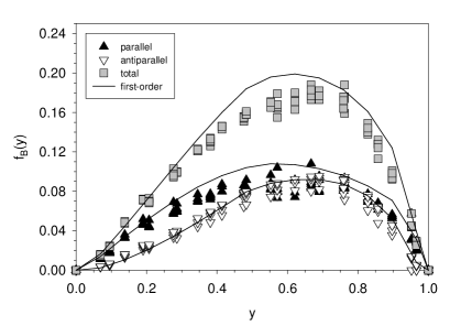
Figure 1: The boson structure function $f_{B}$ at various numerical resolutions for $\langle:\!\!\phi^{2}(0)\!\!:\rangle=0.5$, with $M=\mu$, cutoff $\Lambda^{2}=50\mu^{2}$, and Pauli–Villars masses $\mu_{1}^{2}=10\mu^{2}$, $\mu_{2}^{2}=20\mu^{2}$, and $\mu_{3}^{2}=30\mu^{2}$. The solid line is from first-order perturbation theory.

Additional results can be found in Ref. [6]. For good results at stronger couplings, where first-order perturbation theory is insufficient, rather high resolution was required, with $K=21$ to 39 and as many as 15 transverse momentum points. This resolution was achieved by limiting the number of constituents to 3, after verifying that the contribution from higher sectors was sufficiently small.

3 SUPER YANG–MILLS THEORY

The Lagrangian for supersymmetric SU(N) Yang–Mills theory in 2+1 dimensions is

$${\cal L}=\mbox{tr}(-\frac{1}{4}F^{\mu\nu}F_{\mu\nu}+{\rm i}{\bar{\Psi}}\gamma^{\mu}D_{\mu}\Psi)\,,$$ (13)

where $F_{\mu\nu}=\partial_{\mu}A_{\nu}-\partial_{\nu}A_{\mu}+ig[A_{\mu},A_{\nu}]$ and $D_{\mu}\Psi=\partial_{\mu}\Psi+ig[A_{\mu},\Psi]$. We work in light-cone gauge ($A^{+}=0$) and the large-$N$ limit. The dynamical fields are $\phi\equiv A_{2}$ and $\psi\equiv 2^{-1/4}(1+\gamma^{5})\Psi$. The supercharge $Q^{-}$ is

$$Q^{-}=2^{3/4}\int dx^{-}\int_{0}^{l}dx_{\perp}\mbox{tr}\left[\partial_{\perp}\phi\psi\right.$$ (14)

$$+\left.g_{\rm YM}\left({\rm i}[\phi,\partial_{-}\phi]+2\psi\psi\right)\frac{1}{\partial_{-}}\psi\right]\,.$$

and $P^{-}$ is given by $\{Q^{-},Q^{-}\}=2\sqrt{2}P^{-}$. By discretizing $Q^{-}$ and computing $P^{-}$ from this anticommutator, supersymmetry is exactly preserved in the numerical approximation [8]. In addition to supersymmetry, we have transverse parity and the Kutasov $T$ symmetry [16]. The mass eigenvalue problem can then be solved separately in each of the 8 symmetry sectors. In the largest calculation to date [11], each sector contained roughly 230,000 basis states.

A variety of results can be seen in Ref. [11]. They include a number of studies of the coupling dependence of the mass values, as well as outcomes for structure functions. One striking feature is that, except for weak coupling, the average particle count for almost all eigenstates is at or near the maximum allowed by the resolution, even for the highest resolution considered. This means that for strong coupling the method does not capture all of the important pieces of the true eigenstate. Such behavior is likely to be a consequence of dealing with massless constituents without introducing a mass scale through symmetry breaking or other means.

Another striking feature is that the average number of fermions in bosonic states has been observed to have a gap between 4 and 6. This could only be checked for resolutions where a full diagonalization could be done. However, as can be seen in Fig. 2, the signal is quite clean for $K=6$ and 3 transverse momentum modes, where the average number is never above 4 unless it is precisely 6, the maximum allowed; below 4 there are no gaps at all.

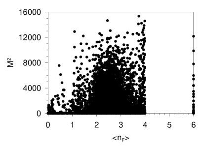
Figure 2: Bound-state masses squared $M^{2}$ in units of $4\pi^{2}/L_{\perp}^{2}$ for bosonic states as functions of the average number of fermions $\langle n_{F}\rangle$ for $K=6$. Several different values of the coupling are included. The symmetry sector is one with positive $T$ symmetry and positive parity.

4 FUTURE WORK

Both ordinary DLCQ with Pauli–Villars particles and SDLCQ provide the means to compute masses and wave functions for eigenstates in multi-dimensional quantum field theories. These methods will continue to be explored in various contexts, leading eventually to consideration of (supersymmetric) QCD. In fact, Paston et al. [17] have already obtained a PV-like regularization of QCD that could, in principle, be solved by DLCQ; however, with present computing power the number of fields is probably too large for meaningful calculations.

With QCD as a goal, work on the PV approach will next turn to the alternative regularization of Yukawa theory, with one heavy scalar and one heavy fermion [7], in both the one and two-fermion Fock sectors. Quantum electrodynamics will also be considered, as a first application to a gauge theory and as something of interest in its own right.

The next step for work with SDLCQ is to include a Chern–Simons term in super Yang–Mills theory and thereby give each constituent a nonzero mass. The extension of the method to 3+1 dimensions is also important, as is consideration of supersymmetry breaking.

References

• [1] S.J. Brodsky, H.C. Pauli, and S.S. Pinsky, Phys. Rep. 301 (1997) 299; Nucl. Phys. B (Proc. Suppl.) 90 (2000) 170, hep-ph/0007309.
• [2] H.-C. Pauli and S.J. Brodsky, Phys. Rev. D 32 (1985) 1993; 32 (1985) 2001.
• [3] W. Pauli and F. Villars, Rev. Mod. Phys. 21 (1949) 4334.
• [4] S.J. Brodsky, J.R. Hiller, and G. McCartor, Phys. Rev. D 58 (1998) 025005, hep-th/9802120.
• [5] S.J. Brodsky, J.R. Hiller, and G. McCartor, Phys. Rev. D 60 (1999) 054506, hep-ph/9903388.
• [6] S.J. Brodsky, J.R. Hiller, and G. McCartor, to appear in Phys. Rev. D, hep-ph/0107038.
• [7] S.A. Paston, E.V. Prokhvatilov, and V.A. Franke, hep-th/9910114.
• [8] Y. Matsumura, N. Sakai, and T. Sakai, Phys. Rev. D 52 (1995) 2446.
• [9] O. Lunin and S. Pinsky, in the proceedings of 11th International Light-Cone School and Workshop: New Directions in Quantum Chromodynamics and 12th Nuclear Physics Summer School and Symposium (NuSS 99), Seoul, Korea, 26 May - 26 Jun 1999 (New York, AIP, 1999), p. 140, hep-th/9910222.
• [10] F. Antonuccio, O. Lunin, and S. Pinsky, Phys. Rev. D 59 (1999) 085001, hep-th/9811083; P. Haney, J. R. Hiller, O. Lunin, S. Pinsky, and U. Trittmann Phys. Rev. D 62 (2000) 075002, hep-th/9911243; J.R. Hiller, S.S. Pinsky, and U. Trittmann, Phys. Rev. D 63 (2001) 105017, hep-th/0101120.
• [11] J.R. Hiller, S.S. Pinsky, and U. Trittmann, Phys. Rev. D 64 (2001) 105027, hep-th/0106193.
• [12] See contributions to this volume by U. Trittmann and S. Pinsky.
• [13] C. Lanczos, J. Res. Nat. Bur. Stand. 45, 255 (1950); J.H. Wilkinson, The Algebraic Eigenvalue Problem (Clarendon, Oxford, 1965); B.N. Parlett, The Symmetric Eigenvalue Problem (Prentice–Hall, Englewood Cliffs, NJ, 1980); J. Cullum and R.A. Willoughby, J. Comput. Phys. 44, 329 (1981); Lanczos Algorithms for Large Symmetric Eigenvalue Computations (Birkhauser, Boston, 1985), Vol. I and II; G.H. Golub and C.F. van Loan, Matrix Computations (Johns Hopkins University Press, Baltimore, 1983).
• [14] G. McCartor and D.G. Robertson, Z. Phys. C 53 (1992) 679.
• [15] C. Bouchiat, P. Fayet, and N. Sourlas, Lett. Nuovo Cim. 4 (1972) 9; S.-J. Chang and T.-M. Yan, Phys. Rev. D 7 (1973) 1147; M. Burkardt and A. Langnau, Phys. Rev. D 44 (1991) 3857.
• [16] D. Kutasov, Nucl. Phys. B 414 (1994) 33.
• [17] S.A. Paston, V.A. Franke, and E.V. Prokhvatilov, Theor. Math. Phys. 120 (1999) 1164, hep-th/0002062. See also the contribution to this volume.