Direct Photons from Relativistic Heavy-Ion Collisions

Abstract

Direct photons have been proposed as a promising signature for the quark-gluon plasma (QGP) formation in relativistic heavy-ion collisions. Recently WA98 presented the first data on direct photons in $Pb$+$Pb$-collisions at SPS. At the same time RHIC started with its experimental program. The discovery of the QGP in these experiments relies on a comparison of data with theoretical predictions for QGP signals. In the case of direct photons new results for the production rates of thermal photons from the QGP and a hot hadron gas as well as for prompt photons from initial hard parton scatterings have been proposed recently. Based on these rates a variety of different hydrodynamic models, describing the space-time evolution of the fireball, have been adopted for calculating the direct photon spectra. The results have been compared to the WA98 data and predictions for RHIC and LHC have been made. So far the conclusions of the various models are controversial.

The aim of the present review is to provide a comprehensive and up-to-date survey and status report on the experimental and theoretical aspects of direct photons in relativistic heavy-ion collisions.

1 Introduction

The major motivation to study relativistic heavy-ion collisions is the search for the quark-gluon plasma (QGP), a potential new state of matter where colored quarks and gluons are no longer confined into hadrons and chiral symmetry is restored. The phase transition to quark matter has been predicted first for the interior of neutron stars [1, 2] and afterwards in high-energy nucleus-nucleus collisions [3, 4, 5]. Subsequently it has been studied in great detail in lattice QCD [6]. The quark-gluon plasma phase could provide insight in the important non-perturbative features that usually govern hadronic physics.

A wealth of knowledge has been accumulated by the early experiments especially at the CERN SPS accelerator (see e.g. [7, 8]). Many of the properties of these collisions have been studied and interesting observations have been made concerning non-trivial behavior of the strongly interacting matter, most notably the suppression of J/$\psi$ production beyond the expectation from normal nuclear effects, the enhancement of strangeness production, modifications of the dilepton spectrum and direct photon production in excess of known extrapolations from particle physics. Some of these observations were actually predicted to happen in relation to the phase transition to a QGP, and one possible conclusion, guided by Ockham’s razor, is to see the experimental hints as evidence, though “circumstantial”, of the new phase [9].

However, a real understanding of the related physical concepts is extremely difficult. Not only are most of the involved processes soft, and thereby in the domain of large coupling constants where perturbation theory breaks down, but the system itself is a multi-particle system, which is already a challenge in situations where the underlying interaction is much weaker. Although one might hope that in large enough nuclei the system might be governed at least partially by laws of thermodynamics, and thus be treatable, the conditions are complicated further by the need to control the residual non-equilibrium aspects.

To study such a complicated system one wishes for a probe that is not equally complicated in itself. The production of hadrons is of course governed by the strong interaction and therefore adds to the complication. One possible way out might be the study of hard processes where QCD, the theory of strong interaction, enters the perturbative regime and is calculable. The other avenue involves a particle that suffers only electromagnetic interaction: Photons — both real and virtual — should be an ideal probe. As we will discuss in the present report, while photon production may be less difficult to treat than some other processes in hadronic physics, an adequate treatment in heavy-ion collisions turns out to be far from trivial. Experimentally, high energy direct photon measurement has always been considered a challenge. This is true already in particle physics and even more in the environment of heavy-ion collisions. Nevertheless a lot of progress has been made and a large amount of experimental data is available, though mostly from particle physics. Direct photon measurements in heavy-ion collisions are expected to come into real fruition with the advent of colliders like RHIC and LHC.

In the present report we attempt to provide a comprehensive review of the theoretical and experimental aspects of the study of direct photon production in heavy-ion collisions. We will also touch photon production in proton-proton collisions as far as we consider it relevant to our main subject. Because of the large amount of work existing, we will most likely not be able to do justice to all of it, and we would like to apologize for any omission or mistreatment of related publications.

The structure of the present report will be as follows: In the next Section we will discuss the theoretical status of the photon production from $pp$ to $AA$ collisions. In particular, we will consider the calculation of the rates from the QGP, from the hot hadron gas, and from initial hard collisions. Furthermore, we review some basics of the hydrodynamical description for deriving photon spectra in heavy-ion collisions. In Section 3 experimental concepts for measuring direct photons and results from $pp$ and $pA$ collisions as well as from ${}^{16}O$-, ${}^{32}S$- and ${}^{208}Pb$-induced reactions are reviewed. In Section 4 these results are compared to theoretical calculations, and predictions for RHIC and LHC are presented. The following summary will conclude this review. Appendix A and B provide some technical details for calculating the photon production rate from the QGP.

2 Theoretical Status

The theoretical prediction and calculation of the photon emission, i.e. yields and spectra, from a thermal system has a long tradition, culminating in the discovery of quantum physics [12]. In astrophysics the detection of electromagnetic radiation from the hot surfaces of stars and other objects, even from the entire universe (Cosmic Microwave Background), provides the most essential information, such as temperature, size, chemical composition etc. In particular deviations from the pure black-body spectrum are of utmost interest, e.g. to learn about the composition, evolution, and structure formation in the universe from the Cosmic Microwave Background [13].

The photon emission from the nuclear fireball, created in a relativistic heavy-ion collision, differs from the one of macroscopic stellar objects in the following respect. Whereas the photons in the latter case are thermalized when they leave the surface, the mean-free path of the photons produced in nucleus-nucleus collisions is large compared to the size of the fireball. Hence, the photons do not interact after their production and leave the fireball undisturbed. As a consequence they carry information about the stage of the fireball at the time of their creation. The photon spectrum, containing photons from all stages, allows therefore to study the entire evolution of the fireball. Direct photons, together with dileptons and to some extent hard probes like jet quenching, are therefore a unique diagnostic tool for the different phases and the equation of state (EOS) of the ultradense matter produced in high-energy nuclear collisions. Photon production in high-energy nuclear and particle physics provides information on the momentum distributions of the emitting particles. In particle physics this may be used to extract information on structure functions. In thermalized systems, expected in nuclear collisions, it should yield information on the thermal distributions.

To draw conclusions about the state of the matter in the fireball, created in relativistic heavy-ion collisions, it is necessary to compare the experimental data for direct photons with theoretical calculations. The ideal theoretical description would be a comprehensive treatment of the entire space-time evolution of the fireball from the first contact of the cold nuclei to the freeze-out and subsequent decay of hadrons, e.g. in a dynamical lattice QCD approach. At the same time all participating particle species and their interactions should be included. Due to the complexity of the problem, e.g. the consistent treatment of hadronization and the non-perturbative nature of the strong interaction, such a systematic investigation is presently only wishful thinking. Alternatively, the different stages of the fireball (initial stage, pre-equilibrium QGP, thermal QGP, mixed phase and hadronization, hot hadron gas, freeze-out and hadronic decays) are treated separately. Furthermore, one computes first the production rates of the photons from the different stages, e.g. at a given temperature. Then these rates are convoluted with the space-time evolution of the fireball using mostly hydrodynamical models. In this way, estimates of the photon spectra are obtained, which can be compared to experimental results.

In the present chapter we will discuss in detail the status and problems of calculating production rates of direct photons from a thermal QGP and hadron gas as well as from hard scatterings in the initial non-equilibrium stage. In addition, the various hydrodynamical approaches and their applications to photon spectra will be critically reviewed.

2.1 Photon Production Rates

In this Section the calculation of the production rates of direct photons with experimentally relevant energies $E\gg T$ from a thermal QGP, a hot hadron gas (HHG) and of prompt photons from the initial phase will be considered. Since direct photons have been proposed as a promising signature of the QGP formation in relativistic heavy-ion collisions [15, 16, 17, 18, 19, 20, 21, 22], emphasis is put on the photon production from the QGP and the calculation of this rate will be discussed first in detail.

Particle production rates can be computed from the amplitudes of the basic processes for the particle production, convoluted with the distribution functions of the participating particles [23]. For example, the production rate of a particle $A$ with energy $E$ follows from

$$\Gamma_{\rm prod}(E)=\frac{1}{2E}\int\frac{d^{3}p_{1}}{(2\pi)^{3}2E_{1}}...\frac{d^{3}p_{m}}{(2\pi)^{3}2E_{m}}\>\frac{d^{3}p^{\prime}_{1}}{(2\pi)^{3}2E^{\prime}_{1}}...\frac{d^{3}p^{\prime}_{n}}{(2\pi)^{3}2E^{\prime}_{n}}$$

$$(2\pi)^{4}\>\delta(P-\sum_{i=1}^{m}P_{i}+\sum_{i=1}^{n}P^{\prime}_{i})\>\sum_{i,j}|\mathcal{M}|^{2}\>f_{1}...f_{m}\>(1\pm f^{\prime}_{1})...(1\pm f^{\prime}_{n}).$$ (1)

Here $\mathcal{M}$ is the matrix element of the basic process for the production of particle $A$, where $m$ particles participate in the initial and $n$ particles (denoted by a prime) in the final channel. $\sum_{i,j}$ indicates the sum over all states of the particles in the initial and final states except of the particle $A$, and $P$, $P_{i}$, and $P^{\prime}_{j}$ are the 4-momenta of the particles. $f_{i}$ denotes the distribution functions of the incoming particles and $f^{\prime}_{j}$ of the outgoing ones (except of $A$). For outgoing bosons, the plus sign holds, corresponding to Bose-enhancement, whereas for fermions the minus sign, corresponding to Pauli-blocking. In an equilibrated system, such as the QGP or the HHG, the distribution functions are given by Bose-Einstein or Fermi-Dirac distributions, respectively. In high-energy particle physics, such as the production of prompt photons in $pp$ collisions, the parton structure functions are taken.

2.1.1 Thermal Rates from the QGP

A QGP emits photons as every thermal source does. The microscopic process is the photon radiation from quarks having an electric charge. Due to energy-momentum conservation, these quarks have to interact with the thermal particles of the QGP in order to emit a photon. Hence, an ideal, non-interacting QGP cannot be seen. However, there will always be (strong and electromagnetic) interactions in the QGP, such as quark-antiquark annihilation. However, due to energy-momentum conservation the direct annihilation of quarks and anti-quarks into real photons is also not possible but only into virtual photons which can decay into lepton pairs. The production of dileptons is another promising signature for the QGP [24], which, however, is not the topic of the present review. To lowest order perturbation theory, real photons are produced from the annihilation of a quark-antiquark pair into a photon and a gluon ($q\bar{q}\rightarrow g\gamma$) and by absorption of a gluon by a quark emitting a photon ($qg\rightarrow q\gamma$), similar to Compton scattering in QED (see Fig. 1). A higher order process for the photon production is, for example, bremsstrahlung, where a quark radiates a photon by scattering off a gluon or another quark in the QGP.

Figure 1: Lowest order contributions to photon production from the QGP: Compton scattering (left) and quark-antiquark annihilation (right).

The photon production rate can be computed from the matrix elements of these basic processes by convoluting them with the distribution functions of the participating partons according to Eq. (1). In the case of processes with two partons in the initial and one in the final channel, such as annihilation and Compton scattering discussed above, the differential photon production rate is given by [25]

$$\frac{dN}{d^{4}xd^{3}p} = \frac{1}{(2\pi)^{3}2E}\>\int\frac{d^{3}p_{1}}{(2\pi)^{3}2E_{1}}\frac{d^{3}p_{2}}{(2\pi)^{3}2E_{2}}\frac{d^{3}p_{3}}{(2\pi)^{3}2E_{3}}\>n_{1}(E_{1})n_{2}(E_{2})[1\pm n_{3}(E_{3})]$$ (2)

$$\sum_{i}\langle|\mathcal{M}|^{2}\rangle\>(2\pi)^{4}\>\delta(P_{1}+P_{2}-P_{3}-P).$$

Here $P_{1}$ and $P_{2}$ are the 4-momenta of the incoming partons, $P_{3}$ of the outgoing parton, and $P$ of the produced photon. Throughout the paper we use the notation $P=(p_{0},{\bf p})$ and $p=|{\bf p}|$, which is convenient in thermal field theory. For on-shell particles, the energy is denoted by $p_{0}=E$. In equilibrium, the distribution functions $n_{i}(E_{i})$ are given by the Bose-Einstein distribution, $n_{B}(E_{i})=1/[\exp(E_{i}/T)-1]$, for gluons and by the Fermi-Dirac distribution, $n_{F}(E_{i})=1/[\exp(E_{i}/T)+1]$, for quarks, respectively. The factor $[1\pm n_{3}(E_{3})]$ describes Pauli-blocking (minus sign) in the case of a final-state quark or Bose-enhancement (plus sign) in the case of a final-state gluon. The factor $\langle|\mathcal{M}|^{2}\rangle$ is the matrix element of the basic process averaged over the initial states and summed over the final states. The $\sum_{i}$ indicates the sum over the initial parton states. The delta function, as usual, ensures energy-momentum conservation. The formula Eq. (2) can be extended easily to higher order processes, by integrating over the momenta of the additional external partons, taking into account also their distribution functions. The differential rate, defined above, determines the number of emitted photons with momentum ${\bf p}$ within the interval $[{\bf p},{\bf p}+d^{3}p]$ and energy $E=p$ from the space-time volume $d^{4}x$. The total rate follows from integrating over the photon momentum. The observable spectrum is obtained by integrating over the space-time volume, by using for instance a hydrodynamical model, describing the space-time evolution of the expanding QGP. The total photon yield results from an integration of the spectrum over the photon momentum.

An alternative definition of the differential photon production rate is based on the polarization tensor or photon self-energy. According to cutting rules extended from vacuum quantum field theory to finite temperature [23, 26, 27], the differential rate can be related to the imaginary part of the polarization tensor $\Pi_{\mu\nu}(P)$ on its mass shell ($p_{0}=E=p$) [28]

$$\frac{dN}{d^{4}xd^{3}p}=-\frac{1}{(2\pi)^{3}}\>\frac{1}{E}\>\frac{1}{{\exp(E/T)-1}}\>{\rm Im}\,{\Pi_{\mu}}^{\mu}(E).$$ (3)

This expression is exact to first order in the electromagnetic coupling $\alpha$ and to all orders in the strong coupling constant $\alpha_{s}=g^{2}/4\pi$. Therefore, it contains in contrast to the definition Eq. (2), which holds only for $2\rightarrow 2$ reactions, also higher order processes like bremsstrahlung if the photon self-energy is chosen accordingly. The lowest order annihilation and Compton processes correspond to a polarization tensor containing one quark loop and one internal gluon line as shown in Fig. 2. Cutting these diagrams reproduces the processes of Fig. 1 in an illustrative way.

Figure 2: 2-loop polarization tensor. The dashed lines indicate cuts through the diagrams, corresponding to the processes in Fig. 1.

Now we will discuss the various attempts for calculating the production rate of energetic photons ($E\gg T$) from an equilibrated QGP.

Pre-HTL rate: Before the invention of the Hard-Thermal-Loop (HTL) improved perturbation theory (see below), the QGP photon rates have been calculated using the perturbative matrix elements for the processes of Fig. 1 together with Eq. (2) [15, 16, 20, 22]. In Ref.[20], even bremsstrahlung has been considered in this way. The derivation of the differential production rate of energetic photons ($E\gg T$), produced by the processes of Fig. 1, is presented in Appendix A. In the case of two thermalized quark flavors with bare mass $m_{0}$ it is given by [25]

$$\frac{dN}{d^{4}xd^{3}p}=\frac{5}{18\pi^{2}}\>\alpha\>\alpha_{s}\>\frac{T^{2}}{E}\>e^{-E/T}\>\ln\frac{ET}{m_{0}^{2}},$$ (4)

where $ET\gg m_{0}^{2}$ has been assumed.

It was noted that there is a logarithmic infrared (IR) sensitivity, i.e. the rate diverges logarithmically if the mass of the exchanged quark in Fig. 1 tends to zero. Therefore, Kajantie and Ruuskanen argued [18] that the bare quark mass should be replaced by an effective thermal quark mass. This means that even the production of energetic photons is sensitive to in-medium effects of the QGP, since the exchange of soft quarks plays an important role in the production mechanism. A systematic treatment of in-medium effects is provided by the HTL resummation technique, discussed below. Kajantie and Ruuskanen [18] used an effective, temperature-dependent quark mass calculated from the quark self-energy in the high temperature limit as discussed in Appendix B. The result is [30, 31]: $m_{q}^{2}=g^{2}T^{2}/6$. For $g=1.5$ - $2.5$ corresponding to realistic values $\alpha_{s}\simeq 0.2$ - $0.5$, one gets $m_{q}=0.6$ - $1.0$ $T$. For typical temperatures of the QGP, e.g. $T=200$ MeV, the effective quark mass is much larger than the bare mass of up and down quarks ($m_{u,d}\simeq 5$ - $10$ MeV) and of the same order as the bare strange quark mass. Hence, neglecting in-medium effects, i.e. adopting the bare instead of the effective quark mass in Eq. (4), leads to an overestimation of the rate. In the weak coupling limit, in which perturbation theory holds, the logarithm in Eq. (4) has to be replaced now by $\ln(E/\alpha_{s}T)$, neglecting a constant of the order of 1. As we will see below, using the HTL technique, this result is the leading logarithm approximation for the rate.

1-loop HTL rate: Using only bare propagators (and vertices) as in Fig. 1 or Fig. 2 for gauge theories (QED, QCD) at finite temperature, problems such as IR divergent and gauge dependent results are encountered. A famous example is the so-called plasmon puzzle: the damping rate of a gluon with a long wavelength or small momentum in a QGP, called plasmon, has been calculated in different gauges and different results have been found. In particular, in covariant gauges a negative result was obtained, indicating a puzzling instability of the QGP in perturbation theory [32]. Braaten and Pisarski [33] argued that naive perturbation theory, using only bare propagators (and vertices), is incomplete at finite temperature. Higher-order diagrams, containing infinitely many loops, can contribute to the same order in the coupling constant. These diagrams can be taken into account by resumming a certain class of diagrams, the hard thermal loops (HTLs). These diagrams are 1-loop diagrams (self-energies and vertex corrections), where the loop momentum is hard, i.e. of the order of the temperature or larger. This approximation agrees with the high-temperature limit of these diagrams, which has been computed already some time ago in the case of the gluon and quark self-energy [30, 31, 34]. Resumming these self-energies within a Dyson-Schwinger equation leads to effective gluon and quark propagators, which describe the propagation of collective gluon and quark modes in the QGP. These effective propagators (and similar effective vertices) have to be used if the momentum of the propagator is soft, i.e. of the order $gT$. Otherwise a bare propagator is sufficient. In this way, gauge invariant results for physical quantities are obtained and their IR behavior is improved. In the case of the plasmon damping rate, Braaten and Pisarski derived a positive, gauge independent result by using HTL-resummed gluon propagators and vertices [35]. It is important to note, that the HTL-resummation technique relies on the weak coupling limit assumption, $g\ll 1$, which allows the separation of the soft scale $gT$ and the hard scale $T$. The HTL-resummed perturbation theory is exemplified in Appendix B, where the photon production rate is calculated in this way. For a review of the HTL-method and its application see [36, 37, 38, 39].

Figure 3: Photon self-energy containing a HTL-resummed quark propagator indicated by the filled circle. The energy and momentum of the resummed quark propagator are soft, i.e. smaller than the separation scale $q_{c}$, whereas the other quark momentum is hard due to energy-momentum conservation in the case of hard photons.

In the case of massless quarks, the hard photon production rate from the QGP is logarithmically IR divergent due to the exchange of a massless quark, as discussed above. Therefore, the bare quark propagator has to be replaced by a HTL-resummed one, defined in Fig. 43 of Appendix B. According to the rules of the Braaten-Pisarski method, this has to be done for soft quark momenta. Therefore, we decompose the rate in a soft and a hard contribution, introducing a separation scale for the quark momentum $gT\ll q_{c}\ll T$ [40]. For the soft contribution, we start from Eq. (3) and use the diagram shown in Fig. 3 as polarization tensor. This 1-loop diagram has a non-vanishing imaginary part since the effective quark propagator contains an infinite number of loops (see Fig. 43). Cutting this diagram through the filled circle reproduces the diagrams shown in Fig. 1, where the bare quark propagator is replaced by a resummed one. It is not necessary to dress both propagators or to use an effective quark-photon vertex since only one internal quark line can be soft due to energy-momentum conservation in the case of hard photons. The hard contribution follows from the pre-HTL result, replacing the bare quark mass by the separation scale $q_{c}$ (see Appendix A). The details of these calculations are presented in Appendix B. Adding up the soft and the hard contribution, the separation scale cancels. In this way Kapusta et al. [25] and independently Baier et al. [41] found

$$\frac{dN}{d^{4}xd^{3}p}\biggl{|}_{\rm 1-loop}=a\>\alpha\alpha_{s}\>e^{-E/T}\>\frac{T^{2}}{E}\>\ln\frac{0.2317E}{\alpha_{s}T},$$ (5)

where $a=0.0281$ for $N_{F}=2$ thermalized quark flavors and $a=0.0338$ for $N_{F}=3$, respectively. The result has been extended to finite baryon density by generalizing the HTL-resummation technique to finite quark chemical potential [42]. It is interesting to note that for finite $\mu$ one has to give up the Boltzmann approximation for the initial parton distributions in the hard contribution (see Appendix B). Otherwise there is no cancellation of the separation scale after adding the hard and the soft part. Therefore, the photon production rate at finite $\mu$ can be determined only numerically. For $|\mu/T|<1$, the factor $T^{2}$ in Eq. (5) has to be replaced to a good accuracy simply by $T^{2}+\mu^{2}/\pi^{2}$ [43].

The 1-loop HTL photon production rate has also been calculated for a chemically non-equilibrated QGP [44, 45, 46, 47, 48], as discussed at the end of Section 2.2.1.

2-loop HTL rate: Naively one expects that higher order diagrams such as bremsstrahlung will contribute only to order $\alpha\,\alpha_{s}^{2}$. However, recently Aurenche et al. [49] showed that the 2-loop HTL contribution to the hard photon production rate is of order $\alpha\,\alpha_{s}$, i.e. contributes to Eq. (5) beyond the leading logarithm approximation. In the following, we will only sketch the arguments without presenting the calculation in detail.

The 1-loop HTL contribution of Fig. 3 to the hard photon production rate corresponds to the exchange of a soft, collective quark. The logarithmic IR singularity in the case of massless bare quarks is cut off by medium effects (in-medium quark “mass”) of the order $gT$. The complete second order HTL rate follows from adding the 1-loop HTL contribution for soft quarks and the 2-loop diagram of Fig. 2, where the intermediate quark is hard. Note that in Fig. 2 we assumed that the gluon is also hard, i.e., it is a thermal particle with an average energy of the order $T$. However, if this gluon is soft, there will be a Bose enhancement factor $n_{B}(k_{0}\sim gT)\simeq T/k_{0}\sim 1/g$. Hence, this contribution might be important. According to the HTL resummation method, we therefore have to dress the gluon in Fig. 2, i.e., to use a HTL-resummed gluon propagator as in Fig. 4.

Figure 4: 2-loop HTL polarization tensor containing a HTL resummed gluon propagator indicated by a filled circle. The dashed lines indicate cuts through the diagrams, corresponding to the processes in Fig. 5.

One contribution to the imaginary part of these diagrams comes from cutting through the filled circle of the effective gluon propagator, i.e. from the imaginary part of the gluon self-energy of the effective gluon propagator corresponding to Landau damping of the time-like gluon (see Appendix B). Since the HTL gluon self-energy contains hard quark and gluon loops, physical processes contained in the imaginary part of Fig. 4 are bremsstrahlung and annihilation with scattering as shown in Fig. 5.

Naively one expects that these diagrams lead to a rate that is reduced by a factor of $g^{2}$ compared to the 1-loop HTL rate Eq. (5) due to the additional vertex. However, caused by a strong collinear IR singularity it turns out that ${\rm Im}\,{\Pi_{\mu}}^{\mu}\sim e^{2}g^{4}$ has to be multiplied by a factor $T^{2}/m^{2}_{\infty}$. Here $m^{2}_{\infty}=2m_{q}^{2}=g^{2}T^{2}/3$ is the asymptotic thermal quark mass which cuts off the IR singularity in the diagrams of Fig. 5. Hence, the contribution to the photon rate from Fig. 4 is of the same order $e^{2}\,g^{2}$ as the one from Fig. 2. This is a typical problem of perturbative field theory at finite temperature, where due to medium effects higher-order diagrams can contribute to lower order in the coupling constant. For further examples see e.g. Ref.[37].

Now we present the final result of the tedious 2-loop HTL calculation of the production rate of energetic photons ($E\gg T$) [49]. In the case of bremsstrahlung, it reads

$$\frac{dN}{d^{4}xd^{3}p}\biggl{|}_{\rm brems}=b\>\alpha\alpha_{s}\>e^{-E/T}\>\frac{T^{2}}{E}\>,$$ (6)

where $b=0.0219$ for $N_{F}=2$ and $b=0.0281$ for $N_{F}=3$, respectively. The annihilation with scattering (aws) in Fig. 5 leads to

$$\frac{dN}{d^{4}xd^{3}p}\biggl{|}_{\rm aws}=c\>\alpha\alpha_{s}\>e^{-E/T}\>T,$$ (7)

where $c=0.0105$ for $N_{F}=2$ and $c=0.0135$ for $N_{F}=3$, respectively. The constants $b$ and $c$ had to be computed numerically. Comparing Eqs. (6) and (7) with Eq. (5), we observe that the 2-loop HTL rate is of the same order as the 1-loop HTL rate apart from a factor $\ln(1/\alpha_{s})$, which comes from the thermal quark mass playing the role of an IR cutoff in the 1-loop HTL contribution. Moreover, the annihilation-with-scattering process is due to phase space proportional to $T$ instead of $T^{2}/E$ as in the case of the Compton scattering, annihilation without scattering, and bremsstrahlung. Hence, that contribution dominates at large photon energies. In Fig. 6 the various contributions to the rate are compared at two different temperatures, $T=150$ MeV and $T=200$ MeV [51], where a temperature dependent coupling constant $\alpha_{s}(T)=6\pi/[(33-2N_{F})\ln(8T/T_{c})]$ with $T_{c}=170$ MeV has been adopted [29]. Although the extrapolation of the HTL-results obtained in the limit $g\ll 1$ to realistic values of the coupling constant ($\alpha_{s}\simeq 0.3$) is doubtful, one sees the relative importance of the individual contributions. In particular one observes the dominant role of the annihilation-with-scattering contribution above $E=1$ GeV.

Figure 5: Photon production processes corresponding to the 2-loop HTL contribution: bremsstrahlung (left) and annihilation with scattering (right). The filled circles indicate HTL resummed gluon propagators. The lower line indicates either a quark or a gluon.

Figure 6: Comparison of the 1-loop HTL rate (dotted line), the bremsstrahlung rate (dashed line), the annihilation-with-scattering rate (dot-dashed line), and the total rate (solid lines) at $T=150$ MeV and $T=200$ MeV [51].

The 2-loop HTL rate has also been generalized to chemical non-equilibrium [52, 53] but not to a finite chemical potential (finite baryon density) so far.

Higher-order contributions: Since 2-loop HTL contributions are as important as 1-loop HTL contributions, what about higher-loop diagrams? Aurenche et al. [54] have also investigated this question looking at 3-loop HTL diagrams like the one in Fig. 7. Using power counting one can show that the 3-loop diagram is proportional to the 2-loop diagram times a factor $g^{2}T/\mu$, where $\mu$ is the IR cutoff for the additional exchanged gluon. In the case of a transverse gluon this cutoff is provided by the non-perturbative magnetic mass of the order $g^{2}T$. Hence, the 3-loop contribution is of the same order as the 2-loop. This argument is essential the same that has been used by Linde [55] for showing the break-down of perturbation theory for QCD at finite temperature. However, the power counting argument is too restrictive since there are cancellations of IR singularities between different cuts of the diagram according to the Kinoshita-Lee-Nauenberg theorem [56, 57]. Indeed, the sum over the different cuts generates a kinematical cutoff. However, this cutoff becomes smaller than the non-perturbative magnetic cutoff if the virtuality of the photon is small. In particular, for real photons the rate is always sensitive to the magnetic cutoff. Hence, the production rate of real photons cannot be evaluated within perturbation theory. Infinitely many higher order diagrams contribute to the same order, $\alpha\,\alpha_{s}$, as the 2-loop HTL diagram. For dileptons with an invariant mass larger than $g^{2}T$, on the other hand, the Kinoshita-Lee-Nauenberg cutoff becomes relevant and their rate can be accessed perturbatively in the weak coupling limit.

Figure 7: Example for a 3-loop HTL polarization tensor.

Although there are additional contributions of the same order to the rate compared to the 1- and 2-loop HTL contributions, the 1- and 2-loop HTL rate cannot be used as a lower limit for the photon production rate, for there are also destructive interferences in the higher-order contributions. They lead to a process known as the Landau-Pomeranchuk-Migdal (LPM) effect which results in a suppression of the photon emission. Loosely spoken, a photon will not be emitted if there is not enough time for its production before the radiating quark will be scattered off another particle. The production time can be estimated from the uncertainty principle while the time between two successive collisions follows from the mean-free path of the quark in the QGP. As an example the bremsstrahlung from a quark between two scatterings is shown in Fig. 8. The LPM effect has been predicted in QED by Landau and Pomeranchuk [58] and Migdal [59] a long time ago and recently been confirmed experimentally at SLAC in the suppression of bremsstrahlung in thick targets [60, 61]. Generalized to non-abelian gauge theories, it also plays an important role in the energy loss of energetic partons in the QGP and the associated jet-quenching [62]. Assuming for simplification a constant, energy-independent damping rate or width for the quark, Aurenche et al. [63] estimated the LPM-effect in the photon production from the QGP. They showed that for bremsstrahlung only low-energy photons, typically with energies below 100 MeV are strongly affected (see also [64]), whereas in the annihilation-with-scattering case surprisingly only high energy photons ($E>10$ GeV) are strongly suppressed. In the interesting energy regime of a few GeV the influence of the LPM-effect seems not to be very important. A verification of this statement, however, requires a thorough consideration of the LPM-effect for the photon production, going beyond the simplified calculation of Aurenche et al. [63].

Figure 8: Multi-scattering bremsstrahlung affected by the LPM-effect.

Considering a possible suppression of the photon production from the QGP by the LPM-effect and a possible enhancement by other higher-order contributions, the sum of the 1- and 2-loop HTL rate has been used as an educated guess. Moreover, one has to keep in mind that these rates have been derived under the unrealistic assumption of $g\ll 1$, which renders their applicability even more dubious. Since non-perturbative methods such as lattice QCD do not allow the calculation of dynamical quantities, e.g. particle production rates, at the moment, this estimate appears to be the state of the art. It might be possible in the future that lattice calculations will be capable to extract non-perturbative information also for production rates using the maximum entropy method [6]. Such information would be of utmost importance, not only for the photon production but basically for all signatures of the QGP formation.

2.1.2 Thermal Rates from the Hadron Gas

In order to calculate the photon spectrum and yield from the fireball in relativistic heavy-ion collisions, one has to know also the photon production rate from the HHG since photons will also be emitted from this thermal phase following the QGP. Furthermore, the prediction of the photon production from the HHG is necessary if one wants to use the photon spectrum as a signature for the QGP. For this purpose, one has to compare the photon spectrum with and without phase transition, i.e., in a hydrodynamical model one has to consider equations of state (EOS) describing, on the one hand, a QGP, mixed, and HHG phase and, on the other hand, a pure HHG phase.

The microscopic description of the thermal photon emission from the HHG is based on the interactions between hadrons in the heat bath. Due to vector meson dominance (VMD), vector mesons ($\rho$, $a_{1}$) play an important role for the photon production. Furthermore, in particular pions and etas decay into photons. However, since these processes take place predominantly after freeze-out, these decay photons are subtracted from the experimentally observed spectrum as a huge background (signal to background ratio about 20%) for obtaining the direct photon spectrum. Hence, we will not consider hadronic decays into photons after freeze-out in the following.

In contrast to the QGP, which can be treated within QCD, one has to adopt effective theories for the hadron interactions. Effective theories contain a certain number of hadron species, whose interactions are determined by symmetry and simplicity arguments. The first calculation of the photon production from the HHG has been performed by Kapusta, Lichard, and Seibert, [25]. They considered a baryon-free HHG (zero chemical potential) consisting out of pions, which are the most abundant hadronic constituents due to their small mass, and rhos, which are important for photon emission because of VMD. They started from an effective Lagrangian describing the interaction between charged pions, coupled to photons, and neutral rhos

$${\mathcal{L}}=|D_{\mu}\Phi|^{2}-m_{\pi}^{2}\>|\Phi|^{2}-\frac{1}{4}\>\rho_{\mu\nu}\rho^{\mu\nu}+\frac{1}{2}\>m_{\rho}^{2}\>\rho_{\mu}\rho^{\mu}-\frac{1}{4}\>F_{\mu\nu}F^{\mu\nu}.$$ (8)

Here $D_{\mu}=\partial_{\mu}-ieA_{\mu}-ig_{\rho}\rho_{\mu}$ is the covariant derivative, $\Phi$ is the complex pion field, and $\rho_{\mu}$ is the rho field. $\rho_{\mu\nu}=\partial_{\mu}\rho_{\nu}-\partial_{\nu}\rho_{\mu}$ is the field-strength tensor of the rho field and $F_{\mu\nu}=\partial_{\mu}A_{\nu}-\partial_{\nu}A_{\mu}$ the one of the electromagnetic field. The pion-rho coupling constant $g_{\rho}$ is determined from the decay rate of the process $\rho\rightarrow\pi\pi$, yielding $g_{\rho}^{2}/(4\pi)=2.9$.

Figure 9: Photon production from pions and rhos.

The lowest order processes from this effective theory are pion annihilation, $\pi^{+}\pi^{-}\rightarrow\rho\gamma$, “Compton scattering” $\pi^{\pm}\rho\rightarrow\pi^{\pm}\gamma$, and $\rho$-decay, $\rho\rightarrow\pi^{+}\pi^{-}\gamma$, as shown in Fig. 9. Kapusta, Lichard, and Seibert have also considered the processes $\pi^{+}\pi^{-}\rightarrow\eta\gamma$, $\pi^{\pm}\eta\rightarrow\pi^{\pm}\gamma$, $\pi^{+}\pi^{-}\rightarrow\gamma\gamma$, and $\omega\rightarrow\pi^{0}\gamma$. Apart from the last all these processes are suppressed compared to the ones of Fig. 9 by at least an order of magnitude. The decay $\omega\rightarrow\pi^{0}\gamma$ dominates over the rho meson decay above a photon energy of $E=0.5$ GeV. However, the contribution from the $\omega$-decay to the photon production, following from an extrapolation from $pp$ collisions, has also been subtracted from the experimental data [67]. Hence, the $\omega$-decay contribution is taken into account only partly in the spectra presented by WA98.

The matrix elements of the processes shown in Fig. 9 and of the other processes, discussed above, have been listed, e.g. in Ref.[68, 69]. Folding them with the hadron distribution functions, similar as in Eq. (2), the photon production rate corresponding to these processes from a HHG has been evaluated numerically. Note that many of the involved mesons are rather short-living, such as the rho meson. Therefore, one should use modified distributions for unstable particles [70]. However, it has been shown that the influence of a finite width of the rho meson has a negligible effect on the photon production rate [68].

Parametrizing the numerical results, the following closed expressions have been given for the various rates following from Fig. 9 [71]

$$E\frac{dN}{d^{4}xd^{3}p}\biggl{|}_{\pi\pi\rightarrow\rho\gamma} = 0.0717\>T^{1.866}\>\exp(-0.7315/T+1.45/\sqrt{E}-E/T),$$

$$E\frac{dN}{d^{4}xd^{3}p}\biggl{|}_{\pi\rho\rightarrow\pi\gamma} = T^{2.4}\>\exp[-1/(2TE)^{3/4}-E/T],$$

$$E\frac{dN}{d^{4}xd^{3}p}\biggl{|}_{\rho\rightarrow\pi\pi\gamma} = 0.0785\>T^{4.283}\>E^{-2.976+0.1977/T}\>\exp(-E/T).$$ (9)

Here the temperature $T$ and photon energy $E$ are to be given in GeV, and the invariant rate then has dimensions of fm^-4 GeV^-2. These expressions are accurate compared to the numerical results to at least 20% in the range 100 MeV $<T<$ 200 MeV and 0.2 GeV $<E<$ 3 GeV.

Comparing the HHG rate at a temperature of $T=200$ MeV to the 1-loop HTL rate Eq. (5), it was found that both rates have a very similar shape and magnitude. Hence, Kapusta, Lichard, and Seibert concluded that “the hadron gas shines just as brightly as the quark-gluon plasma” [25]. This coincidence between the rates of the two different phases has also been related to the “quark-hadron duality” [72, 73]. However, as we have discussed already above, the QGP photon rate is enhanced by 2-loop HTL corrections and the influence of higher-order corrections is unknown. Also the HHG photon rate is changed by including further processes and particles, in particular the $a_{1}$ vector meson, as we will discuss below. Therefore the agreement of both rates might be a mere coincidence. We will come back to this point below.

After this first calculation of the photon emission from the HHG, Xiong, Shuryak and Brown [74] found that the process $\pi\rho\rightarrow\pi\gamma$ is significantly enhanced if an intermediate $a_{1}$ resonance state is taken into account. A parametrization of the numerical result for this contribution reads

$$E\frac{dN}{d^{4}xd^{3}p}\biggl{|}_{\pi\rho\rightarrow a_{1}\rightarrow\pi\gamma}[{\rm{fm}}^{-4}{\rm{GeV}}^{-2}]=2.4\>T^{2.15}\>\exp[-1/(1.35TE)^{0.77}-E/T].$$ (10)

Although the $a_{1}$ contribution in Ref.[74] has been overestimated by a factor of 4, the total photon rate is enhanced by about a factor of 2 due to this contribution.

The role of the $a_{1}$ meson on the photon production has been studied further starting from effective chiral Lagrangians [76, 77]. In this way other processes, in which the $a_{1}$ participates, and interference effects have been included. This leads to a further enhancement of the rates. However, the final result depends crucially on the specific form of the Lagrangian and the choice of its parameters, which cannot be fixed unambiguously [24, 76]. Therefore, the final photon rate from the HHG can easily vary by a factor of about 3 depending on the assumptions of the effective theory used [24, 76]. An alternative, more model independent approach, based on constraints from data (electro production, tau decay, radiative pion decay, 2-photon fusion) and general arguments (broken chiral symmetry, current conservation, unitarity) [78, 79, 80] indicates a somewhat larger photon production compared to most estimates from using effective chiral Lagrangians.

As a simple estimate the following expression for the HHG photon production rate has been suggested [51]

$$E\frac{dN}{d^{4}xd^{3}p}[{\rm{fm}}^{-4}{\rm{GeV}}^{-2}]\simeq 4.8\>T^{2.15}\>e^{-1/(1.35ET)^{0.77}}\>e^{-E/T}\>.$$ (11)

Alternatively the sum of the rates from Ref.[71, 76] - the rates in Ref.[76] are not given analytically - can be used. Both approximations for the HHG rate agree at least within the uncertainties, discussed below, for relevant temperatures between 100 and 200 MeV and photon energies of interest between 1 and 4 GeV (see Fig. 10).

Figure 10: Comparison of the pocket formula Eq. (11) for HHG photon production rates (dashed line) with the rates derived by Kapusta and Song (solid line) at $T=100$, 150, 200 MeV.

In Fig. 11 the thermal photon rate from the QGP Eqs. (5), (6), and (7) and the hadron gas Eq. (11) at the same temperature are compared. Note that the rates from the two phases agree approximately at $T=150$ MeV, but not at 200 MeV. The approximate agreement of the QGP and the HHG rate at $T=150$ MeV appears to be accidental as the energy and temperature dependence of the HHG rate Eq. (11), obtained from fitting numerical results, and of the QGP rate Eqs. (5), (6), and (7), derived in the weak coupling limit, are different.

Figure 11: Comparison of the photon production rate from the QGP and the hadron gas at $T=150$ and 200 MeV ($N_{F}=2$) [51].

Recently, also the role of in-medium effects of vector mesons in the HHG on the photon production has been investigated [68, 69, 81, 82]. For a review on this subject see Ref.[11]. The results depend on the model used for implementing medium effects on hadrons. Whereas the change of the width appears to be rather unimportant for the photon production rate [68], changes in the mass of the vector and axial vector mesons could have significant consequences. In particular, many models predict a dropping vector meson mass with increasing temperature and baryon density, such as Brown-Rho scaling [83]. The reduction of the $\rho$ and $a_{1}$ masses in the HHG is expected to cause an enhancement of the photon production rate. Song and Fai [82] predicted an enhancement of the rate by an order of magnitude, whereas Sarkar et al. [68] found only an enhancement by a factor of 3. Halász et al. [81], on the other hand, found a reduction of the $a_{1}$-contribution to the photon production by a factor 2 - 3 compared to scenarios without in-medium modifications of the masses [74, 76, 77]. Their conclusion is based on using the Hidden Local Symmetry model [84], in which there is a linear relation between the coupling and the vector meson masses. Hence, a reduced mass leads to smaller coupling which suppresses the photon rate. The photon production rate obtained in this way lies between the one found by Kapusta et al. [25] and the one of Song [76]. However, it is not clear whether this reduction of the $a_{1}$ contribution by medium effects is a physical effect or caused by the particular choice of the effective Lagrangian [81].

The radiative decay of the axial vector mesons, $a_{1}\rightarrow\pi\gamma$, $b_{1}\rightarrow\pi\pi^{0}\gamma$, and $K_{1}\rightarrow K\gamma$ has been discussed by Haglin [85]. These contributions appear to be important, i.e. comparable to the $\pi\rho\rightarrow\pi\gamma$ and the $\pi\pi\rightarrow\rho\gamma$ contributions, for photon energies below 1.5 - 2 GeV and to be dominant for $E<1$ GeV.

In the analysis of the photon emission rate from a HHG, based on constraints of data and general arguments (see above) by Steele, Yamagishi, and Zahed [78], also a finite pion chemical potential describing a dilute pion gas, i.e. a deviation from chemical equilibrium, has been taken into account. Assuming $\mu_{\pi}=100$ MeV, an enhancement of the photon production rate by about a factor of 2 compared to an equilibrated pion gas at the same temperature has been observed [78]. Furthermore, a finite baryon density corresponding to the presence of nucleons, as it is the case at SPS, has been shown to increase the rates further by about a factor of 1.5 below $E=1.5$ GeV [79]. The influence of strange mesons ($\eta$, $\Phi$, $K$) included in this investigation turned out to be negligible for the photon rate [80].

Finally, let us mention, that bremsstrahlung from the HHG seems to affect only the photon production rate at small energies below about 100 MeV [86, 87].

Summarizing, there are still significant uncertainties in the photon production rate from the HHG in spite of intense effort during the last ten years. The photon production rate of the HHG is at best known up to a factor of 3. Within this uncertainty it appears to be of the same magnitude as the 2-loop HTL result for the photon rate from the QGP in the relevant temperature regime. This statement is sometimes associated with the quark-hadron duality hypothesis [72, 73]. However, even if the QGP and the HHG rates are similar, the QGP might be distinguishable from the hadron gas in the photon spectrum due to a different space-time evolution of the two phases as discussed below.

2.1.3 Prompt Photons

Besides thermal emission of photons from the QGP and the HHG there is another source for direct photons coming from hard parton collisions in the initial non-thermal stage of the heavy-ion collisions. These so-called prompt photons have to be subtracted as well as the thermal HHG photons for identifying the QGP radiation. On the other hand, prompt photons in heavy-ion collisions may contain interesting information on nuclear effects on the parton distributions. As a matter of fact, an enhancement in the pion and photon production in $pA$ collisions compared to results from a simple scaling from $pp$ collisions has been observed experimentally. This nuclear effect, also called Cronin effect [88], is most relevant at transverse momenta between 3 and 6 GeV [89]. There are also indications for a nuclear enhancement in the WA98 data above $p_{T}\simeq 2.5$ GeV [90].

The production rate of prompt photons from hard parton scatterings can be computed similarly as the QGP rate. The amplitudes of the basic processes (Compton scattering, quark-antiquark annihilation, and bremsstrahlung) are folded with the parton distributions. The thermal distribution functions have now to be replaced by the parton distributions in the nuclei.

Let us first consider $pp$ collisions. Assuming the QCD factorization theorem, the photon production cross section for the process $pp\rightarrow X\gamma$ is given by (see e.g. [91])

$$E\frac{d\sigma}{d^{3}p}=\sum_{abc}\int dx_{a}dx_{b}\>f_{a}(x_{a},Q)\>f_{b}(x_{b},Q)\>K\>\frac{s}{\pi}\frac{d\sigma}{dt}(ab\rightarrow c\gamma)\>\delta(s+t+u),$$ (12)

where $f_{i}$ are the parton distribution functions in the nucleons, depending on the parton momentum fraction $x_{i}$ and the factorization scale $Q$, and $d\sigma/dt$ is the differential cross section for the elementary parton process ($ab\rightarrow c\gamma$), e.g. Compton scattering, with the Mandelstam variables $s$, $t$, and $u$. The sum extends over all possible parton states and $K\simeq 2$ is a phenomenological factor taking account of next-to-leading order effects. The integrals in Eq. (12) are performed numerically using Monte-Carlo techniques.

In order to explain the experimental data [92], two different approaches have been employed. The first approach is based on next-to-leading order calculations of the cross sections, where the renormalization scale $\Lambda_{\rm QCD}$ and the factorization scale $Q$ are determined in a way to optimize the agreement between theory and experiment [93]. This method has been improved further on by using a soft-gluon resummation and considering next-to-next-to-leading order corrections [94].

The second approach uses non-optimized scales but introduces a phenomenological, non-perturbative effect in the parton distribution, namely a transverse momentum distribution of finite width, called intrinsic $k_{T}$ [95, 96, 97]. For this purpose the parton distribution functions $dx_{i}\>f_{i}(x_{i},Q)$ are replaced by $dx_{i}\>d^{2}{k_{T}}_{i}\>f_{i}(x_{i},Q)g({k_{T}}_{i})$, where ${k_{T}}_{i}$ is the transverse parton momentum of the parton in the nucleon. Then one has to integrate additionally over ${k_{T}}_{i}$ in Eq. (12). The transverse momentum distribution is usually approximated by a Gaussian

$$g(k_{T})=\frac{e^{-k_{T}^{2}/\langle k_{T}^{2}\rangle}}{\pi\,\langle k_{T}^{2}\rangle},$$ (13)

where the average square of the intrinsic transverse momentum of the parton in the initial state, $\langle k_{T}^{2}\rangle$, is a tunable parameter. Using the uncertainty principle for the partons confined in the nucleon with radius $r_{N}$ one finds $\sqrt{\langle k_{t}^{2}\rangle}\approx\pi/2r_{N}\approx 0.37~{}\mbox{GeV}$ [90]. However, this value is too small to explain the data, which requires $\langle k_{T}^{2}\rangle=1$ - 1.5 GeV² [90, 97].

Intrinsic $k_{T}$ can also be caused by multiple gluon radiation [98], which makes $\langle k_{T}^{2}\rangle$ energy dependent [99]. Intrinsic $k_{T}$ has also been applied successfully to explain muon, jet, and hadron production in $pp$ collisions at Tevatron, such as $\pi^{0}$- and $J/\psi$ production [99]. The cross section for photon production is expected to be increased by a factor of 3 to 8 by intrinsic $k_{T}$ [100]. Further improvement of fitting the data can be achieved by allowing for a $K$-factor dependence on the collision energy and photon momentum [100, 101].

Summarizing the status of prompt photons in $pp$ collisions, we quote Ref.[102]: ”Despite many years of intense experimental and theoretical efforts, the inclusive production of prompt photons in hadronic collisions does not appear to be fully understood.”

New effects and further uncertainties arise in the extrapolation of the prompt photon production rate from $pp$ to $pA$ and heavy-ion collisions. The photon spectrum $E\,dN/d^{3}p$ for prompt photons in $pA$ and $AA$ collisions follows from the cross section for $pp$ collisions Eq. (12) by introducing a nuclear thickness function and integrating over the impact parameter [90, 99]. Nuclear effects on the parton distributions are expected to play an important role. For example, an additional $k_{T}$ broadening from soft nucleon collisions in the nucleus prior to the hard collision (Cronin effect) has been predicted [99]. Nuclear broadening has been observed, e.g. in the dimuon production in $pA$ collisions [103]. It also allows an understanding of the $\pi^{0}$ production at SPS [104, 105]. Furthermore, it can lead to a strong enhancement of the prompt photon cross section in $AA$ collisions, because a part of the photon momentum can be supplied by the incoming partons [90].

Other nuclear effects, which might play a role, are the parton energy loss and nuclear shadowing [106]. They are expected to lead to a suppression of the prompt photon cross section of about 30% at RHIC energy. At SPS energies, on the other hand, a small enhancement of the photon production by antishadowing is expected [90].

Finally, a significant contribution (“strong flash of photons”) to the photon production from the early non-thermalized stage of the fireball in heavy-ion collisions has been predicted using the parton cascade model [107]. These photons are produced from the fragmentation of time-like quarks ($q\rightarrow q\gamma$), produced in semi-hard multiple scatterings in the pre-equilibrium phase. However, recently there have been some doubts raised on this result by one of the authors [108].

Concluding, the production of prompt photons in heavy-ion collisions is not well understood at the moment. As we will see below, this leads to controversial conclusions about the role of prompt photons in the photon spectrum at SPS measured by WA98. In order to predict the prompt photon spectrum at RHIC and LHC precise $pp$ and $pA$ data on photons at the corresponding energies will be very helpful [99].

Summarizing the status of the theoretical investigations of the direct photon production rate in heavy-ion collisions, new methods for calculating the rate from the QGP as well as improvements of the HHG and prompt photon rates are necessary. Only then will it be possible to make reliable predictions which can be used for a comparison of theoretical and experimental spectra at SPS as well as at RHIC and LHC.

2.2 Hydrodynamics and Photon Spectra

The static thermal photon production rates discussed above cannot be compared directly to the experiment, in which only spectra and yields of the photons from the entire space-time evolution of the fireball can be observed. Therefore, one has to convolute the rates with the space-time evolution to obtain the photon spectrum. In the present Section, we will consider the basic concepts and the theoretical description of the space-time evolution of the fireball in relativistic heavy-ion collisions. In particular, we will discuss hydrodynamical methods and their application to the computation of photon spectra. The assumptions and approximations of the hydrodynamical models are another source for uncertainties in predicting the photon production, as we will see below.

2.2.1 Space-Time Evolution of the Fireball

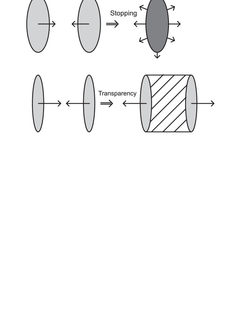
Figure 12: Nucleus-nucleus collisions at $\sqrt{s}\ll 100$ GeV (stopping) and at $\sqrt{s}\simeq 100$ GeV or larger (transparency).

There are two basic scenarios for the space-time evolution of the fireball in relativistic heavy-ion collisions [109] as shown in Fig. 12. For collision energies $\sqrt{s}\ll 100$ GeV (AGS, SPS), the nuclei are stopped in the collision to a large extent and a dense and hot expanding fireball with a finite baryon density (finite chemical potential) is formed, which might be in the QGP phase initially if the critical temperature $T_{c}$ of about 150 - 170 MeV is exceeded. The expansion leads to a temperature drop until $T_{c}$ is reached, at which hadronization sets in. After a potential mixed phase and hadronic phase, the interactions in the fireball will finally freeze out allowing the hadrons to propagate freely. In the second scenario, expected to be valid for $\sqrt{s}\simeq 100$ GeV or larger (RHIC, LHC), there is not enough time for the highly Lorentz contracted nuclei to be stopped in the nucleus-nucleus collision. Rather they propagate through each other approximately transparently. However, the vacuum between the receding nuclei will be highly excited from the initial hard parton collisions and will decay violently into a baryon-free (zero chemical potential) parton gas by secondary parton collisions or, in a non-perturbative picture, by string decay. The secondary collisions will drive the parton gas to thermal equilibrium, corresponding to the QGP stage. The system is mainly expanding in beam direction in a boost-invariant way (Bjorken scenario) [110, 111], accompanied by a cooling of the fireball. The various stages, mixed phase, hadronic phase, and freeze-out, follow as in the first scenario. The space-time diagram of the second scenario, showing the various stages, is sketched in Fig. 13. The $z$-axis agrees with the beam direction. At $t=0$, the maximum overlap of the nuclei takes place. The produced particles in this diagram lie above the light-cone due to causality. The hyperbolas denote curves of constant proper time $\tau=\sqrt{t^{2}-z^{2}}$, on which the same physics, e.g. energy density and temperature, occurs, according to the boost-invariant Bjorken scenario [110].

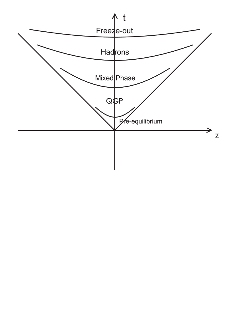
Figure 13: Space-time diagram of a ultrarelativistic heavy-ion collision in the Bjorken scenario.

In order to speak of the QGP as a thermal system, we need a large volume and particle number, and a sufficiently long life-time of the equilibrated system. Rough estimates give a sufficiently large volume of the order of 1000 fm³ at RHIC or LHC, a large parton number up to about a several thousand, and a sufficiently long life-time of the parton gas of 5 - 10 fm/c before hadronization sets in. For the formation time of the QGP a typical value of the order of 0.5 - 1 fm/c has been accepted [112]. However, doubts have been raised, whether the parton gas in a heavy-ion collision will reach a thermalized stage at all, at least by elastic scatterings as assumed usually [113]. Moreover, the realization of a chemical equilibrium between gluons and light quarks appears to be questionable at RHIC and LHC [114, 115].

In order to describe the dynamical evolution of a many-particle system in non-equilibrium or equilibrium, transport models are adopted. Starting from the Boltzmann equation [116], describing the transport of different interacting hadron species semi-classically [117], particle production, e.g. photon production, in heavy-ion collisions up to collision energies of about 1 A$\cdot$GeV can be treated successfully [118]. Transport models have also been used to describe the photon spectrum in relativistic heavy-ion collisions [119]. However, in these approaches only a hadron gas but not a QGP phase has been considered, which requires the transport theoretical description of a parton gas. Although such microscopic models for the parton-gas dynamics based on perturbative QCD exist [120, 121], they have not been applied to photon production from the QGP so far. Hence, no transport theoretical predictions of photon spectra in relativistic heavy-ion collisions taking into account a QGP phase are available.

To illustrate the hydrodynamical calculation of the photon spectrum, we will consider in detail a simple hydrodynamical model in the following. This model is certainly oversimplified as it neglects the transverse expansion of the fireball and is based on an unrealistic EOS, which leads to a strong first order phase transition and a long-lived mixed phase in contradiction to lattice results [14]. More realistic hydrodynamical descriptions including transverse flow and an improved EOS will be discussed subsequently.

Assuming a local thermal and chemical equilibrium hydrodynamical equations can be derived from the Boltzmann equation [116]. The relativistic hydrodynamical equations follow from the conservation of the baryon number, energy, and momentum. If we assume an ideal fluid, i.e. neglect dissipative effects, the energy-momentum tensor is given by

$$T^{\mu\nu}=(\epsilon+P)\>u^{\mu}\,u^{\nu}-P\>g^{\mu\nu},$$ (14)

where $\epsilon$ is the energy density, $P$ the pressure, $u^{\mu}=\gamma(1,{\bf v})=\partial x^{\mu}/\partial\tau$ ($\gamma=1/\sqrt{1-{\bf v}^{2}}$) the (local) 4-velocity of the fluid, and $g^{\mu\nu}$ the Minkowski metric. From the conservation of the energy-momentum tensor, $\partial_{\mu}T^{\mu\nu}=0$, multiplied by $u^{\nu}$, the relativistic Euler equation follows

$$u^{\mu}\>\partial_{\mu}\epsilon+(\epsilon+P)\partial_{\mu}u^{\mu}=0.$$ (15)

Assuming for simplicity only a longitudinal boost-invariant expansion, i.e. $u^{\mu}=x^{\mu}/\tau$, (Bjorken scenario [110]), as it might be the case approximately at RHIC and LHC energies, the Euler equation can be written as

$$\frac{d\epsilon}{d\tau}+\frac{\epsilon+P}{\tau}=0.$$ (16)

For an ideal ultrarelativistic gas, such as the non-interacting QGP, $\epsilon=3P$ holds and the evolution of the energy density, depending only on time, can be determined easily: $\epsilon=\epsilon_{0}\>(\tau_{0}/\tau)^{4/3}$. Furthermore, one obtains $T=T_{0}\>(\tau_{0}/\tau)^{1/3}$. Here $\tau_{0}$, $\epsilon_{0}$, and $T_{0}$ are the initial time, energy density, and temperature, respectively. They are determined by the time at which the local equilibrium has been achieved.

The results of a hydrodynamical model depend strongly on the choice of the initial conditions. Therefore a reliable determination of the initial conditions is crucial. The initial conditions can be taken in principle from transport calculations describing the approach to equilibrium, such as the parton cascade model (PCM) [120] or HIJING [121], which treat the entire evolution of the parton gas from the first contact of the cold nuclei to hadronization. However, there are no unambiguous criteria for determining the completion of the equilibration process in these transport models. Another possibility for fixing the initial conditions comes from relating observables to the initial conditions. For example, the initial temperature can be related to the particle multiplicity $dN/dy$, assuming an ideal parton gas with an isentropic expansion [20]

$$T_{0}^{3}=\frac{c}{4a}\>\frac{1}{V_{0}}\>\frac{dN}{dy}.$$ (17)

Here $V_{0}=\pi R_{A}^{2}\tau_{0}$ is the initial volume with the nucleus radius $R_{A}\simeq 1.3\>A^{1/3}$ fm, For the initial time $\tau_{0}$, one usually assumes values of the order of 1 fm/c. Furthermore, $c=2\pi^{4}/(45\zeta(3))\simeq 3.6$ and $a=8\pi^{2}/45+7\pi^{2}N_{F}/60$ with $N_{F}$ light quark flavors.

Another relation between the initial temperature and the initial time, which is used frequently, is based on an argument using the uncertainty principle [122]. The formation time $\tau$ of a particle with an average energy $\langle E\rangle$ is given by $\tau\langle E\rangle\simeq 1$. The average energy of a thermal parton is about $3T$. Hence, we find $\tau_{0}\simeq 1/(3T_{0})$. However, the formation time of a particle, i.e. the time required to reach its mass shell, is not necessarily identical to the thermalization time [122]. Consequently, the determination of the initial conditions is far from being trivial. However, if data for hadron production are available, such as at SPS, they can be used to determine or at least constrain the initial conditions for a hydrodynamical calculation of the photon spectra [123].

Another essential ingredient for a hydrodynamical model is the EOS. Since we want to describe a fireball undergoing a phase transition, we need an EOS for the QGP as well as for the HHG. The QGP EOS has been determined in lattice QCD [124, 6], which shows a clear deviation from an ideal QGP at temperatures accessible in heavy-ion collisions. In most hydrodynamical calculations, however, a simple bag model EOS has been used for the QGP [125]. For a vanishing chemical potential, the pressure and energy density in this model are given by

$$P_{q} = g_{q}\>\frac{\pi^{2}}{90}T^{4}-B,$$

$$\epsilon_{q} = g_{q}\>\frac{\pi^{2}}{30}T^{4}+B,$$ (18)

where the effective number of degrees of freedom is

$$g_{q}=2\>(N_{C}^{2}-1)+\frac{7}{8}\>4\>N_{C}\>N_{F}$$ (19)

with the number of colors $N_{C}=3$. For two active quark flavors ($N_{F}=2$) one gets $g_{q}=37$ and for three ($N_{F}=3$) $g_{q}=47.5$, respectively. The bag constant $B$ is related to the critical temperature (see below) and typically of the order $B^{1/4}=200$ MeV. The EOS is given by $\epsilon_{q}=3P_{q}+4B$.

For the HHG EOS usually an ideal hadron gas is adopted. However, the number of hadron species included varies. Typically, all hadrons up to masses of 2 or 2.5 GeV are taken. For illustration we will restrict ourselves to a massless pion gas [126]. Then the pressure and energy density are given by

$$P_{h} = g_{h}\>\frac{\pi^{2}}{90}T^{4},$$

$$\epsilon_{h} = g_{h}\>\frac{\pi^{2}}{30}T^{4}$$ (20)

with $g_{h}=3$ and $\epsilon_{h}=3P_{h}$. In fact, comparing the photon spectrum at SPS energies, obtained by using this simple EOS, with results from using more realistic EOS, e.g. [127], one finds that $g_{h}=3$ should be replaced by $g_{h}=8$ [51].

The two EOS are matched together by the Gibbs criteria: $T_{c}^{q}=T_{c}^{h}=T_{c}$ and $P_{c}^{q}=P_{c}^{h}=P_{c}$. Together with Eqs. (18) and (20) a relation between the bag constant and the critical temperature follows

$$T_{c}^{4}=\frac{90B}{(g_{q}-g_{h})\pi^{2}}.$$ (21)

For instance, a bag constant of $B^{1/4}=200$ MeV implies $T_{c}=144$ MeV for $g_{q}=37$ and $g_{h}=3$. Now in addition to the initial conditions, $\tau_{0}$ and $T_{0}$, there are two more parameters, namely the critical temperature $T_{c}$ and the freeze-out temperature $T_{f}$, where the hydrodynamical evolution ceases. The critical temperature, predicted by lattice QCD, is in the range $170\pm 20$ GeV [6], and the freeze-out temperature should be between 100 and 160 MeV [128].

Figure 14: Energy density and temperature evolution for $g_{q}=37$, $g_{h}=3$, $\tau_{0}=1$ fm, $T_{0}=250$ MeV, $T_{c}=170$ MeV, and $T_{f}=150$ MeV [126].

The construction above implies the existence of a mixed phase corresponding to a first-order phase transition (see Fig. 14). Although lattice QCD favors a continuous phase transition instead of a first-order transition [14], lattice calculations show also a rapid change in the energy density similar as in the bag and pion gas model due to a large increase in the number of degrees of freedom going from the HHG to the QGP. The life-times of the different phases in our simple model are given by [126]

$$\Delta\tau_{q} = \tau_{0}\>\left[\left(\frac{T_{0}}{T_{c}}\right)^{3}-1\right],$$

$$\Delta\tau_{c} = \tau_{0}\>\left(\frac{T_{0}}{T_{c}}\right)^{3}\>\left[\frac{g_{q}}{g_{h}}-1\right],$$

$$\Delta\tau_{h} = \tau_{0}\>\left(\frac{T_{0}}{T_{c}}\right)^{3}\>\left[\left(\frac{T_{c}}{T_{f}}\right)^{3}-1\right],$$ (22)

where $\Delta\tau_{c}$ denotes the life-time of the mixed phase, during which the temperature $T=T_{c}$ stays constant. The life-times of the different phases as a function of the initial and the critical temperature are shown in Fig. 15 and Fig. 16. The simple EOS of a massless pion gas leads to a strong first-order transition and hence to a very long-living mixed phase. Hence, it is important to use a realistic EOS for the HHG. In particular, in the no-phase-transition scenario, to which the phase-transition scenario has to be compared for predicting signatures, a realistic EOS is essential. For example, the initial temperature in the massless pion gas has to be chosen unrealistically high ($T_{0}=578$ MeV), if the initial temperature of the QGP is $T_{0}=250$ MeV and identical values for the initial time and the entropy are assumed in both scenarios [129].

Figure 15: Life-times of the QGP (dashed line), the mixed phase (dash-dotted line), and the HHG (dotted line) as a function of $T_{0}$ [126].

Figure 16: Life-times of the QGP (dashed line), the mixed phase (dash-dotted line), and the HHG (dotted line) as a function of $T_{c}$ [126].

The hydrodynamical model presented above for illustration is certainly oversimplified. A transverse expansion cannot be neglected, in particular in the later stages of the fireball, changing the photon spectra significantly at RHIC and LHC (see below). There are different hydrodynamical models for relativistic heavy-ion collisions on the market, which describe the expansion of the fireball in 2 or 3 space dimensions [130, 131]. Of course, the hydrodynamical equations can only be solved by rather elaborate numerical techniques in this case. Also it might not be justified to restrict to an ideal fluid, but dissipation might be important. For example, perturbative estimates of the viscosity of the QGP yielded a large value [132, 133]. Hence, the Euler equation should be replaced by the Navier-Stokes or even higher order dissipative equations. However, dissipative effects render the numerical treatment much more difficult and introduce new parameters such as viscosity [130]. After all, first attempts in this direction have been undertaken already [134].

Under the simplifying assumption of an ideal fluid, the hydrodynamical equations can be solved numerically using the respective EOS for each of the two phases and the initial conditions, such as initial time and temperature, as input. The final results depend strongly on the input parameters as well as on other details of the model, as in the simple 1-dimensional case. Also it is important to adopt a realistic EOS, in particular for the hadron gas, as discussed above.

Finally, the deviation from a chemically equilibrated QGP, which is expected to be important at RHIC and LHC [114, 115], should be taken into account. It is expected that the parton gas at RHIC and LHC energies will be thermalized rapidly on a time scale of 0.5 to 1 fm/c [120, 121]. However, a chemical equilibration of the plasma might require much more time if it is realized at all [114, 115]. This means that the parton abundances are less than their equilibrium value. In order to describe the deviation from chemical equilibrium, a time-dependent gluon or quark suppression factor $\lambda_{g,q}(\tau)$, sometimes called fugacity, is introduced. Then the non-equilibrium distribution functions read $f_{g}(E,\tau)=\lambda_{g}(\tau)\,n_{B}(E)$ and $f_{q}(E,\tau)=\lambda_{q}(\tau)\,n_{F}(E)$, respectively. For example, the energy density at zero baryon density is now given by $\epsilon=(\lambda_{g}a_{g}+\lambda_{q}a_{q})\,T^{4}$, where $a_{g}=8\pi^{2}/15$ and $a_{q}=7\pi^{2}N_{F}/20$. This expression can be used in Bjorken’s hydrodynamic equation Eq. (16), which yields $[\lambda_{g}+(a_{q}/a_{g})\lambda_{q}]^{3/4}\>T^{3}\tau={\rm constant}$ [114].

The parton phase space will be populated by inelastic parton reactions producing quarks and gluons. To lowest order those are: $gg\rightarrow q\bar{q}$ and $gg\rightarrow ggg$. The time dependence of the fugacities can now be determined from rate equations, which contain the cross sections for theses processes [114]. As a subtle point, screening masses (Debye screening, thermal quark mass) have to be used to cut off IR singularities in these cross sections. These screening masses also depend on the fugacities, as screening is less efficient in a dilute system [114]. Solving the rate equations together with Bjorken’s hydrodynamic equation, the time-dependence of the fugacities and the temperature is obtained. The initial values for the temperature and the fugacities can be taken from PCM [120] or HIJING [121] at the moment at which thermalization is completed, i.e., as soon as there are approximately exponential and locally isotropic momentum distributions [114]. Using HIJING initial conditions, the initial fugacities are far from their equilibrium value, $\lambda_{g,q}^{\rm eq}=1$, in particular for the quark component, $\lambda_{q}^{0}\ll 1$. Larger initial fugacities follow from the PCM. Anyway, due to the larger cross sections for gluon production, one expects much more gluons than quarks in the early stages of the fireball, which is called the “hot glue” scenario [135]. The fugacities increase with time but might never reach their equilibrium value before hadronization sets in, in particular at RHIC [114]. At the same time the temperature of the fireball drops even more rapidly than in equilibrium because the production of partons consumes energy.

The above picture of chemical equilibration can also be incorporated in more realistic hydrodynamical models containing also a transverse expansion [136]. It has been shown that the system evolves initially to chemical equilibrium but will be driven away from it at a later stage, in which the transverse flow becomes important.

For predicting photon spectra from a chemically non-equilibrated QGP, it is not only necessary to modify the hydrodynamics, but also the photon production rates change. Starting from Eq. (2), the equilibrium distribution functions have now to be replaced by $f_{g,q}$, containing the fugacities. Also the fugacities have to be considered, for example, in the thermal quark mass in Eq. (4), $m_{q}^{2}=(\lambda_{g}+\lambda_{q}/2)\,g^{2}T^{2}/6$ [114], serving as an IR cutoff. Modified rates for photon production from Compton scattering, annihilation, and bremsstrahlung, obtained in this way, have been used to predict photon spectra for RHIC and LHC [46, 47, 52, 53, 137], which we will discuss in Section 4. A more sophisticated way is to calculate the non-equilibrium rates by generalizing the HTL method to chemical non-equilibrium [48, 138]. Baier et al. [48] have calculated the 1-loop HTL photon production rate in this way and found results similar to the ones of the simplified approach of Ref.[47].

Recently, Wang and Boyanovsky [139, 140] found a significant enhancement of the photon production for $p_{T}>1.0$ - 1.5 GeV due to the finite life-time of the QGP. Considering this non-equilibrium effect within the real time formalism, they obtained a power law spectrum for the photons from off-shell quark bremsstrahlung, $q\rightarrow q\gamma$.

2.2.2 Photon Spectra

As emphasized already a few times, photon spectra follow from convoluting the photon production rates with the space-time evolution of the heavy-ion collision, for which usually hydrodynamical models are employed,

$$E\,\frac{dN}{d^{3}p}=\int d^{4}x\>E\,\frac{dN}{d^{4}x\,d^{3}p}.$$ (23)

Here, the rate on the right-hand-side depends on the temperature, which depends in turn on the space-time coordinate in accordance with the assumption of a local equilibrium.

For illustration, but also because it is widely used, we will discuss the calculation of the spectra using simple Bjorken hydrodynamics, following Ref.[126]. In this model the fireball is a longitudinally expanding cylinder. Hence, we can write

$$\int d^{4}x=\pi\,R_{a}^{2}\;\int dt\;dz,$$ (24)

where $R_{A}\simeq 1.3\>A^{1/3}$ fm and $z$ is the beam axis. It is convenient to make a coordinate transformation to proper time $\tau$ and rapidity $y^{\prime}$ of the emitting fluid cell, i.e. $t=\tau\>\sinh y^{\prime}$ and $z=\tau\>\cosh y^{\prime}$, yielding

$$\int dt\;dz=\int_{\tau_{0}}^{\tau_{f}}d\tau\,\tau\;\int_{-y_{\rm nucl}}^{+y_{\rm nucl}}dy^{\prime},$$ (25)

where $\tau_{0}$ and $\tau_{f}$ are the initial and freeze-out times and $y_{\rm nucl}=\mathrm{arcosh}[\sqrt{s}/(2A\cdot{\rm GeV})]$ [131] is the center-of-mass projectile rapidity. For SPS ($\sqrt{s}=17A\cdot{\rm GeV}$) one finds $y_{\rm nucl}=2.8$, for RHIC ($\sqrt{s}=200A\cdot{\rm GeV}$) $y_{\rm nucl}=5.3$, and for LHC ($\sqrt{s}=5500A\cdot{\rm GeV}$) $y_{\rm nucl}=8.6$. Using $E/d^{3}p=1/(d^{2}p_{T}dy)$ with the transverse momentum $p_{T}$ and the rapidity $y$ of the photon, one arrives at

$$\frac{dN}{d^{2}p_{\perp}\,dy}=\pi\,R_{A}^{2}\;\int_{\tau_{0}}^{\tau_{f}}d\tau\,\tau\;\int_{-y_{\rm nucl}}^{+y_{\rm nucl}}dy^{\prime}\,E\,\frac{dN}{d^{4}x\,d^{3}p}.$$ (26)

The thermal photon spectrum is defined in the center-of-mass system and the photon rate on the right-hand-side in the local rest frame of the emitting fluid cell, where the photon energy is given by $E=p_{T}\>\cosh(y^{\prime}-y)$.

During the mixed phase the photon production rate is given as

$$E\,\frac{dN}{d^{4}x\,d^{3}p}=\lambda(\tau)\>\left(E\,\frac{dN}{d^{4}x\,d^{3}p}\,\right)_{QGP}+[1-\lambda(\tau)]\>\left(E,\frac{dN}{d^{4}x\,d^{3}p}\,\right)_{HHG},$$ (27)

where $\lambda(\tau)=V_{\rm QGP}(\tau)/V_{\rm tot}(\tau)$ is the QGP volume fraction.

Figure 17: Photon spectra at an initial temperature $T_{0}=200$ MeV (above) and 300 MeV (below). The dashed line corresponds to the spectrum from the QGP, the dotted one to the spectrum from the HHG, and the solid one to the sum of both [126].

Eq. (26) together with the estimates for the rates from the QGP and the HHG allows a systematic investigation of the photon spectrum, depending on the mass number $A$, the projectile rapidity $y_{\rm nucl}$, the thermalization time $\tau_{0}$, the initial temperature $T_{0}$, the critical temperature $T_{c}$, and the freeze-out temperature $T_{f}$. In the following all spectra are calculated for photons at mid-rapidity $y=0$. The following results have been obtained [126]: The photon spectrum is proportional to $R_{A}^{2}$ (see Eq. (26)), i.e. $dN/(d^{2}p_{T}dy)\sim A^{2/3}$. The dependence of the spectra on the limits of the rapidity integration $y_{\rm nucl}$ is very weak since photons from a fluid cell with $y^{\prime}$ far away from zero do not contribute to mid-rapidity photons because they must have a large energy in the local rest frame of the fluid cell and are therefore exponentially suppressed in the rate. However, the collision energy, from which the projectile rapidity follows, determines the initial time and temperature, which have an important influence on the spectrum. In fact, one can show that $dN/(d^{2}p_{T}dy)\sim\tau_{0}^{2}$ [126]. At higher collision energies, smaller thermalization times are expected [114]. At the same time the initial temperature is increased, which is the dominating factor. For example, an increase of the initial temperature from $T_{0}=200$ MeV to 300 MeV increases the thermal photon yield by more than a magnitude for a fixed initial time [126]. In particular, high $p_{T}$ photons are enhanced, i.e., the spectrum gets flatter corresponding to a higher temperature. The reason for this enhancement of the yield is the longer life-time of the fireball and the larger rates at higher $T_{0}$ (see Fig. 15). The dependence of the spectrum on $T_{0}$ is exemplified in Fig. 17. As can be seen from Fig. 16, an increase of $T_{c}$ will result in a decrease of the life-times of the QGP and the mixed phase and an increase of the HHG life-time. Depending on the rates from the different phases, this affects the spectrum. Using the rates discussed above one observes an increase of the spectrum by about a factor of 5 going from $T_{c}=160$ MeV to $T_{c}=200$ MeV (see Fig. 18), due to a higher mean temperature in the latter case. A lower value of $T_{f}$ implies a longer life-time of the HHG. However, since the rates are small at low temperatures, a change of the freeze-out temperature is negligible in this simple model. However, taking into account a transverse expansion, this statement will be changed.

Figure 18: Photon spectra at a critical temperature $T_{c}=160$ MeV (above) and 200 MeV (below), where the same notation as in Fig. 17 is used [126].

The role of a finite chemical potential on the photon spectra will be discussed in connection with the comparison of the theoretical spectra with SPS data from WA80 and WA98 in Section 4. The modifications of the spectra due to a chemical non-equilibrium will be considered in the predictions of spectra for RHIC and LHC (Section 4).

So far, different aspects of the hydrodynamical calculation of photon spectra in relativistic nucleus-nucleus reactions have been investigated. The various results for SPS, RHIC and LHC, using different hydrodynamical models and rates, will be reviewed in Section 4, where also the prompt photon spectrum will be considered. However, a systematic and comprehensive hydrodynamical calculation of photon spectra together with dilepton and hadronic spectra from SPS to LHC energies, considering the most recent rates, a realistic EOS, a reasonable fixing procedure for the initial conditions, transverse expansion, and chemical non-equilibrium, is missing. Hence, besides the problems with the rates, the ambiguities in the description of the fireball evolution are another main source for uncertainties in the theoretical prediction of photon spectra in relativistic heavy-ion collisions [141]. After all, simple hydrodynamical models, e.g. with a simplified EOS and without transverse expansion, can be useful to study systematically certain aspects such as the dependence on different parameters (initial time and temperature, critical temperature, etc.) or the relative importance of different contributions to the spectrum [126, 51].

3 Experiments

The detection of electromagnetic radiation may involve very different technologies, just because for the possible energies or wavelengths very different physics is relevant, ranging from atomic and molecular processes at low energy to particle physics concepts at high energy, the latter being important for the subject of this report, where we deal with photon energies in the GeV range. In this regime one concentrates on measuring individual quanta, i.e. photons, and their four-momenta. Huge detectors weighing up to several hundred tons are employed to perform this measurement of individual photons. For essentially all of these detectors, the photons have to be converted into charged particles which eventually will be measured.

3.1 Experimental Methods

In the following Section the experimental foundations of direct photon measurements are discussed. For this purpose we present different methods for inclusive photon detection and discuss in the following the further requirements for the identification of the direct fraction of the measured photons.

3.1.1 Photon Detection

High energy photon detectors can be divided into two main categories depending on the detection principle:

1. electromagnetic calorimeters, which attempt to measure the total energy which has been deposited in a given amount of material by an electromagnetic cascade following the first conversion and

2. conversion detectors, which combine the photon conversion into e⁺e^- with the subsequent momentum measurement of the charged leptons by tracking.

In its ideal forms these two different types of detectors have complementary merits. On the one hand, the energy measurement in a calorimeter is affected by statistical number fluctuations in the electromagnetic shower which become less and less important for photons of higher energy, while the momentum determination of the conversion products in a tracking system has to deal with the measurement of smaller deflections of tracks with increasing e⁺,e^--momenta. Calorimeters are therefore generically better suited for very high energy photons. In addition, converters are required to be relatively thin to allow for precise momentum measurement from just the two conversion products so that the detection probability (which includes the conversion probability) is relatively low, while calorimeters usually have detection probabilities of essentially $100\%$. Calorimeters are also intrinsically fast which allows to use them for triggering purposes.

On the other hand, the momentum measurement from tracking devices yield pointing capabilities far superior to calorimeters which in their basic configurations have almost none — this can help considerably to reduce potential backgrounds of particles not originating from the reaction studied, as e.g. cosmic rays or beam halo. The conversion measurement should also suffer less from misidentification of other particles, which might still yield signals in a calorimeter. This is most important for relatively small photon energies. Furthermore, calorimeters have inherent limits with regard to the separation of two particles with small opening angles because of the finite lateral dimensions of showers in the detector material, while even for very small angular separations of the photons the e⁺e^--pairs may have very well separated tracks allowing them to be individually detected in a conversion/tracking device. This may be of importance for more sophisticated measurements like two-photon-correlations, but will also have an impact on detection capabilities in a high multiplicity environment or for extremely high momenta, where hadron decay photon pairs start to merge in a calorimeter.

Calorimeters have been most widely used for the detection of high energy photons because of their advantages sketched above. One should, however, keep in mind that the conversion method may be advantageous in special situations, and that for very precise measurements the combination of both methods may be considered, as they should be affected by very different sources of systematic error. Electromagnetic calorimeters are constructed as either homogeneous or as sampling calorimeters. Sampling calorimeters are built using a high-$Z$ material (e.g. $Pb$) as absorber and an active material (very frequently light generating like plastic scintillator) in consecutive layers. Homogeneous calorimeters use one material which serves as both absorbing and active material. They can in principle achieve much better detector performance than sampling calorimeters because of the additional sampling fluctuations in the latter.

Examples of high energy photon detectors used include

• lead-scintillator-sandwich calorimeters [142, 143, 144, 145, 146, 147, 148, 149, 150, 151],

• lead glass calorimeters which measure the Cherenkov light emitted by shower particles via photomultiplier tubes [152, 153, 154, 155, 156, 157],

• calorimeters out of scintillating crystals like $NaI$ [158, 159, 160] or $BGO$ [161] readout via either phototubes or photodiodes,

• liquid-argon calorimeters which are sampling detectors measuring the specific ionization of charged shower particles in wire chambers filled with liquid argon [162, 163, 164, 165, 166, 167],

• lead-proportional tube sampling calorimeters [168] and

• converters combined with magnetic electron-positron-pair spectrometers [169, 170, 171, 172].

Homogeneous calorimeters made of scintillating crystals are generally superior in energy resolution due to their high light output. Sampling calorimeters suffer from additional sampling fluctuations but are much less expensive, especially if detectors of large thickness are required to allow containment of very high energy photon showers. Of course, the higher the photon energy, the less important is the intrinsic energy resolution of a calorimeter.

Another important figure of merit is the suppression of hadrons. Most calorimeter materials have much longer hadronic interaction length compared to their radiation length. Hadrons are very unlikely to deposit a considerable fraction of their energy and are effectively suppressed at high energies. A similar effect helps in suppressing a large fraction of muons. Further hadron suppression can be achieved by exploiting the differences in shape of showers induced by hadrons or photons, with electromagnetic showers being usually much better contained. A fine lateral segmentation allows to discriminate showers from their lateral width, which is larger for hadronic showers. Longitudinal segmentation can sample the depth profile - hadronic showers penetrate deeper into the detector.

A combination of sufficient longitudinal and lateral segmentation can even provide pointing capabilities which help to suppress background particles which do not originate from the interaction vertex.

For further suppression of charged particles additional tracking detectors can be used. These will also help to reduce the contamination by the usually small fraction of electrons and positrons produced, i.e. charged particles generating electromagnetic showers in calorimeters. The detectors may either be specialized charged particle veto detectors, like multiwire proportional chambers [142, 143, 144, 145, 146, 155] or streamer tube detectors [156, 157], providing the point of impact of charged particles just in front of the calorimeter or full magnetic spectrometers [147, 148, 149, 150, 151, 166, 167].

For direct photon measurements other requirements, like e.g. knowledge of the detector response or particle discrimination capabilities, become more and more important. Thus the detector choice may well depend on the particular measurement “strategy” that is used.

3.1.2 Direct Photon Identification

In particle physics experiments one usually tries to achieve an individual identification of direct photons. The environment is such that photons from meson decays (mostly from pions) will be both detected with high probability in a certain energy range. Photons detected as single, i.e. no appropriate other photon is measured which would combine with the candidate to a known hadron, may be treated as direct photons and only small corrections for detection efficiency or finite geometrical acceptance have to be applied. Random coincidences of two particles which fake a photon combination originating from a hadron decay are rare and can be neglected. In collider experiments (see e.g. [150, 151, 166, 167]) one usually requires photons to be isolated, i.e. not accompanied by any other cluster in the calorimeter. In addition to the suppression of multi-photon background from hadron decays, this also suppresses direct photons produced by Bremsstrahlung processes of hard quarks, which would be observed close to the jet fragmentation products. For very high photon energies the discrimination of single photons against neutral mesons, esp. pions, decaying into two photons with a small opening angle becomes extremely important. For these cases the two photon showers can not be separated. Two different methods have been used to statistically estimate the contamination [150, 151, 166, 167]:

1. The shower shape is measured in a dedicated detector and compared with simulated shower shapes from direct photons and from the expected background.

2. The higher conversion probability in the first layers of the detector for two collinear photons compared to a single photon is used to estimate the background from the longitudinal distribution of the shower.

Uncertainties of the direct photon measurement in particle physics experiments include:

1. Background from beam halo (muons), beam-gas events or other no-target contributions,

2. multi-event pile-up,

3. trigger efficiency,

4. misidentified charged and neutral hadrons (important in calorimeters at lower energies),

5. contamination from merged neutral pions (important in calorimeters at higher energies),

6. single photons from hadron decays (important for small detector acceptance and/or asymmetric decays),

7. energy scale uncertainty,

8. conversion probability in conversion measurements,

9. loss of photons from conversion and

10. uncertainty of luminosity, target thickness etc. (overall scale uncertainty) .

Heavy-ion experiments have the additional difficulty of dealing with high multiplicities already at relatively low energies. It is therefore not possible to identify individual direct photons. One has to resort to a statistical identification of direct photons. For any given photon there is a high probability that another random photon is detected which would combine well with the first to a potential hadron decay photon pair. The only possible strategy is therefore to measure all inclusive photons regardless of their origin and to subtract the photons originating from hadron decays (see e.g. [157]). For most situations, where the fraction of direct photons compared to all photons is relatively small, this implies that the direct photon result is obtained by subtracting two large numbers. Therefore such analyses are even more sensitive to systematic errors. To the sources of systematic uncertainty cited above have to be added:

1. effects of a multiplicity dependent detector response.

This includes e.g. the influence of randomly overlapping showers in a calorimeter.

Other crucial sources of systematic error in this situation are related to the determination of the decay photons from hadrons, most importantly neutral pions and $\eta$ mesons. The preferred option is of course to measure the production of neutral mesons simultaneously in the same data set as the inclusive photons. Such a measurement is usually performed by a two-photon invariant mass analysis [157]. Even if the two-photon decay mode is not the only decay producing background photons (there is e.g. the Dalitz decay $\pi^{0}\rightarrow\mathrm{e^{+}e^{-}}\gamma$), the known branching ratios allow to calculate all relevant decay contributions. In this case the following systematic uncertainties on the relative amount of meson decay photons may contribute:

1. Uncertainty of the subtraction of combinatorial background,

2. effects of multiplicity dependent detector response on the meson reconstruction (different from item 11),

3. geometrical acceptance,

4. loss of mesons from photon conversion,

5. loss of mesons from merging photon showers and

6. those effects from the energy scale uncertainty, from beam-gas events or other no-target contributions which differ from the effects on inclusive photons.

Any uncertainty on the overall normalization of the cross sections (like those mentioned under item 10) does not enter here, if the meson spectra are determined from the same data sample. Those hadrons decaying into photons, which are not measured, have to be estimated from other sources. This is usually the case for heavier mesons (e.g. $\omega$, $\eta^{\prime}$), which contribute only a very small fraction to the total number of decay photons. In conversion measurements, however, already the detection of neutral pions is very difficult and can very often not be done, because the single photon detection probability is low. This may introduce a very large systematic uncertainty of the decay background to be subtracted and has to be treated with great care.

3.2 Experimental Results

3.2.1 $pp$ and $pA$ Experiments

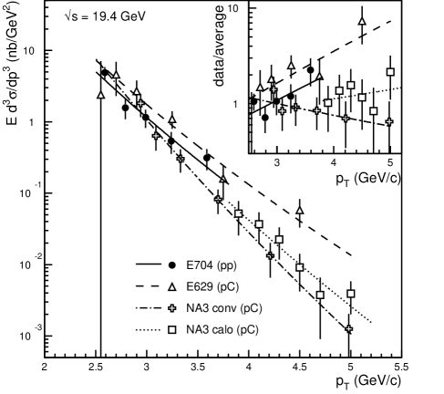
Figure 19: Direct photon cross section per nucleon for $p$-induced reactions at $\sqrt{s}=19.4\,\mathrm{GeV}$. Data are from experiments E704 [155], E629 [164] and NA3 [169]. The inset shows the ratios of experimental data to a simultaneous fit to all data sets.

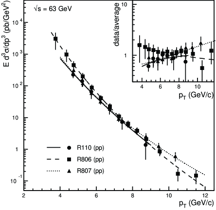
Figure 20: Direct photon cross section for $pp$ reactions at $\sqrt{s}=63\,\mathrm{GeV}$. Data are from experiments R110 [154], R806 [162] and R807 (AFS) [159]. The inset shows the ratios of experimental data to a simultaneous fit to all data sets.

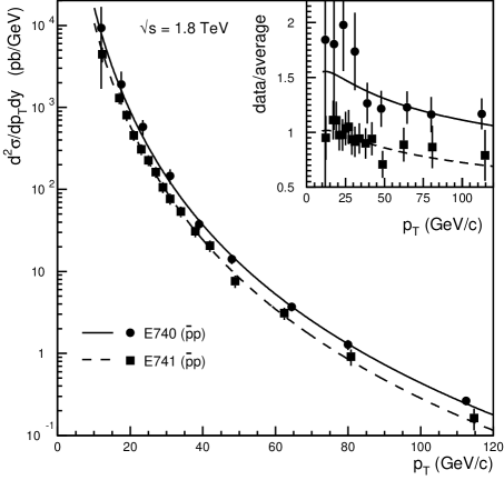
Figure 21: Direct photon cross section for ${\bar{p}p}$ reactions at $\sqrt{s}=1.8\,\mathrm{TeV}$. Data are from experiments E740 (D0) [167] and E741 (CDF) [150]. The inset shows the ratios of experimental data to a simultaneous fit to all data sets.

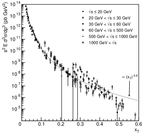
Figure 22: Direct photon cross section scaled with $s^{2}$ for $pp$ and $\bar{p}p$ reactions at different energies. The dashed line shows a fit of a power law according to Eq. (29) to all data sets.

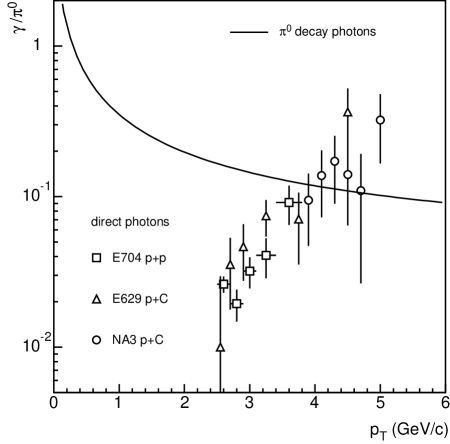
Figure 23: $\gamma/\pi^{0}$ ratio as a function of $p_{T}$ for $\sqrt{s}=19.4\,\mathrm{GeV}$. The open symbols show the values for direct photons extracted in $pp$ and $pC$ experiments. The solid line shows an estimate of the ratio for decay photons from $\pi^{0}$.

A great wealth of experimental results from $pp$ and $pA$ experiments is available. For a compilation of these results see e.g. [92]. The beam energies range from $\sqrt{s}=19.4\,\mathrm{GeV}$ to $\sqrt{s}=1.8\,\mathrm{TeV}$. The lowest energy data (up to $\sqrt{s}=30.6\,\mathrm{GeV}$) have been measured in fixed-target experiments at CERN [142, 144, 145, 146, 143, 152, 168, 169, 170], and Fermilab [155, 164, 165] while the data at higher energies are from collider experiments at ISR [153, 154, 158, 159, 160, 162, 163], SPS [147, 148, 149] and the Tevatron [150, 151, 166, 167].

We will only discuss some of the experimental results in different energy regimes as examples for the experimental achievements in this field. We have chosen energies for which different data sets exist which may be compared. The lowest beam energy at which direct photon data are available is $\sqrt{s}=19.4\,\mathrm{GeV}$. At this energy cross sections for direct photons are measured in $pp$ reactions by the Fermilab experiment E704 [155], and by two experiments in $p$+$C$ reactions, E629 [164] at Fermilab and NA3 [169] at CERN. These data are shown in Fig. 19 together with fits of the phenomenological function [173]:

$$E\frac{d^{3}\sigma}{dp^{3}}=A\cdot\left(\frac{p_{0}}{p_{T}+p_{0}}\right)^{n}.$$ (28)

The NA3 experiment has performed measurements using two independent techniques, i.e. measurements using a calorimeter (label “calo”) and conversion measurements (label “conv”). There are considerable discrepancies between the different data sets — these can be judged more easily from the inset, where the different data sets are normalized to a common fit to all data points. The results from E629 are considerably above the other data sets, especially the measurement at the highest $p_{T}$, which is about a factor of 10 higher. All data sets show different slopes, and the overall discrepancies, even ignoring the high $p_{T}$ point of E629, are of the order of a factor of 3 which is mostly covered by the experimental error bars.

As the discrepancies appear to be smallest at low $p_{T}$ and increase with higher $p_{T}$ it is likely that energy scale uncertainties play a role here. Still the variations even between the two data sets within the same experiment indicate that other systematic uncertainties like background contamination are not negligible. One should however note that some of these results were among the first direct photon measurements available, and some progress has been made concerning e.g. background estimates and detector simulations. Nevertheless this comparison gives a first hint of the difficulties of direct photon measurements.

Fig. 20 shows direct photon cross sections for $pp$ reactions at $\sqrt{s}=63\,\mathrm{GeV}$ from CERN ISR experiments R110 [154], R806 [162] and R807 (AFS) [159]. Again fits with Eq. (28) are provided, and the inset shows the ratio of data to an overall fit. The relative variation of the different data sets is smaller than at lower energies which may in part be due to the higher photon energies, which can be more reliably measured with a calorimeter. Still there is a significant difference especially in the slope of the different measurements which might e.g. be related to uncorrected non-linearities. In addition, these experiments have required isolation cuts which make the interpretation more difficult.

As some of the more recent examples, Fig. 21 shows direct photon cross section for $\mathrm{\bar{p}p}$ reactions at $\sqrt{s}=1.8\,\mathrm{TeV}$ from experiments E740 (D0) [167] and E741 (CDF) [150]. Measured photon energies reach values beyond 100 GeV. While a calorimetric measurement is well suited for such a task in general, one of the major uncertainties in this case lies in the (in)ability to discriminate single photons from merged photons originating from $\pi^{0}$ decay. The spectra of the two experiments are very similar in shape, while there appears to be a difference of about $50\%$ in absolute normalization. Still the relative agreement between the two sets is good relative to earlier direct photon measurements.

The parameters of the fits of Eq. (28) to the Tevatron data are in the range $p_{0}=1.7-2.1\,\mathrm{GeV}/c$ and $n=5.8-6.1$. Fits to jet cross sections [174] in a similar $p_{T}$ range yield $p_{0}\approx 16\,\mathrm{GeV}/c$ and $n\approx 8.5$ – decreasing the parameter $p_{0}$ yields slightly smaller values of the power $n$, they are, however, still significantly larger than the values obtained for the direct photon cross section. These values are larger than the simple parton model scaling prediction [175], which would result in $n=4$. This discrepancy is not surprising, as the strong $x_{T}$ dependence of the structure functions is expected to modify this behavior. The fits to the data at lower $\sqrt{s}$ yield consistently larger values of $n$, indicating that the deviation from the simple parton scaling becomes more important at lower energies.

Dimensionality arguments in the context of the parton model suggest that the cross section may be parameterized as [175]:

$$Ed^{3}\sigma_{\gamma}/dp^{3}=f(x_{T},\theta)/s^{2},$$ (29)

where $x_{T}=2p_{T}/\sqrt{s}$ and $\theta$ is the emission angle of the photon. We have therefore attempted to combine photon measurements at midrapidity at all available energies by plotting $s^{2}Ed^{3}\sigma_{\gamma}/dp^{3}$ as a function of $x_{T}$ in Fig. 22. The experimental range of $x_{T}$ spans from 0 to roughly 0.6, where high energy data contribute at low $x_{T}$ and low energy data at high $x_{T}$. This recipe provides an astonishingly good universal representation of all the photon data. Fig. 22 also shows a fit of a power law $f(x_{T})=a\cdot x_{T}^{b}$ which yields an exponent of $b=-5.79$. Looking into more of the details in Fig. 22 one can see, however, that the individual data sets are not perfectly described. Especially at lower beam energies and low photon transverse momenta the data deviate from the universal curve. Possible interpretations of these discrepancies will be discussed in Section 4.1.

Since the early measurements of direct photons it has been customary to investigate first the ratio of photons to neutral pions $\gamma/\pi^{0}$. For the experimentalist, this is a convenient quantity, as some of the systematic errors drop out in such ratios. Neutral pions are the major source of decay photons which provide a background to the direct photon measurement. In particular, the inclusive photon yield at a given transverse momentum is dominated by photons from asymmetric decays of $\pi^{0}$ which carry approximately the same transverse momentum. The $\gamma/\pi^{0}$ ratio is therefore a good indicator of the difficulty to extract a direct photon signal.

More quantitatively one can obtain an approximation to the $\gamma_{\pi^{0}\mathrm{-decay}}/\pi^{0}$ ratio, which is the dominant contribution to the decay photon background as:

$$\frac{\gamma_{\pi^{0}\mathrm{-decay}}}{\pi^{0}}\approx\frac{2/p_{T}\,\int_{p_{T}}^{\infty}dp_{T}^{\prime}\,1/p_{T}^{\prime}\,dN_{\pi^{0}}/dp_{T}^{\prime}}{1/p_{T}\,dN_{\pi^{0}}/dp_{T}}.$$ (30)

This formula follows directly, if one assumes that for a given $p_{T}^{\prime}$ of the neutral pions the decay photons are uniformly distributed in $p_{T}$ between 0 and $p_{T}^{\prime}$.

In Fig. 23 the $\gamma/\pi^{0}$ ratio is displayed for reactions at $\sqrt{s}=19.4\,\mathrm{GeV}$. Included are the experimental results for $pp$ and $pC$ as in Fig. 19 and the estimate of the $\pi^{0}$ decay photons according to Eq. (30). The relative variation between the different data sets appears to be smaller in the ratio compared to the direct photon cross section, which may indicate that some of the systematic errors do actually cancel. Even at the highest $p_{T}$ the decay photons are still not negligible compared to the direct photons. The direct photon data essentially stop around 3 GeV/c, where they tend to go below the $10\%$ level relative to the decay photons. At low $p_{T}$ the extraction of direct photons appears to be hopeless as the decay photon background increases and at the same time the direct photon signal is expected to be very small.

3.2.2 Heavy-Ion Experiments at the SPS

Experimental data on direct photons in heavy-ion collisions is scarce, as the extraction is much more difficult due to the much higher particle multiplicity. The highest available energy in heavy-ion collisions so far at the CERN SPS has been approximately at the lowest energy where direct photons could be measured in $pp$.

Using the relatively light ion beams of ${}^{16}O$ and ${}^{32}S$ at a beam energy of 200 $A$ GeV, corresponding to a nucleon-nucleon center of mass energy of $\sqrt{s_{NN}}=19.4\,\mathrm{GeV}$, the experiments WA80 [156, 176], HELIOS (NA34) [171] and CERES (NA45) [172] have attempted to measure direct photons. All these measurements have been able to deliver upper limits of direct photon production.

HELIOS has studied $p$-, ${}^{16}O$- and ${}^{32}S$-induced reactions [171] with a conversion method. Photons convert in an iron plate with a thickness of $5.7\%$ of a radiation length. The electron-positron pairs are tracked in one drift chamber each before and after a magnet with a momentum kick of $\approx 80\,\mathrm{MeV}/c$. Two planes of multiwire proportional chambers bracket the converter and help in localizing the conversion point. The authors estimate the ratio of the integrated yields of inclusive photons and neutral pions:

$$r_{\gamma}=\frac{N_{\gamma}}{N_{\pi^{0}}}$$ (31)

for $p_{T}>100\,\mathrm{MeV}/c$. They calculate the neutral pion yield from the number of negative tracks in their magnetic spectrometer. Their results (with $4-11\%$ statistical and $9\%$ systematic uncertainty) and their estimate of decay photons (with $9\%$ systematic uncertainty) agree within these errors. An analysis of the ${}^{32}S$-induced data with a higher cutoff of $p_{T}=600\,\mathrm{MeV}/c$ yields a comparable result. However, the results are of limited value in the context of both prompt and thermal direct photons, as they are dominated by the lowest $p_{T}$, where the expected direct photon emission would be negligible.

A similar measurement has been performed by the CERES experiment, which has studied ${}^{32}S$ + $Au$ reactions [172]. Photons are measured when they convert in the target, the e⁺-e^--pairs are reconstructed by tracking in the two RICH detectors. The RICH detectors operate with a high threshold ($\gamma\approx 32$) to effectively suppress background from charged hadrons. Momentum and charge information are obtained from the deflection in a superconducting double solenoid between the RICH detectors. Photon conversions are identified by requiring a vanishing opening angle in the first RICH (unresolved double ring) and a larger opening angle from the magnetic field in the second RICH (two distinct rings). The measured photon spectra have to be corrected for reconstruction efficiency — the correction factor ranges from $\approx 2$ at the largest $p_{T}$ to $\approx 6$ at $p_{T}=0.5\,\mathrm{GeV}/c$ and increases dramatically below $p_{T}=0.5\,\mathrm{GeV}/c$. They obtain inclusive photon spectra in central ${}^{32}S$ + $Au$ reactions in $0.2\,\mathrm{GeV}/c\leq p_{T}\leq 2.0\,\mathrm{GeV}/c$. The results agree within errors with their hadron decay generator, which is tuned to reproduce charged and neutral pion spectra from different heavy-ion experiments. They estimate a similar ratio of integrated yields:

$$r_{\gamma}^{\prime}=\left(\frac{dN_{ch}}{d\eta}\right)^{-1}\int_{0.4\,\mathrm{GeV}/c}^{2.0\,\mathrm{GeV}/c}\frac{dN_{\gamma}}{dp_{T}}dp_{T},$$ (32)

which they use — again by comparing to the generator — to establish an upper limit ($90\%$ CL) of $14\%$ for the contribution of direct photons to the integrated inclusive photon yield. One of the uncertainties which is difficult to control in this analysis relates to the fact that they use simulated hadron yields in their generator which are tuned to other measurements with different trigger biases and systematic errors, and that especially the neutral pions have not been measured within the same data set.

In addition, the CERES experiment has utilized another method to extract information on a possible direct photon contribution. As in naive pictures of particle production in these reactions the direct photon multiplicity is proportional to the square of the initial multiplicity while the hadron multiplicity should be proportional to the initial multiplicity, they have studied the multiplicity dependence of the inclusive photon production. Their upper limit on a possible quadratic contribution is slightly lower than the above limit on direct photons from $r_{\gamma}^{\prime}$, its relation to the direct photon contribution is however dependent on the model of particle production. Similar to the HELIOS measurements both these results are dominated by the low $p_{T}$ part of the spectra, so the result is consistent with the expectation of a very low direct photon yield at low $p_{T}$.

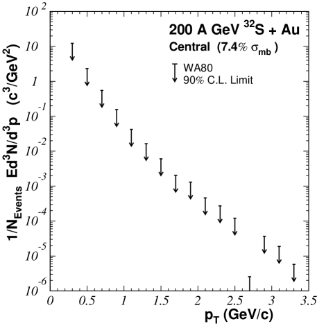
Figure 24: Upper limits ($90\%$ CL) of the direct photon multiplicity as a function of $p_{T}$ in central reactions of ${}^{32}S$ + $Au$ for $\sqrt{s}=19.4\,\mathrm{GeV}$.

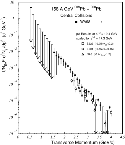
Figure 25: Invariant direct photon multiplicity as a function of $p_{T}$ in central reactions of $Pb$ + $Pb$ for $\sqrt{s}=17.3\,\mathrm{GeV}$. The error bars correspond to combined statistical and systematic errors, the data points with downward arrows indicate $90\%$ CL upper limits. For comparison scaled direct photon results from $p$-induced reaction are included (see text).

The WA80 experiment has performed measurements with ${}^{16}O$ [176] and ${}^{32}S$ [156] beams using a lead glass calorimeter for photon detection. Most hadrons deposit very little energy and are thus effectively suppressed. A shower shape discrimination further reduces the hadron background, and charged hadrons are in addition rejected by the help of a charged particle veto detector consisting of streamer tubes with pad readout. The contamination by neutrons and antineutrons is estimated by Monte Carlo simulation — it is expected to be small. The raw spectra are corrected for a multiplicity dependent reconstruction efficiency. The systematic errors are checked by performing the analysis with a number of different choices of experimental cuts. Inclusive photons and $\pi^{0}$ and $\eta$ mesons have been measured in the same data samples, which helps to control the systematic errors. WA80 reports no significant direct photon excess over decay sources in peripheral and central collisions of ${}^{16}O$ + $Au$ and ${}^{32}S$ + $Au$. The average excess in central ${}^{32}S$ + $Au$ collisions in the range $0.5\,\mathrm{GeV}/c\leq p_{T}\leq 2.5\,\mathrm{GeV}/c$ is given as $5.0\%\pm 0.8\%$ (statistical) $\pm 5.8\%$ (systematic). A $p_{T}$ dependent upper limit ($90\%$ CL) of direct photon production as shown in Fig. 24 has been obtained, which gives more information than the integrated limits, as it can constrain predictions at higher $p_{T}$, where a considerable direct photon multiplicity may be expected.

For $Pb$ + $Pb$ collisions at 158 $A$ GeV ($\sqrt{s_{NN}}=17.3\,\mathrm{GeV}$) the WA98 experiment has performed photon measurements [157] using similar detectors and analysis techniques as WA80. In peripheral collisions no significant direct photon excess was found. In central collisions the observed photons cannot entirely be explained by decay photons, implying the first observation of direct photons in high energy heavy-ion collisions. The extracted direct photon spectrum is shown in Fig. 25. The only other direct photon measurements at a similar energy are from $p$-induced reactions as discussed in Section 3.2.1. Data from $pp$ reactions by E704 [155] and from $p$+$C$ reactions by E629 [164] and NA3 [169] at $\sqrt{s}=19.4\,\mathrm{GeV}$ have been converted to the lower energy $\sqrt{s}=17.3\,\mathrm{GeV}$ assuming a scaling according to Eq. (29) and have been multiplied with the average number of binary nucleon-nucleon collisions in the central $Pb$ + $Pb$ reactions (660). These scaled $p$-induced results are included in Fig. 25 for comparison. They are considerably below the heavy-ion results which indicates that a simple scaling of prompt photons as observed in $pp$ is not sufficient to explain the direct photons in central $Pb$ + $Pb$ reactions. Interpretations of this discrepancy will be discussed in the following chapter.

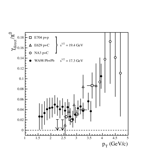
Figure 26: $\gamma_{direct}/\pi^{0}$ ratio as a function of $p_{T}$ for $pp$ and $pC$ reactions $\sqrt{s}=19.4\,\mathrm{GeV}$ as in Fig. 23 (open symbols) and for central $Pb$ + $Pb$ reactions at $\sqrt{s}=17.3\,\mathrm{GeV}$ (filled symbols).

We would like to close our discussion of existing direct photon data by comparing the $\gamma/\pi^{0}$ ratio extracted from heavy-ion data to those from $pp$ and $pC$ in Fig. 26. The value in heavy-ion data is $\approx 3-5\%$ in most of the $p_{T}$ range, which is similar to the lowest values extracted in the proton data. This may be taken as a hint that such levels of direct photons approach the feasibility limit of such measurements. Still lower levels will be very hard or impossible to detect.

3.3 Outlook for RHIC and LHC

In summer 2000 experiments at the Relativistic Heavy Ion Collider (RHIC) at BNL started to take data in collisions of Au nuclei at $\sqrt{s_{NN}}=130\,\mathrm{GeV}$, continuing with a beam energy of $\sqrt{s_{NN}}=200\,\mathrm{GeV}$ from 2001 on. First results of the RHIC experiments have already been presented [8], however results on direct photons are not available at this early stage.

One of the major goals of the PHENIX experiment [177, 178] at RHIC is the measurement of direct photons in the central detector arms at midrapidity. Photon measurements and neutral meson reconstruction are performed with electromagnetic calorimeters using two different technologies, a lead glass detector, which consists of the transformed and updated calorimeter used in WA98 and a lead-scintillator sampling calorimeter. In addition, the sophisticated electron detection capabilities should also allow to measure inclusive photons via the e⁺-e^--pairs from conversions. The central detectors cover $90^{\circ}$ in azimuth and the pseudorapidity range $|\eta|<0.35$. A central magnet provides an axial field, and tracking and momentum measurement is performed in three different sub-systems: pad chambers (PC), drift chambers (DC) and time-expansion chambers (TEC). Electron identification is achieved by simultaneously using a ring imaging Cherenkov counter (RICH) for $p<4.7\,\mathrm{GeV}/c$, electromagnetic energy measurement in the calorimeters for $p>0.5\,\mathrm{GeV}/c$ and $dE/dx$ measurement in the TEC for $p<2\,\mathrm{GeV}/c$. A planned upgrade of the TEC to a transition radiation detector (TRD) will further strengthen the electron identification. Photons converting in the outer shell of the multiplicity and vertex detector (MVD) can be identified as electron pairs with a small, but finite apparent mass. It is planned to add a converter plate to the experiment for part of the data taking to minimize uncertainties of the conversion probability and the location of the conversion point. Photons with $p>1\,\mathrm{GeV}/c$ will be identified in the calorimeters with hadron suppression from the smaller deposited energy and additional rejection by time-of-flight (for slow hadrons) and shower shape analysis. Furthermore, charged hadrons will be identified by the tracking detectors in front of the calorimeters. The calorimeters will also measure $\pi^{0}$ and $\eta$ production necessary for the estimate of the decay photon background.

The different technologies should provide an excellent measurement of direct photons with independent checks of systematic errors. In addition, as RHIC is a dedicated heavy-ion accelerator, a much higher integrated luminosity is expected, which, together with the expected higher photon production rates, will make the RHIC measurements superior to the existing lower energy heavy-ion data.

Pb beams at even higher energies ($\sqrt{s_{NN}}=5.5\,\mathrm{TeV}$) will be available at the future Large Hadron Collider at CERN, which is supposed to deliver heavy-ion beams to physics experiments in 2007. There will be one dedicated heavy-ion experiment, ALICE [179], which is planning to measure direct photons. In addition, one of the $pp$ experiments, CMS [180, 181] may also attempt to measure direct photons at very high transverse momenta in heavy ion collisions. Of course, as LHC is primarily a proton machine and the heavy-ion beam time will be limited, the measurement conditions are not as favorable as at RHIC, the expected photon rates, however, should still be higher and compensate partially for this.

The photon measurement in ALICE will be performed with the photon spectrometer PHOS [182], which consists of a calorimeter out of $PbWO_{4}$ crystals read out by avalanche photodiodes. $PbWO_{4}$ has recently received a lot of attention as a relatively radiation hard, dense crystal suited for photon detection at colliders — it will also be used for the electromagnetic calorimeter of the CMS experiment. The dense material allows to use small cross sections of individual modules and thus yields excellent position resolution and low double hit probability. The energy resolution of the detector is expected to be below $2\%$ for $E_{\gamma}>4\,\mathrm{GeV}/c$. The detector will be operated at $T=-25^{\circ}\mathrm{C}$, which results in a considerably higher light output compared to room temperature. It will cover $|\eta|<0.12$ and $100^{\circ}$ in azimuthal angle. Different options of using either a charged particle veto detector or a pre-shower detector in front of PHOS are still being investigated. A pre-shower detector would provide much better hadron rejection capabilities at higher costs compared to a pure charged particle veto.

The dynamic range of the photon measurements at RHIC should extend over the range $1.0\,\mathrm{GeV}/c\leq p_{T}\leq 30\,\mathrm{GeV}/c$, discrimination of high $p_{T}$ photons from merging $\pi^{0}$ should be possible up to $p_{T}=25\,\mathrm{GeV}/c$. The ALICE PHOS has been optimized for photons in the range $0.5\,\mathrm{GeV}/c\leq p_{T}\leq 10\,\mathrm{GeV}/c$, while measurements should be possible up to $p_{T}=40\,\mathrm{GeV}/c$ with $\pi^{0}$ rejection at least up to $p_{T}=30\,\mathrm{GeV}/c$.

4 Comparison of Theory and Experiment

4.1 Comparisons of prompt photons in $pp$ and $pA$ collisions

The inclusive production of prompt photons in $pp$ collisions is not fully understood [102], as we mentioned already in Section 2.1.3. Using perturbative QCD together with an “optimization” prescription [93], in which the renormalization scale $\Lambda_{\rm QCD}$ and parameters of the parton structure functions are optimized, an excellent agreement between theory [183, 184, 185, 186] and experiments until 1997 [92] over the entire range of collision energy $\sqrt{s}$ and transverse photon momentum $p_{T}$ was obtained, choosing a single set of structure functions and a unique value for $\Lambda_{\rm QCD}$. However, new data from E706 ($p-Be$ and $\pi-Be$) at $\sqrt{s}=31.6$ GeV and $\sqrt{s}=38.8$ GeV [91] cannot be explained in this way, as shown in Fig. 27.

Figure 27: Normalized ratio of data to theory for various experiments as a function of $x_{T}=2p_{T}/\sqrt{s}$ [102].

The disagreement between theory and experiment persists even if the theoretical description is improved by a soft-gluon resummation and by including next-to-next-to-leading-order corrections [94]. An agreement between theory and data can be achieved only by introducing an intrinsic transverse parton momentum $k_{T}$ as a new phenomenological energy-dependent parameter [96, 97]. However, choosing $k_{T}=0.7$ GeV for fitting the UA6 data and $k_{T}=1.2$-1.3 GeV for E706 implies $k_{T}>1.5$ GeV for the ISR data, which destroys the agreement with data sets of WA70 and ISR [102]. On the other hand, for the $pA$ data from E706 the introduction of an additional $k_{T}$ broadening by nuclear effects (Cronin effect [88]) provides a possible explanation of the data [99] as shown in Fig. 28.

Figure 28: Comparison of data from E706 with theoretical calculations with (solid line) and without (dashed line) Cronin effect [99].

Similarly, Wong and Wang [100] concluded that most experimental data can be explained if an intrinsic transverse momentum of the partons is taken into account. For example, at $\sqrt{s}=19.4$ GeV the photon invariant cross section is enhanced by a factor of 2 if next-to-leading order corrections are included and by a factor of 4 to 8 due to the transverse momentum effect (see Fig. 29). Also shown is the small influence of using different parametrizations (DO, CTEQ, MRS96) of the parton distributions on the cross section.

Figure 29: Comparison of data at $\sqrt{s}=19.4$ GeV with theoretical calculations using next-to-leading order corrections (NLO), an intrinsic transverse momentum (PT), and different parton distributions (DO, CTEQ, MRS96) [100].

Furthermore, Apanasevich et al. [187] compared theoretical models including next-to-leading order and intrinsic momentum effects with ratios of $\gamma/\pi^{0}$ yields, in which various experimental and theoretical uncertainties cancel. They conclude that the theory agrees reasonably with data at $\sqrt{s}>30$ GeV, whereas at lower energies deviations between theory and experiments as well as between different data sets appear.

4.2 Comparison with SPS Heavy-Ion Experiments

4.2.1 Comparison to Limits of WA80

The first confrontations of theoretical calculations [129, 188, 189, 190, 191] to experimental heavy-ion data were performed with the preliminary WA80 data [192] which indicated a significant excess of direct photons in central $S$+$Au$ reactions. We will not discuss this in detail, as the final publication of the WA80 data [156] did only provide an upper limit for direct photon production. All of these publications have been able to describe the preliminary WA80 data with scenarios including a phase transition using 1-loop HTL rates for the QGP. To achieve this, Shuryak and Xiong [188] had to assume a surprisingly long-living mixed phase. Furthermore, Srivastava and Sinha [129] and Dumitru et al. [191] concluded that a pure hadron gas scenario could be excluded because it would overpredict the observed photon spectra. While the interpretation found in Ref. [188] could no longer be sustained from the final WA80 data, the conclusions of Refs. [129] and [191] are related to some of the simplifying assumptions, mainly the unrealistic equation of state used for the HHG.

Figure 30: Comparison of the WA80 upper limits [156] with hydrodynamical calculations using different EOS [193]. EOS A and B contain a phase transition, EOS H corresponds to a HHG of massive mesons and baryons and EOS I to an ideal pion gas.

Figure 31: Comparison of photon spectra with a simplified HHG EOS (left) and a realistic one (right) [195].

Sollfrank et al. [193] employed a 2+1-dimensional hydrodynamical model to calculate hadronic and electromagnetic spectra at the same time. They investigated various EOS with and without phase transition. They concluded that the WA80 limits only exclude an ideal pion gas for the EOS of the HHG. A no-phase-transition scenario with a more complicated HHG EOS, on the other hand, is not ruled out (see Fig. 30) for initial temperatures below $T_{0}=250$ MeV. Also in Ref. [194], it was found that the WA80 upper limits for direct photons cannot distinguish between a phase transition and no phase transition. Furthermore, it was argued that medium effects on hadron masses will reduce the high $p_{T}$ spectrum by about a factor of 2.

Recently, Srivastava and Sinha repeated their calculations using the 2-loop HTL results [49, 51] and a HHG EOS with all hadrons with masses up to 2.5 GeV [195, 196]. The importance of a realistic EOS for the HHG, discussed already in Section 2, is demonstrated in Fig. 31, where one observes that a HHG EOS with only $\pi$-, $\rho$-, $\omega$-, and $\eta$-mesons leads to a large overprediction of the photon spectrum at SPS energies, whereas a realistic EOS including hundreds of resonances is similar to the spectrum with a phase transition. The new conclusion by Srivastava and Sinha was that the phase transition as well as the no-phase transition scenario agree with the upper limits from WA80 [197] (see Fig. 32). However, they argue that a hadron density of several hadrons per fm³ is needed at the initial time, which seems to contradict the assumption of a HHG.

Summarizing, the upper limits for direct photons from WA80 can be explained with and without phase transition and, therefore, do not allow a conclusion about the existence of a QGP phase. However, they have triggered investigations of some of the simplifications used in earlier calculations, as e.g. unrealistic EOS for the HHG.

Figure 32: Comparison of the WA80 upper limit [156] for the direct photon spectrum to a calculation with (left) and without (right) phase transition [197].

4.2.2 Comparison with WA98

Recently the WA98 Collaboration presented the first data on direct photons in relativistic heavy-ion collisions [157]. Different groups comparing their calculations with these data arrived at different conclusions, which we will review in the following.

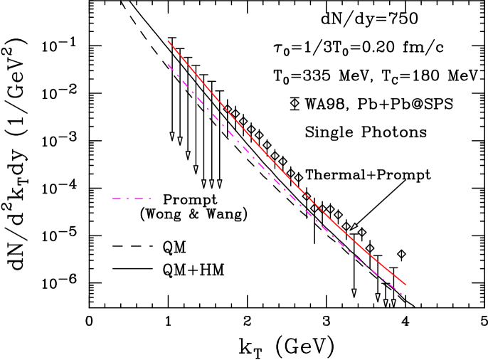
Figure 33: Comparison of the WA98 data with a hydrodynamical calculation by Srivastava and Sinha [127].

Srivastava and Sinha [127] argued, using the 2-loop HTL rate for the QGP contribution and a realistic EOS for the HHG, that the QGP is needed to explain the data. Their conclusion is based on the use of a very high initial temperature ($T_{0}=335$ MeV) and very small initial time ($\tau_{0}=0.2$ fm/c), which could explain the observed flat photon spectrum for transverse photon momenta $p_{T}>2$ GeV (see Fig. 33). Their estimate of the initial conditions follows from the isentropy condition Eq. (17) [20] together with the use of the uncertainty principle [122], $\tau_{0}\simeq 1/3T_{0}$. However, the uncertainty relation, giving the parton formation time, might underestimate the thermalization time [122]. However, the authors argue that such a small thermalization time also provides a very good description of the intermediate mass dilepton excess measured by NA50 [198]. Also, if later thermalization times are assumed, one should add a pre-equilibrium contribution to the photon spectrum. Using more conservative initial conditions ($T_{0}=196$ MeV, $\tau_{0}=1$ fm/c), the data are clearly underestimated in particular at $p_{T}>2$ GeV (see Fig. 34). Srivastava and Sinha have also included prompt photons from the work by Wong and Wang [100], which follow from a next-to-leading order perturbative QCD calculation, where an intrinsic parton momentum of $\langle k_{T}^{2}\rangle=0.9$ GeV² has been used. Srivastava and Sinha found that the thermal photons contribute half of the total photon spectrum and that in particular at large $p_{T}$ most of the thermal photons are due to the QGP contribution. However, one should keep in mind that the question of the QGP photon rate is not yet settled and that the 2-loop HTL calculation might be an overestimation, since the LPM-effect is neglected there [63]. Furthermore, Srivastava and Sinha neglected a finite baryo-chemical potential, which reduces the QGP contribution to the photon spectrum. For example, even a small baryo-chemical potential of $\mu_{B}=100$ MeV, corresponding to a quark-chemical potential $\mu_{q}=300$ MeV, reduces the 1-loop HTL photon production rate by more than a factor of 3 at $p_{T}=3$ GeV [43]. On the other hand, the photon production from nucleons and other baryons might enhance the rate [79].

Figure 34: Comparison of the SPS photon and pion spectra with hydrodynamical calculations using different initial times [127]. $\tau_{0}=0.2$ fm/c corresponds to the upper lines.

Also Alam et al. [199] favor a QGP contribution for explaining the WA98 data. However, they claim that due to the uncertainties in the rates and the hydrodynamical parameters a definite conclusion is not possible at SPS energies. Alam et al. used a EOS of the HHG with much less degrees of freedom than Srivastava and Sinha. However, they considered in-medium modifications of hadron masses which lead to an enhancement of the photon spectrum at SPS energy for photon momenta above $p_{T}=2.5$ GeV. At $p_{T}=4$ GeV this enhancement amounts to an order of magnitude. In addition, they introduced an initial radial velocity $v_{0}$, which renders the photon spectrum flatter at $p_{T}>2$ GeV even for moderate values of $v_{0}=0.2c$. Owing to these effects, Alam et al. obtained a much flatter spectrum at high $p_{T}$, which allows an explanation of the WA98 data without prompt photons within the phase-transition as well as the no-phase-transition scenario, even for conservative initial conditions, $T_{0}\simeq 200$ MeV and $\tau_{0}=1$ fm/c. However, in a number of papers hydrodynamical calculations were able to reproduce hadronic as well as electromagnetic spectra (see e.g. [123]) and flow patterns [200, 201] without assuming an initial radial velocity. In particular, the high $p_{T}$ component above 2 GeV in the $\pi^{0}$-spectrum, which has been used to argue about an initial radial velocity [202], might also come from hard processes and should not be treated in a hydrodynamical model [203].

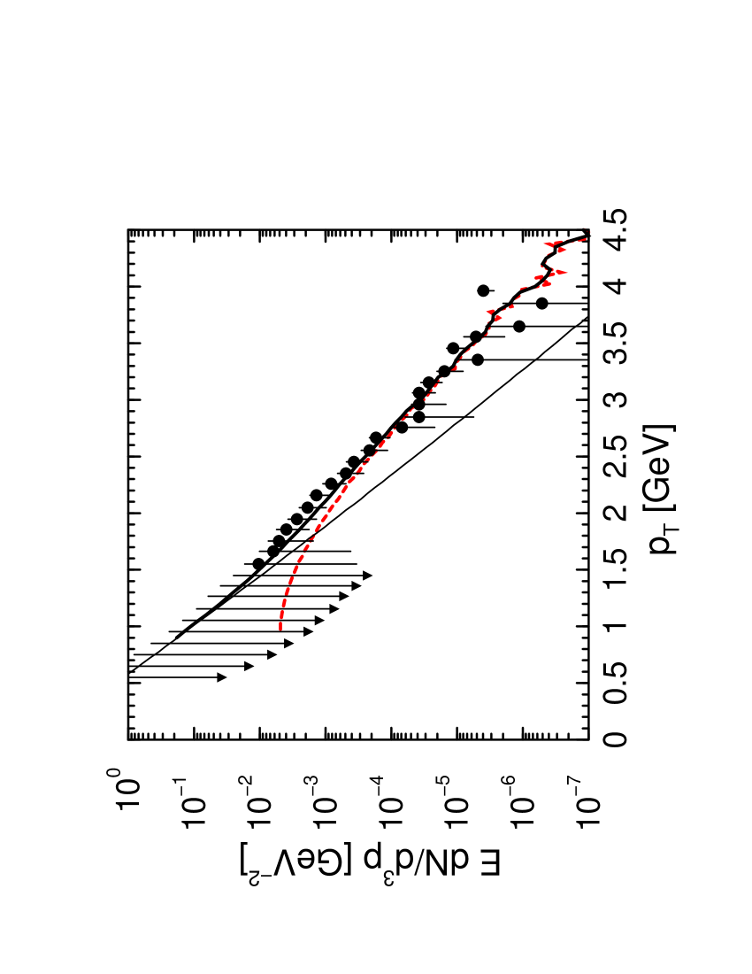
Figure 35: Comparison of the WA98 data with a theoretical spectrum (upper solid line) including thermal (lower solid line) and prompt photons (dashed line) [73].

Gallmeister et al. [73], on the other hand, argued that the low momentum part of the WA98 spectrum ($p_{T}<2$ GeV) is consistent with a thermal source, either QGP or HHG, which also describes dilepton data. The hard part ($p_{T}>2$ GeV), on the other hand, agrees with the prompt photon spectrum if its absolute value is normalized to the data, corresponding to a large effective $K$-Factor of 5 (see Fig. 35). It should be noted that the prompt photon production at $\sqrt{s}=17.3$ GeV is uncertain, in particular for low $p_{T}$. Gallmeister et al. used a simple hydrodynamical model with only a radial expansion and a fixed average temperature, which reproduces dilepton data from SPS [204]. In addition, they adopted only the 1-loop HTL rate for the entire evolution of the fireball according to the quark-hadron duality hypothesis. If in addition a transverse flow of $v=0.3$ is included, the theoretical and experimental spectra agree. In other words, according to the investigation by Gallmeister et al., the WA98 spectrum can be explained by a thermal source (QGP or HHG) plus prompt photons and there is no necessity of a QGP phase. Similarly, Dumitru et al. [90] showed that the WA98 photon spectrum above $p_{T}=2.5$ GeV can be explained by prompt photons if a nuclear broadening of $\Delta k_{T}^{2}=\langle k_{T}^{2}\rangle_{AA}-\langle k_{T}^{2}\rangle_{pp}\simeq 0.5$ - 1 GeV² is introduced. For low $p_{T}<2.5$ GeV, however, prompt photons fail to reproduce the WA98 data regardless of the amount of nuclear broadening employed (see Fig. 36).

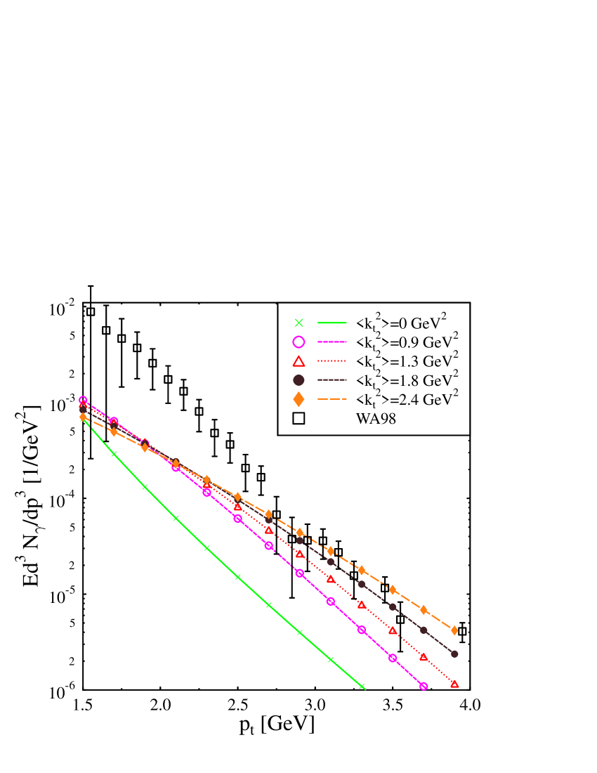
Figure 36: The photon spectrum calculated for different intrinsic transverse momenta in comparison to the WA98 data [90].

Figure 37: The photon spectrum calculated for different EOS and initial conditions with prompt photons (upper set, scaled by a factor 100) and without (lower set) in comparison to the WA98 data [205]. EoS A, IS 1 contains a phase transition at $T_{c}=165$ MeV, an average initial temperature $T_{0}=255$ MeV, and a local maximum temperature $T_{\rm max}=325$ MeV. EoS H describes only a HHG with $T_{0}=234$ MeV, $T_{\rm max}=275$ MeV (IS 1) and $T_{0}=213$ MeV, $T_{\rm max}=245$ MeV (IS 2).

Huovinen et al. [123], fixing the initial conditions ($T_{0}=210$ - 250 MeV) in their hydrodynamical model partly by a comparison with hadron spectra and using the most recent results for the QGP photon rate by Arnold et al. [66], were able to describe the data equally well with or without a phase transition [205] (see Fig. 37). They were able to fit the WA98 data without a high initial temperature, an initial radial velocity, prompt photons, or in-medium hadron masses. This might be caused partly by a strong flow at later stages since they do not assume a boost-invariant longitudinal expansion. However, the different results and conclusions between the work by Srivastava and Sinha [127] and by Huovinen and Ruuskanen [205] cannot be explained in this way [206]. The conclusion, that the WA98 data can be explained with or without a phase transition, was also obtained in Refs.[202, 207]. However, there an initial radial velocity (see above) had to be introduced in order to obtain a quantitative description of the WA98 data.

Steffen and Thoma [51], using the corrected 2-loop HTL rate, the parametrization of the HHG rate Eq. (11), and the simple 1-dimensional Bjorken hydrodynamics, found that the thermal photons underestimate the WA98 data for $p_{T}>2$ GeV for reasonable initial temperatures between 170 and 235 MeV (see Fig. 38). These high $p_{T}$ photons, however, might be explained by prompt photons. Using a massless pion gas ($g_{h}=3$) for the HHG EOS, the computed spectrum exceeds the WA98 data at $p_{T}<2$ GeV already for initial temperatures as low as $T_{0}=170$ MeV. However, if one increases the number of massless pions to $g_{h}=8$, which provides an agreement with photon spectra from the HHG using more realistic EOS [127], the life-time of the mixed phase is shortened, which allows higher initial temperatures, up to $T_{0}=235$ MeV.

Figure 38: The photon spectrum calculated for different critical and initial temperatures and degrees of freedom in the HHG in comparison to the WA98 data [51].

Summarizing, WA98 found a rather flat photon spectrum above $p_{T}=2$ GeV, which cannot be easily explained by conservative models. It requires either a high initial temperature, a large prompt photon contribution, an initial radial velocity, in-medium modifications of the hadron masses and/or a strong flow at later stages. Furthermore, the effect of a finite baryo-chemical potential, which should be important at SPS energies, has not been investigated so far. Also the effect of a finite life-time of the QGP, which flattens the high $p_{T}$ spectrum [139, 140], has only be considered for RHIC energies (see below). At the moment, we think it is fair to say that the uncertainties and ambiguities in the hydrodynamical models and in the rates do not allow to decide from the WA98 photon spectra about the presence of a QCD phase transition in SPS heavy-ion collisions.

4.3 Predictions for RHIC and LHC

There are a few predictions for the photon spectra for RHIC and LHC. Although they suffer from large uncertainties coming from the unknown initial conditions, at least for LHC in most cases a window in the photon momentum is predicted, where a thermal QGP contribution should be visible if the decay photons are subtracted. Simple 1+1-dimensional models [51, 126] show a dominance of the QGP over the hadron gas contribution for $p_{T}>3$ GeV (RHIC) and $p_{T}>2$ GeV (LHC), respectively, due to the flat spectrum of the early QGP phase having a high initial temperature ($T_{0}>300$ MeV), as shown in Fig. 39.

Figure 39: QGP and HHG photon spectra at SPS, RHIC and LHC $Pb+Pb$ collisions for an ideal pion gas with $g_{h}=3$ (left) and $g_{h}=8$ (right) degrees of freedom [51].

Taking into account the transverse expansion, the photon spectrum from the hadron gas becomes also flat due to a strong flow in the late stages of the fireball. But even in this case, the QGP might outshine the hadronic phase. However, at which collision energies and photon momenta this happens, is controversial. Hammon et al. [208] predict that the QGP should not be visible at RHIC, where the prompt photons dominate the spectrum, but at LHC for $p_{T}\simeq 2$-5 GeV. They used the following initial conditions for RHIC, $T_{0}=533$ MeV and 300 MeV and $\tau_{0}=0.1236$ fm/c and 0.5 fm/c, and for LHC, $T_{0}=880$ and 650 MeV and $\tau_{0}=0.1$ fm/c and 0.25 fm/c, together with a simple HHG EOS and the 1-loop HTL result for the QGP and HHG rates.

Srivastava [209], taking into account the corrected 2-loop HTL rate, predicts that the QGP should be observable for $p_{T}<1$ GeV at RHIC and $p_{T}<2$ GeV at LHC (see Fig. 40). Above these momenta the sum of the photons from the thermal hadron gas, enhanced by flow, and of the prompt photons dominates. Using the old 2-loop HTL rate, which is too large by a factor of 4, Srivastava found that the QGP photons dominate already for $p_{T}<3$ GeV at RHIC and $p_{T}<4$ GeV at LHC, which shows the sensitivity of the predictions to the rates.

Peressounko and Pokrovsky [141] predict a ratio of direct to decay photons of 0.2-0.3 at LHC, which is much larger than the 5% limit for direct photons to be detectable at ALICE. Whether the photons from the QGP or from the HHG dominate, depends on rates that are adopted in their calculations.

Alam et al. [199], using $T_{0}=300$ MeV, $\tau_{0}=0.5$ fm/c together with the incorrect 2-loop HTL rate for the QGP, predict that for $p_{T}<2$ GeV most of the photons are thermal photons. The photons from the QGP are an important source, in particular around 2 GeV, but less important than HHG photons. The effect of the transverse expansion is small in the QGP phase but large in the late stages of the HHG, leading to a strong population of high $p_{T}$ photons together with prompt photons.

Dumitru et al. [90] have investigated the role of prompt photons at RHIC. They showed that the effect of an intrinsic $k_{T}$ is less important at RHIC than at SPS, but still leads to an enhancement of the prompt photons by a factor of 3 at $p_{T}=3$-4 GeV. Below $p_{T}<2$-3 GeV thermal photons should be visible.

All these investigations did not take into account deviations from a chemical equilibrium, which could be important at RHIC and LHC [114]. In particular, a gluon dominated, hot early phase is expected, in which quarks are strongly suppressed compared to their equilibrium abundance [135]. This would lead to a suppression of about two orders of magnitude of high $p_{T}$ photons from the QGP. However, extending the rates as well as the hydrodynamical model to chemical non-equilibrium, one observes that this strong suppression is compensated to a large extent by the much higher initial temperature of the dilute parton gas compared to an equilibrated QGP at the same initial energy density, as shown by Mustafa and Thoma [52] (see Figs. 41 and 42). Here a transverse expansion was included, and initial conditions for the temperature and the fugacities from the self-screened parton cascade model (SSPC) [210] ($T_{0}=668$ MeV, $\lambda_{g}^{0}=0.34$, $\lambda_{q}^{0}=0.064$ for RHIC and $T_{0}=1020$ MeV, $\lambda_{g}^{0}=0.43$, $\lambda_{q}^{0}=0.082$ for LHC) together with a Fermi-like nuclear profile have been used. At RHIC, the non-equilibrium compared to the equilibrium photon spectrum is suppressed by a factor of 5 at $p_{T}=1$ GeV but enhanced by a factor of 2 at 5 GeV. At LHC, the non-equilibrium yield is smaller by about a factor of 3 for all momenta. Note that in the non-equilibrium case the annihilation-with-scattering contribution to the 2-loop HTL rate is largely reduced because it has at least two quarks in the initial channel, which are suppressed by the small quark fugacities. Hence, the relative importance of the various contributions (Compton, annihilation, bremsstrahlung, and annihilation-with-scattering) is different in the non-equilibrium compared to the equilibrium scenario. Also prompt photons have been included (see Figs. 41 and 42), and a dominance of the thermal contribution over the prompt photons for $p_{T}<3.5$ GeV at RHIC and LHC has been found.

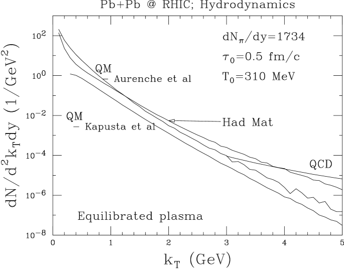
Figure 40: Predictions for the photon spectrum at RHIC (left) and LHC (right) [209].

It should be noted, however, that predictions of the photon yield at RHIC and LHC suffer also from a large uncertainty in the initial conditions (temperature, quark and gluon fugacities) for the chemical equilibration, which are predicted very differently in different transport models. For example, the HIJING model [121] predicts much smaller initial temperatures and fugacities, which lead to a much stronger suppression of the photon yield in the non-equilibrium case [52].

Moreover, effects of the finite life-time of the QGP, leading to a strongly enhanced non-exponential photon spectrum at high $p_{T}$, could help to identify the QGP contribution at RHIC and LHC [139, 140].

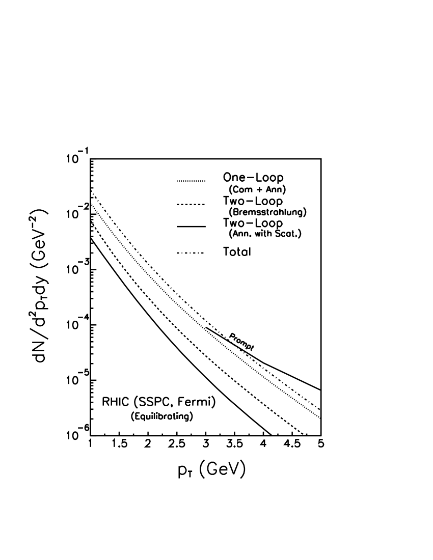
Figure 41: Comparison of the the photon spectrum at RHIC from an equilibrated QGP (left) and a chemically non-equilibrated QGP (right) at the same initial energy density $\epsilon_{0}=61.4$ GeV/fm³ [52].

Figure 42: Comparison of the the photon spectrum at LHC from an equilibrated QGP (left) and a chemically non-equilibrated QGP (right) at the same initial energy density $\epsilon_{0}=425$ GeV/fm³ [52].

It is interesting to note that at SPS even simple hydrodynamical models without a phase transition work due to the small life-time of the QGP phase [73]. At RHIC and LHC, on the other hand, we expect that the QGP contribution becomes significant, which might allow to distinguish between hydrodynamical calculations using different EOS, initial conditions and photon rates as input.

In conclusion, the transverse expansion of the later stages in the HHG phase is important at RHIC and LHC and renders the photon spectrum rather flat at large $p_{T}$. Hence the hot QGP contribution to the spectrum, presuming the formation of a QGP phase, will be covered partly by these HHG photons and prompt photons. Whether there is a $p_{T}$ window, where the QGP photons dominate depends on details of the rates and the hydrodynamical models, which are not yet under control. Hadronic and dilepton spectra will help to reduce these uncertainties by constraining the initial conditions. Anyway, the QGP contribution to the photon spectrum at RHIC and LHC will be significant and might be extracted from the observed spectra by comparing with calculations. Moreover, the experimental photon spectra at RHIC and LHC will provide interesting information on the initial conditions and the chemical equilibration of the fireball.

5 Summary and Conclusions

Energetic photons from high-energy hadronic and nucleus-nucleus collisions provide important information about fundamental aspects of the particles involved and their interactions. In particular, they probe the parton distributions in hadrons and nuclei. In relativistic heavy-ion collisions, they serve as a direct probe for all stages of the fireball since they leave the system without further interactions due to their large mean free path. Most important, the thermal radiation from the fireball might allow to extract information on the EOS of the matter produced in the collision. Hence, the direct photon production provides one of the most promising signatures for the QGP, a new state of matter likely to be created in ultrarelativistic heavy-ion collisions.

Direct photons have been observed in $pp$ and $pA$ reactions at collision energies from $\sqrt{s}=19.3$ GeV to 1.8 TeV. In these experiments, they can be distinguished from the decay photons, coming from hadronic decays, within the experiment directly. At the present stage, the results for direct photons are controversial, especially at low collision energies.

Direct photons from high-energy nucleus-nucleus collisions cannot be identified experimentally due to the high hadron multiplicity. Rather, one has to subtract the dominating background of the decay photons by reconstructing them from the measured hadrons, mainly $\pi^{0}$ and $\eta$. In this way, WA98 were able to observe direct photons at the SPS in central $Pb+Pb$ collisions at a beam energy of 158 GeV per nucleon, corresponding to $\sqrt{s_{NN}}=17.3$ GeV, whereas WA80 gave only an upper limit for direct photons in $S+Au$ collisions at a beam energy of 200 A GeV. The extracted direct photon spectrum from WA98 shows a clear excess over the background for photon transverse momenta between 1.5 and 3.5 GeV/c.

In order to learn from these experimental results about the hadrons and their interactions, one has to compare them to theoretical pre- and postdictions. In $pp$ and $pA$ collisions the cross sections for prompt photon production have been calculated within perturbative QCD. These cross sections follow from folding the basic partonic processes, e.g. $q\bar{q}\rightarrow g\gamma$, with the parton distributions of the hadrons. Using next-to-leading or even next-to-next-to-leading order corrections plus an optimization procedure for fixing the parameters (renormalization and factorization scales), a reasonable description of most of the data can be obtained although there are some clear discrepancies in particular at low collision energies. Assuming an intrinsic momentum broadening in the parton distributions, a better agreement with the various data sets can be obtained, of course at the expense of introducing a new parameter. Indications for an additional nuclear broadening (Cronin effect) have also been found in $pA$ collisions.

In a spatially and temporally extended system like the fireball in a nucleus-nucleus collision, it is not sufficient to compute the cross sections or rates for photon production. Rather, one has to convolute the rates with the space-time evolution of the fireball, for which usually hydrodynamical models are adopted. Furthermore, one has to consider the photon production from different stages, i.e. prompt photons from initial hard collisions and thermal photons from the QGP and the HHG. In this way, photon spectra are obtained which can be compared to experimental spectra. In order to draw a conclusion on the possible presence of a QGP phase, one has to compare predictions for spectra with and without a QGP phase to experimental results.

The calculation of the photon production rate from an equilibrated (or chemically non-equilibrated) QGP is based on perturbative QCD at finite temperature. To lowest order the basic processes are quark-antiquark annihilation and Compton scattering. Owing to infrared singularities the HTL resummation technique has to be employed. Assuming the weak coupling limit, the leading logarithm contribution can be extracted in this way. However, beyond the leading logarithm infinitely many diagrams, corresponding for example to bremsstrahlung, contribute to the same order. Hence, the photon production rate from the QGP beyond the leading logarithm approximation may not be perturbatively describable. In the most recent calculations of photon spectra, the 2-loop rate within the HTL improved perturbation theory has been used as an educated guess. The photon production rate from the HHG, on the other hand, is based on effective models for hadronic interactions. The most important contributions to the rate come from interactions between $\pi$- and $\rho$-mesons. In particular, the $a_{1}$ resonance plays an important role for the photon production. Also the HHG rate suffers from a number of uncertainties such as assumptions about the effective Lagrangians, medium effects, etc.

For deriving the spectra from the rates, various hydrodynamical models, describing the expansion of the fireball in 1, 2 or 3 spatial dimensions, fixing the initial conditions in different ways, using different EOS, and including a chemically non-equilibrated QGP have been employed. However, a systematic and comprehensive treatment is still missing. In other words, theoretical predictions are subject to uncertainties in the rates as well as the hydrodynamical description.

The present calculations do not allow to infer about the existence of a QGP phase in central $Pb+Pb$ collisions at a beam energy of 158 A GeV. However, the data are consistent with a thermal source, either QGP or HHG, for photons with $p_{T}<2.5$ GeV/c and with enhanced prompt photons for $p_{T}>2.5$ GeV/c.

The situation will change drastically at RHIC and LHC. The RHIC experiments including PHENIX with its excellent photon detection have started to take data at $\sqrt{s_{NN}}=200$ GeV. They will measure photon spectra with very high statistics. The ALICE experiment planned for the CERN LHC is gearing up to measure photons in heavy-ion reactions at still higher beam energy. A much larger temperature and life-time of the fireball in these collisions will cause a copious production of thermal photons. Most estimates of the photon spectra at RHIC and LHC predict a window around $p_{T}=2$ GeV, where the QGP contribution should dominate. However, in order to confirm this prediction, new developments in the calculation of the rates from QCD as well as a consistent description of the space-time evolution would be essential. This conclusion applies also to all the other signatures for the QGP, as quantitative predictions of non-perturbative QGP properties are required, taking into account the dynamical evolution of the fireball at the same time. Unfortunately, at the moment there is no non-perturbative, dynamical approach to QCD available. Hence, the prospects and problems for discovering the QGP from the direct photon production are similar as for other signatures. However, direct photons from relativistic heavy-ion collisions will definitely help to reveal and understand important and interesting properties of strongly interacting matter.

Acknowledgements:

We would like to thank P. Aurenche, T.C. Awes, A. Dumitru, K. Gallmeister, F. Gelis, K. Haglin, P. Huovinen, B. Kämpfer, P. Levai, M. Mustafa, V. Ruuskanen, D. Srivastava, and H. Zaraket for helpful comments and discussions. We are also grateful to K. Reygers and F. Steffen for their careful reading of the manuscript. M.T. has been supported by the Heisenberg program of the Deutsche Forschungsgemeinschaft. M.T. would also like to thank CERN for its hospitality, where a large part of this work has been performed.

6 Appendix A: Perturbative Calculation of the Photon Production Rate

In this Appendix the photon production rate of energetic photons ($E\gg T$) is derived to lowest order perturbation theory from the diagrams of Fig. 1, corresponding to quark annihilation and Compton scattering. Starting from the definition Eq. (2) of the rate, using the matrix elements for these processes, Kapusta et al. [25] calculated the rate, assuming Maxwell-Boltzmann distributions for the incoming partons, i.e. $n_{i}\sim\exp(-E_{i}/T)$ for $i=1,2$ in Eq. (2). This facilitates the evaluation of the momentum integrals over $p_{1}$ and $p_{2}$ in Eq. (2), which otherwise can be done only numerically. The use of the Boltzmann distribution instead of the exact quantum statistical distributions for quarks and gluons is justified in the case of energetic photons, $E\gg T$. Owing to energy conservation, the sum of the incoming parton energies is much larger than the temperature, $E_{1}+E_{2}=E\gg T$, and the phase space for small $E_{1}$ or $E_{2}$ is unfavorable [25]. Comparing to the numerical calculation using Fermi and Bose distributions, one observes that the error introduced by the Boltzmann approximation is less than a few percent [22].

But even assuming Boltzmann distributions for the incoming particles, the momentum integrations are still rather involved, although they can be performed analytically [21]. However, the calculation can be facilitated further on by computing the inverse process, photon absorption, and using the principle of detailed balance [15, 211]. Accordingly, the photon production rate is related to the photon damping or absorption rate $\gamma$ by [211]

$$\frac{dN}{d^{4}xd^{3}p}=\frac{4}{(2\pi)^{3}}\>e^{-E/T}\>\gamma.$$ (33)

The damping rate is defined as the imaginary part of the dispersion relation $\omega(p)$ of a real photon in the QGP, $\gamma=-{\rm Im}\,\omega(p)$, i.e. it follows from

$$\omega^{2}-p^{2}-\Pi_{T}(\omega,p)=0,$$ (34)

where

$$\Pi_{T}(p_{0},p)=\frac{1}{2}\>\left(\delta_{ij}-\frac{p_{i}p_{j}}{p^{2}}\right)\>\Pi_{ij}(p_{0},p)$$ (35)

is the transverse polarization tensor at finite temperature. ($\Pi_{ij}$ denotes the spatial components of the polarization tensor.) Assuming no overdamping, i.e. $\gamma\ll p$, we find

$$\gamma=-\frac{1}{2p}{\rm Im}\,\Pi_{T}(p_{0}=p,p).$$ (36)

Using cutting rules [23], the damping rate can be calculated alternatively from the matrix elements. In the case of Compton scattering, i.e. the inverse process of the one in Fig. 1, namely photon absorption and gluon emission, the damping rate is given as

$$\gamma_{\rm comp} = \frac{1}{4E}\int\frac{d^{3}p_{3}}{(2\pi)^{3}2E_{3}}\>n_{F}(E_{3})\>\int\frac{d^{3}E_{2}}{(2\pi)^{3}2E_{2}}\>[1+n_{B}(E_{2})]\>\int\frac{d^{3}E_{1}}{(2\pi)^{3}2E_{1}}$$ (37)

$$[1-n_{F}(E_{2})]\>(2\pi)^{4}\>\delta^{4}(P+P_{3}-P_{2}-P_{1})\>\sum_{i}\langle|{\mathcal{M}}|^{2}\rangle_{\rm comp}.$$

In the case of pair creation, i.e. the inverse process of quark-antiquark annihilation in Fig. 1, we have

$$\gamma_{\rm pair} = \frac{1}{4E}\int\frac{d^{3}p_{3}}{(2\pi)^{3}2E_{3}}\>n_{B}(E_{3})\>\int\frac{d^{3}E_{2}}{(2\pi)^{3}2E_{2}}\>[1-n_{F}(E_{2})]\>\int\frac{d^{3}E_{1}}{(2\pi)^{3}2E_{1}}$$ (38)

$$[1-n_{F}(E_{1})]\>(2\pi)^{4}\>\delta^{4}(P+P_{3}-P_{2}-P_{1})\>\sum_{i}\langle|{\mathcal{M}}|^{2}\rangle_{\rm pair}.$$

In Eqs. (37) and (38) the factor $1/(4E)$ instead of the usual $1/(2E)$ comes from the definition of the damping rate as the imaginary photon energy. The sums in front of the matrix elements indicate sums over the initial states of the incoming parton, since all possible states of the partons interacting with the photon have to be counted in the rate. The matrix elements summed over all initial and final parton states are given by [212]

$$\sum_{i}\langle|{\mathcal{M}}|^{2}\rangle_{\rm comp} = -32\>\frac{5}{9}\>e^{2}\>g^{2}\>\left(\frac{u}{s}+\frac{s}{u}\right),$$

$$\sum_{i}\langle|{\mathcal{M}}|^{2}\rangle_{\rm pair} = 16\>\frac{5}{9}\>e^{2}\>g^{2}\>\left(\frac{u}{t}+\frac{t}{u}\right),$$ (39)

where we neglected the quark masses as the bare up and down quark masses are much smaller than the temperature. The Mandelstam variables are $s=(P+P_{3})^{2}$, $t=(P-P_{2})^{2}$, and $u=-s-t$. The factor $5/9$ comes from the sum over the square of the electric charges of the up and down quarks.

The Boltzmann approximation for the incoming particles in the production rate corresponds to using Boltzmann distributions for the outgoing particles in the damping rate. This means that we simply neglect the distribution functions in the Pauli blocking or Bose enhancement factors in Eqs. (37) and (38) since they do not exist in classical statistics. This can also be seen by writing, for example, $1+n_{B}(E_{2})=\exp(E_{2}/T)\,n_{B}(E_{2})\simeq 1$. The advantage compared to the direct calculation of the production rate is now that there are no distributions functions in the momentum integrations over $p_{1}$ and $p_{2}$. Hence we can easily evaluate these integrals by transforming to the center of mass system using the Lorentz invariant phase space factor [212]

$$dL=(2\pi)^{4}\>\delta^{4}(P+P_{3}-P_{2}-P_{1})\>\frac{d^{3}E_{2}}{(2\pi)^{3}2E_{2}}\frac{d^{3}E_{1}}{(2\pi)^{3}2E_{1}}=\frac{dt}{8\pi s}.$$ (40)

Then the integration over $t$ from $-s-\Lambda^{2}$ to $-\Lambda^{2}$, where $\Lambda$ is a cutoff for the logarithmic IR divergence of the $t$ and $u$ channel, leads to

$$\int dL\>\sum_{i}\langle|{\mathcal{M}}|^{2}\rangle_{\rm comp} = \frac{20}{9\pi}\>e^{2}\>g^{2}\>\left(\ln\frac{s}{\Lambda^{2}}+\frac{1}{2}\right),$$

$$\int dL\>\sum_{i}\langle|{\mathcal{M}}|^{2}\rangle_{\rm pair} = \frac{20}{9\pi}\>e^{2}\>g^{2}\>\left(\ln\frac{s}{\Lambda^{2}}-1\right).$$ (41)

The remaining integral over $p_{3}$ can be done using $s=2pp_{3}(1-\hat{p}\cdot\hat{p}_{3})$ and

$$\int_{0}^{\infty}dp_{3}\>p_{3}\>n_{B}(p_{3}) = \frac{\pi^{2}T^{2}}{6},$$

$$\int_{0}^{\infty}dp_{3}\>p_{3}\>n_{F}(p_{3}) = \frac{\pi^{2}T^{2}}{12},$$ (42)

and

$$\int_{0}^{\infty}dp_{3}\>p_{3}\>\ln\frac{p_{3}}{\Lambda}\>n_{B}(p_{3}) = \frac{\pi^{2}T^{2}}{6}\>\left[\ln\frac{T}{\Lambda}+1-\gamma-\frac{\zeta^{\prime}(2)}{\zeta(2)}\right],$$

$$\int_{0}^{\infty}dp_{3}\>p_{3}\>\ln\frac{p_{3}}{\Lambda}\>n_{F}(p_{3}) = \frac{\pi^{2}T^{2}}{12}\>\left[\ln\frac{2T}{\Lambda}+1-\gamma-\frac{\zeta^{\prime}(2)}{\zeta(2)}\right],$$ (43)

where $\gamma=0.57722$ is Euler’s constant and $\zeta(z)$ is Riemann’s zeta function with $\zeta^{\prime}(2)/\zeta(2)=-0.569996$. Using detailed balance, Eq. (33), we arrive at

$$\left(\frac{dN}{d^{4}xd^{3}p}\right)_{\rm comp}=\frac{5}{54\pi^{2}}\>\alpha\>\alpha_{s}\>T^{2}\>\frac{e^{-E/T}}{E}\>\left[\ln\frac{8ET}{\Lambda^{2}}+\frac{1}{2}-\gamma+\frac{\zeta^{\prime}(2)}{\zeta(2)}\right],$$

$$\left(\frac{dN}{d^{4}xd^{3}p}\right)_{\rm pair}=\frac{5}{27\pi^{2}}\>\alpha\>\alpha_{s}\>T^{2}\>\frac{e^{-E/T}}{E}\>\left[\ln\frac{4ET}{\Lambda^{2}}-1-\gamma+\frac{\zeta^{\prime}(2)}{\zeta(2)}\right],$$ (44)

which has also been found by Kapusta et al. [25] in a direct calculation of the production rate. Adding the two contributions above leads to Eq. (4) if we replace the IR cutoff $\Lambda$ by the bare quark mass $m_{0}$ and keep only the leading logarithm assuming $ET\gg m_{0}^{2}$.

7 Appendix B: Hard Thermal Loops and Photon Production

The HTL resummation technique has been invented in order to cure serious problems of gauge theories at finite temperature [33, 213, 214, 215, 216, 217]. For a review of this method and its applications see [36, 37, 38, 39]. It consists out of three steps: extraction of the HTLs, resummation of HTLs into effective Green functions, and use of the resummed Green functions. Using these effective propagators and vertices corresponds to an effective perturbation theory which yields gauge invariant results [33, 218] with an improved IR behavior.

1. Step: Extraction of the HTLs. The starting point for isolating HTL diagrams is the distinction between the soft momentum scale, $gT$, and the hard one, $T$, which is possible in the weak coupling limit, $g\ll 1$. HTLs are 1-loop diagrams (self energies and vertex corrections) containing a hard loop momentum but exclusively soft external momenta. The HTL approximation is equivalent to the high-temperature limit of these diagrams [30, 31, 34] and the semiclassical approximation [39, 219, 220, 221]. In the HTL limit, analytic and gauge invariant expressions are obtained.

As an example, we discuss the quark self-energy, which is needed for the photon production rate as discussed below. The most general ansatz for the self-energy of a massless fermion interacting with a heat bath at temperature $T$ is given by [31]

$$\Sigma(P)=-a(p_{0},p)P\!\!\!\!/\,-b(p_{0},p)\gamma_{0},$$ (45)

where $a$ and $b$ are scalar functions of the fermion energy $p_{0}$ and the magnitude of the momentum $p=|{\bf p}|$. Due to the choice of the heat bath as rest frame, the self-energy depends on $p$ and $p_{0}$ separately and has a term proportional to $\gamma_{0}$. It should be noted that the ansatz Eq. (45) respects chiral symmetry. The functions $a$ and $b$ are related to traces of the self energy

$$a(p_{0},p) = \frac{1}{4p^{2}}\>\left[{\rm tr}(P\!\!\!\!/\,\>\Sigma)-p_{0}\>{\rm tr}(\gamma_{0}\>\Sigma)\right],$$

$$b(p_{0},p) = \frac{1}{4p^{2}}\>\left[P^{2}\>{\rm tr}(\gamma_{0}\>\Sigma)-p_{0}\>{\rm tr}(P\!\!\!\!/\,\>\Sigma)\right].$$ (46)

The HTL quark self-energy follows from the 1-loop diagram of Fig. 43, where the internal hard momentum is much larger than the soft external. Using the imaginary or real time formalism within thermal field theory [222, 223, 224], one finds in the HTL approximation [37]

$${\rm tr}(P\!\!\!\!/\,\>\Sigma) = 4\>m_{q}^{2}\;,$$

$${\rm tr}(\gamma_{0}\>\Sigma) = 2\>m_{q}^{2}\>\frac{1}{p}\>\ln\frac{p_{0}+p}{p_{0}-p},$$ (47)

where $m_{q}^{2}=g^{2}T^{2}/6$ is the effective quark mass. This result has been derived first in the high-temperature limit [30, 31]. Despite the appearance of a gluon propagator, the HTL quark self-energy is gauge invariant. Furthermore, the effective quark mass does not violate chiral symmetry as Eq. (45) is chirally invariant. For details of the computation of HTL self-energies see e.g. [38].

2. Step: Resummed Green Functions. After having extracted the HTLs, we will construct effective Green functions from them. E.g., the effective quark propagator is obtained by resumming the HTL quark self-energy within the Dyson-Schwinger equation of Fig. 43, resulting in

$$S(P)^{-1}=P\!\!\!\!/\,-\Sigma(P).$$ (48)

For massless fermions it is convenient to use the helicity representation [225]

$$S(P)=\frac{\gamma_{0}-{\bf\hat{p}}\cdot\mbox{\boldmath$\gamma$}}{2D_{+}(p_{0},p)}+\frac{\gamma_{0}+{\bf\hat{p}}\cdot\mbox{\boldmath$\gamma$}}{2D_{-}(p_{0},p)},$$ (49)

where

$$D_{\pm}(p_{0},p)=(-p_{0}\pm p)\>[1+a(p_{0},p)]-b(p_{0},p).$$ (50)

Figure 43: Dyson-Schwinger equation defining the effective quark propagator.

The bare quark propagator in the helicity representation follows from Eqs. (49) and (50) for $a=b=0$. The HTL resummed propagator is given by substituting Eq. (46) together with Eq. (47) into Eqs. (49) and (50). It describes the propagation of collective quark modes in the QGP. The poles of the effective quark propagator determine the in-medium dispersion relations shown in Fig. 44. This dispersion relation exhibits two branches, where the lower one, $\omega_{-}(p)$, coming from $D_{-}(p_{0},p)=0$, has a negative ratio of helicity to chirality. Such a mode, called plasmino [226], does not exist in vacuum, but appears in a medium, similar as longitudinal photons (plasmons). For large momenta ($p\gg gT$) the spectral strength of the plasmino is exponentially suppressed. The upper branch, $\omega_{+}(p)$, coming from $D_{+}(p_{0},p)=0$, on the other hand, reduces to the vacuum mode with $\omega(p)=p$ for large momenta. At zero momentum both branches agree with $\omega_{\pm}(0)=m_{q}$. The minimum in the plasmino branch has interesting consequences, leading to Van Hove singularities in the low-mass dilepton production rate [225] and in the spectral functions of hadronic correlators [227]. It can be shown that the minimum in the plasmino dispersion relation is a general property of massless fermions at finite temperature, independent of the approximation for the effective quark propagator [228]. Therefore, Van Hove singularities in the low-mass dilepton production might provide a unique signature for the presence of deconfined, collective quarks in relativistic heavy-ion collisions [228]. Within the HTL approximation the in-medium quarks (quasiparticles) are undamped. However, the HTL quark self-energy Eqs. (45) to (47) exhibits an imaginary part below the light cone ($p_{0}^{2}<p^{2}$) corresponding to Landau damping, which describes the collisionless energy transfer from a collective quark to the heat bath [229]. Hence virtual, time-like in-medium quarks are damped in the HTL approximation.

Figure 44: Quark dispersion relation in the QGP.

Besides the HTL resummed quark propagator, also a HTL gluon propagator and HTL vertices exist in QCD. The latter are a consequence of the Ward or Slavnov-Taylor identities which relate propagators to vertices [215], e.g.

$$ie\>[\Sigma(P_{1})-\Sigma(P_{2})]=(P_{1}+P_{2})_{\mu}\Gamma^{\mu}(P_{1},P_{2}),$$ (51)

where $\Gamma^{\mu}$ is the quark-gluon vertex. In the following, however, we will not need HTL vertices.

3. Step: Effective Perturbation Theory. Now we can use the HTL resummed propagators and vertices as in ordinary perturbation theory. However, they are only necessary if all energies and momenta of the external legs of the Green functions under consideration are soft, i.e. of order $gT$. Otherwise bare Green functions are sufficient. This can be seen, for instance, in the case of the quark propagator Eq. (48). If $p_{0}$ and $p$ are soft, the HTL self-energy in Eq. (48) is of the same order $gT$ according to Eqs. (45), (46), and (47). Hence it cannot be neglected in the propagator. In other words, the HTL resummed propagator contributes to the same order as the bare propagator if its energy and momentum are soft. On the other hand, if $p_{0}$ or $p$ are hard, i.e. of order $T$ or larger, the bare propagator is sufficient [33].

At the same time, the use of HTL self-energies takes into account important medium effects of the QGP (see e.g. [38]). For example, the HTL gluon self-energy contains Debye screening, which improves the IR behavior of IR divergent diagrams and quantities, in which a gluon is exchanged. On the other hand, there is no static magnetic screening in the HTL gluon polarization tensor, which requires a non-perturbative treatment [55, 230]. Therefore certain quantities, e.g. the damping rates of a hard quark or gluon, which are quadratically IR divergent using a bare gluon propagator, are (even to leading order) still logarithmically IR divergent if the HTL gluon propagator is taken.

After all, the HTL resummation technique means a very important progress for finite temperature gauge theories since it leads to gauge invariant results, in which, compared to naive perturbation theory, diagrams of the same order are included. In many cases the HTL method allows (at least to leading order) IR finite results in contrast to naive perturbation theory. An important example for this is the photon production rate discussed below.

The HTL resummation technique has been extended to a finite chemical potential [42, 231], which is important for treating a finite baryon density in heavy-ion collisions, in particular at SPS, and in quark matter, which might exist in the interior of neutron stars [232]. In particular, the HTL method has been used to describe color superconductivity in dense quark matter [233]. It has also been extended to a chemically non-equilibrated QGP [48, 138], as it is expected at RHIC and LHC [114].

The HTL resummation technique has been adopted for calculating important properties of the QGP, such as parton damping rates, transport coefficients, the energy loss of energetic partons, and dilepton and photon production rates. Here we want to discuss the calculation of the production rate of energetic photons in this way. For this purpose, we start from the definition of the photon rate using the polarization tensor Eq. (3). To lowest order in the HTL improved perturbation theory we have to consider the diagram shown in Fig. 3. Here we have replaced one bare quark propagator by a HTL resummed one. Due to energy-momentum conservation, only one quark momentum can be soft in the case of energetic photons ($E\gg T$). Therefore, we do not need to dress both quark propagators at the same time. Also it is not necessary to use an effective quark-photon propagator. This is different for soft photons and dileptons, where two HTL propagators and vertices have to be considered [225, 235]. Note that the polarization tensor of Fig. 3 has an imaginary part also for on-shell photons, in contrast to a bare quark loop since the HTL self-energy contained in the effective quark propagator has an imaginary part. Therefore, the physical process leading to the photon production from Fig. 3 is related to Landau damping, i.e. the interaction of a soft quark with thermal gluons. Note also that the diagram of Fig. 3 contains infinitely many quark-gluon loops as the HTL quark self-energy is resummed in the effective propagator in Fig. 43. The imaginary part of Fig. 3 corresponds therefore to the scattering diagrams of Fig. 1 (quark-antiquark annihilation, Compton scattering), where the exchanged bare quark is replaced by an in-medium quark.

Since the diagram of Fig. 3 has to be considered only if the dressed quark line is soft, we introduce a separation scale $q_{c}$. For soft quark momenta, we calculate the photon production rate from Fig. 3, whereas for hard momenta we adopt a bare quark propagator as in Fig. 1 and Fig. 2. Hence, the hard contribution for the rate follows from the result of Appendix A, Eq. (44), where the IR cutoff $\Lambda$ is replaced by the separation scale $q_{c}$. Assuming $gT\ll q_{c}\ll T$, which is possible in the weak coupling limit, the arbitrary separation scale cancels once the hard and the soft contributions are added, as it should be the case for a consistent leading-order calculation [40].

Following Kapusta et al. [25], the imaginary part of the polarization tensor of Fig. 3, entering the soft photon production rate according to Eq. (3), can be written as

$$Im\,\Pi_{\mu}^{\mu}(E) = \frac{5e^{2}}{12\pi}\>\int_{0}^{\infty}dk\int_{-k}^{k}d\omega\>[(k-\omega)\rho_{+}(\omega,k)$$ (52)

$$+(k+\omega)\rho_{-}(\omega,k)]\>\theta(q_{c}^{2}-k^{2}+\omega^{2}),$$

where we have assumed two massless quark flavors and $E\gg T$. Furthermore, we have chosen a covariant separation scale, i.e. $\omega^{2}-k^{2}<q_{c}^{2}$, in accordance with the covariant cutoff $\Lambda^{2}$, introduced in Eq. (41), in the hard part. Here $\rho_{\pm}$ are the spectral functions of the effective quark propagator Eq. (49) defined as

$$\rho_{\pm}(\omega,k)=\frac{1}{\pi}\>Im\,\frac{1}{D_{\pm}(\omega,k)}.$$ (53)

In the HTL approximation these spectral functions are given by [225]

$$\rho_{\pm}(k_{0},k)={k_{0}^{2}-k^{2}\over 2m_{q}^{2}}[\delta(k_{0}-\omega_{\pm})+\delta(k_{0}+\omega_{\mp})]+\beta_{\pm}(k_{0},k)\theta(k^{2}-k_{0}^{2}).$$ (54)

The first part of Eq. (54) corresponds to the pole contribution of the HTL propagator. The second part, corresponding to the cut contribution from the imaginary part of the HTL quark self energy, reads

$$\beta_{\pm}(k_{0},k) = -{m_{q}^{2}\over 2}\>(\pm k_{0}-k)\>\Biggl{\{}\biggl{[}k(-k_{0}\pm k)+m_{q}^{2}\biggl{(}\pm 1-{\pm k_{0}-k\over 2k}\ln{k+k_{0}\over k-k_{0}}\biggr{)}\biggr{]}^{2}$$ (55)

$$+\biggl{[}{\pi\over 2}m_{q}^{2}{\pm k_{0}-k\over k}\biggr{]}^{2}\Biggr{\}}^{-1}.$$

For real photons, only the cut contribution Eq. (55) has to be considered, since $\omega^{2}<k^{2}$ according to Eq. (52), i.e. the exchanged quark is time-like. For virtual photons decaying into dileptons, on the other hand, also the pole part of Eq. (54) contributes [236].

Due to the complex momentum dependence of Eq. (55), the integrations in Eq. (52) cannot be done analytically [25, 41]. However, using generalized Kramers-Kronig relations, the so-called Leontovich relations [237], it can be shown, that only the high energy limit of the HTL quark propagator is needed. Then the imaginary part of the photon polarization tensor Eq. (52) reduces to [237]

$$Im\,\Pi_{\mu}^{\mu}(E)=-\frac{5e^{2}}{12\pi}\>\int_{0}^{q_{c}}dq\>q\>\frac{2m_{q}^{2}}{q^{2}+2m_{q}^{2}},$$ (56)

where $2m_{q}^{2}=g^{2}T^{2}/3$ is the high energy limit of the effective quark mass, $\omega_{+}^{2}(p\rightarrow\infty)=p^{2}+2m_{q}^{2}$. As a matter of fact, the approach based on the Leontovich relation allows in principle a more general evaluation of the photon production rate and other quantities beyond the HTL approximation if the high energy limit of the full quark propagator is known [237]. The integral in Eq. (56) can easily be done yielding

$$Im\,\Pi_{\mu}^{\mu}(E)=-\frac{5e^{2}}{12\pi}\>m_{q}^{2}\ln\frac{q_{c}^{2}}{2m_{q}^{2}},$$ (57)

where we assumed $q_{c}\gg m_{q}$ in accordance with $gT\ll q_{c}\ll T$ . This result was also found independently by Kapusta et al. [25] and Baier et al. [41], where the factor $1/2$ under the logarithm could be derived only numerically using the full spectral functions Eq. (54).

Combining the soft part with the hard part Eq. (44), where the IR cutoff $\Lambda$ is replaced by the separation scale $q_{c}$, we obtain the final result Eq. (5) for the production rate of energetic photons to leading logarithm

$$\frac{dN}{d^{4}xd^{3}p}=\frac{5}{18\pi^{2}}\>\alpha\alpha_{s}\>e^{-E/T}\>\frac{T^{2}}{E}\>\ln\frac{0.2317E}{\alpha_{s}T}.$$ (58)

Here the separation scale $q_{c}$, serving as an IR cutoff for the hard part, drops out as expected [40] since the hard part and the soft part have the same factors in front of the logarithm. Using the Boltzmann approximation for the hard part (see Appendix A) and the Leontovich relation for the soft part, the photon production rate to lowest order in the HTL approximation Eq. (58) could be derived analytically. At finite chemical potential [43] and in non-equilibrium [48] the Boltzmann approximation cannot be used since there is no cancellation of the hard and the soft parts in this case. Using the correct quantum statistical distributions, the separation scale drops out. However, the rates have to be calculated numerically in these cases.

In the leading logarithm approximation, the photon rate Eq. (58) agrees with the result obtained from the diagrams of Fig. 1 in naive perturbation theory if the thermal quark mass is used as IR cutoff. The HTL method allows to compute also the coefficient under the logarithm, i.e. the next term beyond the leading logarithm. However, as discussed in Section 2.1.1, this term is not complete but there are higher order contributions within the HTL improved perturbation theory to the same order.

References

- [1] N. Itoh, Progr. Theor. Phys. 44 (1970) 29.
- [2] J.C. Collins and M.J. Perry, Phys. Rev. Lett. 34 (1975) 1353.
- [3] G.F. Chapline and A.K. Kerman, MIT preprint (1978).
- [4] A. Chin, Phys. Lett. 78B (1978) 552.
- [5] R. Anishetty, P. Koehler, and L. McLerran, Phys. Rev. D 22 (1980) 2793.
- [6] F. Karsch, Nucl. Phys. A 698 (2002) 199c.
- [7] Quark Matter ‘99, Proceedings of the Fourteenth International Conference on Ultra-Relativistic Nucleus-Nucleus Collisions, Torino, Italy, Nucl. Phys. A 661 (1999) 1c.
- [8] Quark Matter 2001, Proceedings of the Fifteenth International Conference on Ultra-Relativistic Nucleus-Nucleus Collisions, Stony Brook, USA, 2001, Nucl. Phys. A 698 (2002) 1c.
- [9] U. Heinz and M. Jacob, nucl-th/0002042.
- [10] J. Alam, B. Sinha, and S. Raha, Phys. Rep. 273 (1996) 243.
- [11] J. Alam, S. Sarkar, P. Roy, T. Hatsuda, and B. Sinha, Ann. Phys. (N.Y.) 286 (2001) 159.
- [12] M. Planck, Verhandl. Dtsch. phys. Ges. 2 (1900) 237.
- [13] E.L. Wight et al., Astrophys. J. 396 (1992) L13.
- [14] F. Karsch, hep-lat/0109017.
- [15] E.V. Shuryak, Yad. Fiz. 28 (1978) 796 [Sov. J. Nucl. Phys. 28 (1978) 408].
- [16] K. Kajantie and H.I. Miettinen, Z. Phys. C 9 (1981) 341.
- [17] F. Halzen and H.C. Liu, Phys. Rev. D 25 (1982) 1842.
- [18] K. Kajantie and P.V. Ruuskanen, Phys. Lett. B 121 (1983) 352.
- [19] B. Sinha, Phys. Lett. B 128 (1983) 91.
- [20] R.C. Hwa and K. Kajantie, Phys. Rev. D 32 (1985) 1109.
- [21] G. Staadt, W. Greiner, and J. Rafelski, Phys. Rev. D 33 (1986) 66.
- [22] M. Neubert, Z. Phys. C 42 (1989) 231.
- [23] H.A. Weldon, Phys. Rev. D 28 (1983) 2007.
- [24] For a recent review, see e.g. C. Gale, Nucl. Phys. A 698 (2002) 143c.
- [25] J.I. Kapusta, P. Lichard, and D. Seibert, Phys. Rev. D 44 (1991) 2774.
- [26] R.L. Kobes and G.W. Semenoff, Nucl. Phys. B 260 (1985) 714.
- [27] R.L. Kobes and G.W. Semenoff, Nucl. Phys. B 272 (1986) 329.
- [28] C. Gale and J.I. Kapusta, Nucl. Phys. B 357 (1991) 65.
- [29] F. Karsch, Z. Phys. C 38 (1988) 147.
- [30] V.V. Klimov, Sov. Phys. JETP 55 (1982) 199.
- [31] H.A. Weldon, Phys. Rev. D 26 (1982) 2789.
- [32] J.C. Parikh, P.J. Siemens, and J.A. Lopez, Pramana 32 (1989) 555.
- [33] E. Braaten and R.D. Pisarski, Nucl. Phys. B 337 (1990) 569.
- [34] H.A. Weldon, Phys. Rev. D 26 (1982) 1394.
- [35] E. Braaten and R.D. Pisarski, Phys. Rev. D 42 (1990) 2156.
- [36] M. Le Bellac, Thermal Field Theory (Campbridge University Press, Cambridge, 1996).
- [37] M.H. Thoma, in Quark Gluon Plasma 2, ed. R.C. Hwa (World Scientific, Singapore, 1995) p.51.
- [38] M.H. Thoma, hep-ph/0010164.
- [39] J.P. Blaizot and E. Iancu, hep-ph/0101103.
- [40] E. Braaten and T.C. Yuan, Phys. Rev. Lett. 66 (1991) 2183.
- [41] R. Baier, H. Nakkagawa, A. Niégawa, and K. Redlich, Z. Phys. C 53 (1992) 433.
- [42] H. Vija and M.H. Thoma, Phys. Lett. B 342 (1995) 212.
- [43] C.T. Traxler, H. Vija, and M.H. Thoma, Phys. Lett. B346 (1995) 329.
- [44] E. Shuryak and L. Xiong, Phys. Rev. Lett 70 (1993) 2241.
- [45] B. Kämpfer and O.P. Pavlenko, Z. Phys. C 62 (1994) 491.
- [46] M. Strickland, Phys. Lett. B 331 (1994) 245.
- [47] C.T. Traxler and M.H. Thoma, Phys. Rev. C 53 (1996) 1348.
- [48] R. Baier, M. Dirks, K. Redlich, and D. Schiff, Phys. Rev. D 56 (1997) 2548.
- [49] P. Aurenche, F. Gelis, R. Kobes, and H. Zaraket, Phys. Pev. D 58 (1998) 085003.
- [50] P. Aurenche, F. Gelis, R. Kobes, and E. Petitgirard, Z. Phys. C 75 (1997) 315.
- [51] F.D. Steffen and M.H. Thoma, Phys. Lett. B 510 (2001) 98.
- [52] M.G. Mustafa and M.H. Thoma, Phys. Rev. C 62 (2000) 014902 and Erratum Phys. Rev. C 63 (2001) 069902.
- [53] D. Dutta, S.V.S. Sastry, A.K. Mohanty, K. Kumar, and R.K. Choudhury, hep-ph/0104134.
- [54] P. Aurenche, F. Gelis, and H. Zaraket, Phys. Rev. D 61 (2000) 116001.
- [55] A. Lindé, Phys. Lett. 96B (1980) 289.
- [56] T. Kinoshita, J. Math. Phys. 3 (1962) 650.
- [57] T.D. Lee and M. Nauenberg, Phys. Rev. 133 (1964) 1549.
- [58] L.D. Landau and I.Y. Pomeranchuk, Dokl. Akad. Nauk. SSR 92 (1953) 535 and 735.
- [59] A.B. Migdal, Phys. Rev. 103 (1956) 1811.
- [60] P. Anthony et al., Phys. Rev. Lett. 75 (1995) 1949.
- [61] P. Anthony et al., Phys. Rev. Lett. 75 (1997) 3550.
- [62] See for example, R. Baier, Y.L. Dokshitzer, A.H. Mueller, S. Peigné, and D. Schiff, Nucl. Phys. B 478 (1996) 577.
- [63] P. Aurenche, F. Gelis, and H. Zaraket, Phys. Rev. D 62 (2000) 096012.
- [64] J. Cleymans, V.V. Goloviznin, and K. Redlich. Phys. Rev. D 47 (1993) 989.
- [65] P. Arnold, G.D. Moore, and L.G. Yaffe, JHEP 0111 (2001) 057.
- [66] P. Arnold, G.D. Moore, and L.G. Yaffe, JHEP 0112 (2002) 009.
- [67] Expt. WA98, M.M. Aggarwal et al., nucl-ex/0006007.
- [68] S. Sarkar, J. Alam, P. Roy, A.K. Dutt-Mazumder, B. Dutta-Roy, and B. Sinha, Nucl. Phys. A (1998) 206.
- [69] P. Roy, S. Sarkar, J. Alam, and B. Sinha, Nucl. Phys. A 653 (1999) 277.
- [70] H.A. Weldon, Ann. Phys. 228 (1993) 43.
- [71] H. Nadeau, J.I. Kapusta, and P. Lichard, Phys. Rev. C 45 (1992) 3034, and Erratum Phys. Rev. C 47 (1993) 2426.
- [72] R. Rapp and J. Wambach, Adv. Nucl. Phys. 25 (2000) 1.
- [73] K. Gallmeister, B. Kämpfer, and O.P. Pavlenko, Phys. Rev. C 62 (2000) 057901.
- [74] L. Xiong, E. Shuryak, and G.E. Brown, Phys. Rev. D 46 (1992) 3798.
- [75] K. Haglin, private communication.
- [76] C. Song, Phys. Rev. C 47 (1993) 2861.
- [77] J.K. Kim, P. Ko, K.Y. Lee, S. Rudaz, Phys. Rev. D 53 (1996) 4787.
- [78] J.V. Steele, H. Yamagishi, and I. Zahed, Phys. Lett. B 384 (1996) 255.
- [79] J.V. Steele, H. Yamagishi, and I. Zahed, Phys. Rev. D 56 (1997) 5605.
- [80] C. Lee, H. Yamagishi, and I. Zahed, Phys. Rev. C 58 (1998) 2899.
- [81] M. Halász, J.V. Steele, G. Li, and G.E. Brown, Phys. Rev. C 58 (1998) 365.
- [82] C. Song and G. Fai, Phys. Rev. C 58 (1998) 1689.
- [83] G.E. Brown and M. Rho, Phys. Rev. Lett. 66 (1991) 2720.
- [84] M. Bando, T. Kugo, and K. Yamawaki, Phys. Rep. 164 (1988) 217.
- [85] K. Haglin, Phys. Rev. C 50 (1994) 1688.
- [86] S. Jeon, J. Kapusta, A. Chikanian, and J. Sandweiss, Phys. Rev. C 58 (1998) 1666.
- [87] U. Eichmann, C. Ernst, L.M. Satarov, and W. Greiner, Phys. Rev. C 62 (2000) 044902.
- [88] D. Antreasyan et al., Phys. Rev. D 19 (1979) 764.
- [89] C.N. Brown et al., Phys. Rev. C 54 (1996) 3195.
- [90] A. Dumitru, L. Frankfurt, L. Gerland, H. Stöcker, and M. Strickman, Phys. Rev. C 64 (2001) 054909.
- [91] L. Apanasevich et al., Phys. Rev. Lett. 81 (1998) 2642.
- [92] W. Vogelsang and M.R. Whalley, J. Phys. G 23 (1997) A1.
- [93] P. Aurenche, R. Baier, M. Fontannaz, and D. Schiff, Nucl. Phys. B 286 (1987) 509.
- [94] N. Kidonakis and J.F. Owens, Phys. Rev. D 61 (2000) 094004.
- [95] R.P. Feynman, R.D. Field, and G.C. Fox, Phys. Rev. D 18 (1978) 3320.
- [96] M. Fontannaz and D. Schiff, Nucl. Phys. B 132 (1978) 457.
- [97] J. Hutson et al., Phys. Rev. D51 (1995) 6139.
- [98] H.L. Lai and H.N. Li, Phys. Rev. D 58 (1998) 114020.
- [99] G. Papp, P. Lévai, and G. Fai, Phys. Rev. C 61 (2000) 021902.
- [100] C. Wong and H. Wang, Phys. Rev. C 58 (1998) 376.
- [101] G.G. Barnaöldi, G. Fai, P. Lévai, G. Papp, and Y. Zhang, J. Phys. G 27 (2001) 1767.
- [102] P. Aurenche et al., Eur. Phys. J. C 9 (1999) 107.
- [103] P.L. McGaughey, J.M. Moss, and J.C. Peng, Ann. Rev. Nucl. Part. Sci. 49 (1999) 217.
- [104] M. Gyulassy and P. Lévai, Phys. Lett. B 442 (1998) 1.
- [105] X.N. Wang, Phys. Rev. Lett. 81 (1998) 2655.
- [106] J. Jalilian-Marian, K. Orginos, and I. Sarcevic, Phys. Rev. C 63 (2001) 041901.
- [107] D. K. Srivastava and K. Geiger, Phys. Rev. D 58 (1998) 1734.
- [108] D.K. Srivastava, talk given at the “Quark Matter 2001”conference.
- [109] B. Müller, The Physics of the Quark-Gluon Plasma, Lecture Notes in Physics 225 (Springer-Verlag, Berlin, 1985).
- [110] J.D. Bjorken, Phys. Rev. D 27 (1983) 140.
- [111] M. Gyulassy and T. Matsui, Phys. Rev. D 29 (1985) 419.
- [112] H. Satz, Nucl. Phys. A 544 (1992) 371c.
- [113] J. Serreau and D. Schiff, JHEP 011 (2001) 039.
- [114] T.S. Biró, E. van Doorn, B. Müller, M.H. Thoma, and X.N. Wang, Phys. Rev. C 48 (1993) 1275.
- [115] L. Xiong and E.V. Shuryak., Phys. Rev. C 49 (1994) 2203.
- [116] F. Reif, Fundamentals of Statistical and Thermal Physics (McGraw-Hill, New York, 1965).
- [117] G.F. Bertsch and S. Das Gupta, Phys. Rep. 160 (1988) 189.
- [118] W. Cassing, V. Metag, U. Mosel, and K. Niita, Phys. Rep. 188 (1990) 363.
- [119] W. Hui, S. Ben-Hao, T. An, and S. Zu-Xun, Phys. Rev. C 61 (2000) 064905.
- [120] K. Geiger, Phys. Rep. 258 (1995) 237.
- [121] X.N. Wang, Phys. Rep. 280 (1997) 287.
- [122] J. Kapusta, L. McLerran, and D.K. Srivastava, Phys. Lett. B 283 (1992) 145.
- [123] P. Huovinen, P.V. Ruuskanen, and J. Sollfrank, Nucl. Phys. A 650 (1999) 227.
- [124] F. Karsch, A. Peikert, and E. Laermann, Phys. Lett. B 478 (2000) 447.
- [125] L.P. Csernai, Introduction to Relativistic Heavy Ion Collisions (World Scientific, Singapore, 1994).
- [126] F. D. Steffen, nucl-th/9909035.
- [127] D.K. Srivastava and B. Sinha, Phys. Rev. C 64 (2001) 034902.
- [128] P. Braun-Munzinger and J. Stachel, Nucl. Phys. A 638 (1998) 3c.
- [129] D.K. Srivastava and B. Sinha, Phys. Rev. Lett. 73 (1994) 2421.
- [130] R.B. Clare and D. Strottman, Phys. Rep. 141 (1986) 177.
- [131] C.Y. Wong, Introduction to High-Energy Heavy-Ion Collisions (World Scientific, Singapore, 1994).
- [132] P. Danielewicz and M. Gyulassy, Phys. Rev. D 31 (1985) 53.
- [133] M.H. Thoma, Phys. Rev. D 49 (1994) 451.
- [134] A. Muronga, Phys. Rev. Lett. 88 (2002) 062302.
- [135] E.V. Shuryak, Phys. Rev. Lett. 68 (1992) 3270.
- [136] D.K. Srivastava, M.G. Mustafa, and B. Müller, Phys. Lett. B 396 (1997) 45.
- [137] D.K. Srivastava, M.G. Mustafa, and B. Müller, Phys. Rev. C 56 (1997) 1064.
- [138] M.E. Carrington, H. Defu, and M.H. Thoma, Eur. Phys. J. C 7 (1999) 347.
- [139] S.Y. Wang and D. Boyanovsky, Phys. Rev. D 63 (2001) 051702.
- [140] S.Y. Wang and D. Boyanovsky, Nucl. Phys. A 699 (2002) 819.
- [141] D.Y. Peressounko and Y.E. Pokrovsky, Nucl. Phys. A 669 (2000) 196.
- [142] Expt. NA24, C. De Marzo et al., Phys. Rev. D 36 (1987) 8.
- [143] Expt. NA24, C. De Marzo et al., Phys. Rev. D 42 (1990) 748.
- [144] Expt. WA70, M. Bonesini et al., Z. Phys. C 38 (1988) 371.
- [145] Expt. WA70, M. Bonesini et al., Z. Phys. C 37 (1988) 535.
- [146] Expt. WA70, E. Bonvin et al., Z. Phys. C 41 (1989) 591.
- [147] Expt. UA2, J. Alitti et al., Phys. Lett. 288B (1992) 386; J. Appel et al., Phys. Lett. 176B (1986) 239; J. Alitti et al., Phys. Lett. 263B (1991) 544.
- [148] Expt. UA2, R. Ansari et al., Z. Phys. C 41 (1988) 395.
- [149] Expt. UA1, C. Albajar et al., Phys. Lett. 209B (1988) 385.
- [150] Expt. CDF, F. Abe et al., Phys. Rev. Lett. 73 (1994) 2662; F. Abe et al., Phys. Rev. D 48 (1993) 2998; F. Abe et al., Phys. Rev. Lett. 68 (1992) 2734.
- [151] Expt. CDF, F. Abe et al., Phys. Rev. Lett. 70 (1993) 2232.
- [152] Expt. E95, R.M. Baltrusaitis et al., Phys. Lett. 88B (1979) 372.
- [153] Expt. R108, A.L.S. Angelis et al., Phys. Lett. 94B (1980) 106.
- [154] Expt. R110, A.L.S. Angelis et al., Nucl. Phys. B 327(1989) 541; A.L.S. Angelis et al., Nucl. Phys. B 263 (1986) 228.
- [155] Expt. E704, D. Adams et al., Phys. Lett. 345B (1995) 569.
- [156] Expt. WA80, R. Albrecht et al., Phys. Rev. Lett. 76 (1996) 3506.
- [157] Expt. WA98, M.M. Aggarwal et al., Phys. Rev. Lett. 85 (2000) 3595.
- [158] Expt. R807, T. Åkesson et al., Phys. Lett. 158B (1985) 282.
- [159] Expt. R807, T. Åkesson et al., Sov. Jour. Nucl. Phys. 51 (1990) 836.
- [160] Expt. R807, T. Åkesson et al., Z. Phys. C 32 (1986) 491.
- [161] Expt. WA93, M. M. Aggarwal et al., Phys. Rev. C56 (1997) 1160.
- [162] Expt. R806, E. Annassontzis et al., Z. Phys. C 13 (1982) 277.
- [163] Expt. R806, C. Kourkoumelis et al., Z. Phys. C 16 (1982) 101.
- [164] Expt E629, M. McLaughlin et al., Phys. Rev. Lett. 51 (1983) 971.
- [165] Expt. E706, G. Alverson et al., Phys. Rev. D 48 (1993) 5; G. Alverson et al., Phys. Rev. Lett. 68 (1992) 2584.
- [166] Expt. D0, S. Abachi et al., Phys. Rev. Lett. 77 (1996) 5011.
- [167] Expt. D0, B. Abbott et al., Phys. Rev. Lett. 84 (2000) 2786.
- [168] Expt. UA6, G. Ballochi et al., Phys. Lett. 317B (1993) 243; G. Sozzi et al., Phys. Lett. 317B (1993) 250; A. Bernasconi et al., Phys. Lett. 206B (1988) 163.
- [169] Expt. NA3, J. Badier et al., Z. Phys. C 31 (1986) 341.
- [170] Expt. NA3, J. Badier et al., Phys. Lett. 164B (1985) 184.
- [171] Expt. NA34 (HELIOS 2), T. Åkesson et al., Z. Phys. C 46 (1990) 369.
- [172] Expt. NA45 (CERES), R. Baur, Z. Phys. C 71 (1996) 571.
- [173] R. Hagedorn, Riv. Nuovo Cimento 6 (1983) 1.
- [174] Expt. D0, V.M. Abazov et al., Phys. Lett. B 525 (2002) 211.
- [175] J.F. Owens, Rev. Mod. Phys. 59 (1987) 465.
- [176] Expt. WA80, R. Albrecht et al., Z. Phys. C 51 (1991) 1.
- [177] PHENIX Collaboration, D. Morrison, et al., Nucl. Phys. A 638 (1998) 565c.
- [178] PHENIX Collaboration, W. Zajc, et al., Nucl. Phys. A 698 (2002) 39c.
- [179] ALICE Collaboration, ALICE - Technical Proposal for A Large Ion Collider Experiment at the CERN LHC, CERN/LHCC/95-71, December 1995.
- [180] CMS Collaboration, Technical Proposal, CERN/LHCC/94-38, December 1994.
- [181] CMS Collaboration, The Electromagnetic Calorimeter Project, CERN/LHCC/97-33.
- [182] ALICE Collaboration, PHOS Technical Design Report, CERN/LHCC/99-4, March 1999.
- [183] P. Aurenche, R. Baier, M. Fontannaz, and D. Schiff, Nucl. Phys. B 297 (1988) 661.
- [184] P. Aurenche, R. Baier, M. Fontannaz, J.F. Owens, and M. Werlen, Phys. Rev. D39 (1989) 3275.
- [185] W. Vogelsang and A. Vogt, Nucl. Phys B453 (1995) 334.
- [186] L.E. Gordon, Nucl. Phys. B 501 (1997) 175
- [187] L. Apanasevich et al., Phys. Rev. D 63 (2001) 014009.
- [188] E.V. Shuryak and L. Xiong, Phys. Lett. B 333 (1994) 316.
- [189] J.J. Neumann, D. Seibert, and G. Fai, Phys. Rev. C 51 (1995) 1460.
- [190] N. Arbex, U. Ornik, M. Plümer, A. Timmermann, and R.M. Weiner, Phys. Lett. B 345 (1995) 307.
- [191] A. Dumitru et al., Phys. Rev C 51 (1995) 2166.
- [192] R. Santo, Nucl. Phys. A 566 (1994) 61c.
- [193] J. Sollfrank et al., Phys. Rev. C 55 (1997) 392.
- [194] S. Sarkar, P. Roy, J. Alam, and B. Sinha, Phys. Rev. C 60 (1999) 054907.
- [195] J. Cleymans, K. Redlich, and D.K. Srivastava, Phys. Rev. C 55 (1997) 1431.
- [196] J. Cleymans, K. Redlich, and D.K. Srivastava, Phys. Lett. B 420 (1998) 261.
- [197] D.K. Srivastava and B. Sinha, Eur. Phys. J. C 12 (2000) 109 and Erratum Eur. Phys. J. C 20 (2001) 397.
- [198] D.K. Srivastava, B. Sinha, I. Kvasnikova, and C. Gale, Nucl. Phys. A 698 (2002) 432c.
- [199] J. Alam, S. Sarkar, T. Hatsuda, T.K. Nayak, and B. Sinha, Phys. Rev. C 63 (2001) 021901.
- [200] P.F. Kolb, J. Sollfrank, P.V. Ruuskanen, and U. Heinz, Nucl. Phys. A 661 (1999) 349c.
- [201] P.F. Kolb, J. Sollfrank, and U. Heinz, Phys. Rev. C 62 (2000) 054909.
- [202] D.Y. Peressounko and Y.E. Pokrovsky, hep-ph/0009025.
- [203] X.N. Wang, Nucl. Phys. A 661 (1999) 609.
- [204] K. Gallmeister, B. Kämpfer, and O.P. Pavlenko, Phys. Lett. B 473 (2000) 20.
- [205] P. Huovinen, P.V. Ruuskanen, and S.S. Räsänen, nucl-th/0111052.
- [206] P. Huovinen, private communication.
- [207] A.K. Chaudhuri, nucl-th/0012058.
- [208] N. Hammon et al., Phys. Rev. C 57 (1998) 3292.
- [209] D.K. Srivastava, Eur. Phys. J. C 10 (1999) 487 and Erratum nucl-th/0103023.
- [210] K.J. Eskola, B. Müller, and X.N. Wang, Phys. Lett. B 374 (1996) 20.
- [211] M.H. Thoma, Phys. Rev. D 51 (1995) 862.
- [212] F. Halzen and A.D. Martin, Quarks and Leptons (Wiley, New York, 1984).
- [213] R.D. Pisarski, Phys. Rev. Lett. 63 (1989)1129.
- [214] R.D. Pisarski, Physica A 158 (1989) 146.
- [215] E. Braaten and R.D. Pisarski, Nucl. Phys. B 339 (1990) 310.
- [216] J. Frenkel and J.C. Taylor, Nucl. Phys. B 334 (1990) 199.
- [217] J. Frenkel and J.C. Taylor, Nucl. Phys. B 374 (1992) 156.
- [218] E. Braaten and R.D. Pisarski, Phys. Rev. Lett. 64 (1990) 1338.
- [219] V.P. Silin, Sov. Phys. JETP 11 (1960) 1136.
- [220] J.P. Blaizot and E. Iancu, Phys. Rev. Lett. 70 (1993) 3376.
- [221] P.F. Kelly, Q. Liu, C. Lucchesi, and C. Manuel, Phys. Rev. Lett. 72 (1994) 72.
- [222] J.I. Kapusta, Finite-Temperature Field Theory (Cambridge University Press, Cambridge, 1989).
- [223] K. Chou, Z. Su, B. Hao, and L. Yu, Phys. Rep. 118 (1985) 1.
- [224] N.P. Landsmann and C.G. van Weert, Phys. Rep. 145 (1987) 141.
- [225] E. Braaten, R.D. Pisarski, and T.C. Yuan, Phys. Rev. Lett. 64 (1990) 2242.
- [226] E. Braaten, Astrophys. J. 392 (1992) 70.
- [227] F. Karsch, M.G. Mustafa, and M.H. Thoma, Phys. Lett. B 497 (2001) 249.
- [228] A. Peshier and M.H. Thoma, Phys. Rev. Lett. 84 (2000) 841.
- [229] E.M. Lifshitz and L.P. Pitaevskii, Physical Kinetics (Pergamon, New York, 1981).
- [230] D.J. Gross, R.D. Pisarski, and L.G. Yaffe, Rev. Mod. Phys. 53 (1981) 43.
- [231] C. Manuel, Phys. Rev. D 53 (1996) 5866.
- [232] K. Schertler, C. Greiner, and M.H. Thoma, Nucl. Phys. A 616 (1997) 659.
- [233] R.D. Pisarski and D. H. Rischke, Phys. Rev. D 61 (2000) 074017.
- [234] M.H. Thoma, Nucl. Phys. A 638 (1998) 317c.
- [235] R. Baier, S. Peigné, and D. Schiff, Z. Phys. C 51 (1991) 581.
- [236] M.H. Thoma and C.T. Traxler, Phys. Rev. D 56 (1997) 198.
- [237] M.H. Thoma, Eur. Phys. J. C 16 (2000) 513.