Quark masses and weak couplings in the SM and beyond

Abstract

I discuss two topics: i) the empirical adequacy of the Standard Model in the Flavour Sector in view of recent data; ii) the possible existence of a hidden structure in the quark masses and mixings based on textures.

1 Introduction

I confess my embarrassment in trying to understand the precise meaning of the title of this talk, as it was assigned to me by the organizers. Needless to say, I could have asked them for clarification. I realized however that, by not asking, I would have been more free. Here is, therefore, my interpretation of what the title means.

In the following three lines you see the Lagrangian of the Standard Model (SM) in a concise but self-explanatory notation

$${\cal L}_{SM} =\bar{\Psi}\not\!\!D\Psi+F_{\mu\nu}F^{\mu\nu}$$ (1)

$$+|D_{\mu}\varphi|^{2}-V(\varphi)$$ (2)

$$+\lambda\Psi\Psi\varphi$$ (3)

The three different lines correspond to the three different Sectors of the SM: respectively the Gauge, the ElectroWeak Symmetry Breaking (EWSB) and the Flavour Sectors (FS).

It is often said that the SM accounts for all data on the fundamental interactions among elementary particles, except gravity, in a satisfactory way. Although literally true, leaving aside, for the moment, neutrino masses, a similar statement ignores a strong asymmetry between the three Sectors in their comparison with experiment. The Gauge Sector has passed in the last decade a very severe scrutiny, which has brought also evidence for its correctness in electroweak loop effects. The same cannot simply be said for the EWSB Sector nor for the Flavour Sector, the subject of this talk. Surprises are still possible or even likely.

There are, in fact, two logically independent questions that are raised by an examination of the FS of the SM:

$$\begin{cases}\text{Is it empirically adequate?}\\ \text{Does it hide a deeper structure?}\\ \end{cases}$$

I shall try to address both these questions in the following. I find it hard to tell which one of the two is more important, which is not to say that the present understanding of the respectively related problems is at comparable level of development.

2 Comparison with present data

2.1 The predictions of the SM in the Flavour Sector

As well known, the SM Lagrangian has a few sharp predictions in the Flavour Sector, irrespective of the value taken by the numerous parameters involved in the Yukawa couplings. They are:

In the Quark sector:

All flavour violations and CP violation reside in the weak charged current, with the amplitude depicted in Fig. 1 being proportional to a unitary matrix, the Cabibbo-Kobayashi-Maskawa (CKM) matrix $V_{ij}$.

$\propto\;V_{ij}:VV^{\dagger}=1$

In the Lepton sector:

The three charged leptons, $e$, $\mu$, $\tau$, and the corresponding neutrinos have universal gauge interactions, while the individual lepton numbers are exactly conserved.

2.2 Unitarity of the CKM matrix

In the quark sector, which is the subject of this talk, it remains true that the numerically most precise test of the unitarity of the CKM matrix comes from the sum of the squares of the first row. Using current PDG numbers, one has

$$\quad|V_{ud}|^{2} \negthickspace\negthickspace\negthickspace\negthickspace\,+ \quad|V_{us}|^{2} \negthickspace\negthickspace\negthickspace\negthickspace\,+ \;|V_{ub}|^{2} \negthickspace\negthickspace\negthickspace\negthickspace\,=$$

$$0.9477(16) \negthickspace\negthickspace\negthickspace\negthickspace\,+ \,0.0481(10) \negthickspace\negthickspace\negthickspace\negthickspace\,+ \;10^{-5} \negthickspace\negthickspace\negthickspace\negthickspace\,= \;0.9958(19)$$

where the three individual contributions are indicated with the respective uncertainties. Should the deviation from 1 of this number be considered significant? I suspect not, since I rather think that the errors on the first two entries, both theoretically dominated, may be slightly underestimated. Which does not mean that any possible clarification of this point would not be welcome.

2.3 Genuine Flavour Changing Neutral Current processes

Needless to say, checking the unitarity of the CKM matrix is not really the point, since $V_{ij}$ is unitary almost by definition. The real underlying question is rather: Is $\bar{U}_{i}\,V_{ij}\,\gamma_{\mu}\,D_{j}\,W_{\mu}$ the only source of flavour breaking and CP violation at the weak scale? The answer to this question brings to the screen what I would like to call genuine Flavour Changing Neutral Current processes (FCNC): a process only induced, at short distances, by a calculable electroweak loop. Such processes are not the whole story. Their use in comparison with experiment may be severely limited by the inability to compute reliably the relevant matrix elements (see the $\epsilon^{\prime}/\epsilon$ story). Furthermore, processes with some long distance contribution may also bring significant information (as is the case, e.g., for $B\rightarrow K\pi$[1]). Nevertheless genuine FCNCs represent at present the main testing ground for the FS of the SM. For this reason it is crucial to have in mind the complete list of the genuine FCNC processes that have been observed so far. Such list is given in Table 1.

	Exp	Th
$\epsilon$	$(2.271\pm 0.017)10^{-3}$	$\propto\eta(A-\rho)$
$\epsilon^{\prime}/\epsilon$	$(17.2\pm 1.8)10^{-4}$	$(1\div 30)10^{-4}$
$BR(B\rightarrow\chi_{s}\gamma)$	$(3.22\pm 0.40)10^{-4}$	$(3.50\pm 0.50)10^{-4}$
$\Delta m_{B_{d}}$	$(0.487\pm 0.014)ps^{-1}$	$\propto(1-\rho)^{2}+\eta^{2}$
$A(B_{d}\rightarrow J/\Psi K_{S})$	$0.61\pm 0.12$	$\frac{2\eta(1-\rho)}{(1-\rho)^{2}+\eta^{2}}$
$[BR(K^{+}\rightarrow\pi^{+}\nu\bar{\nu})$	$(1.5^{+3.4}_{-1.2})10^{-10}$	$(0.8\pm 0.3)10^{-10}]$
$[\frac{\Delta m_{B_{s}}}{\Delta m_{B_{d}}}$	$\geq 30(95\%C.L.)$	$\propto[(1-\rho)^{2}+\eta^{2}]^{-1}$]

Table 1:

Other than its still rather limited number of entries, a few things have to be remarked in this Table.

The only entry which allows at present a direct and numerically significant comparison between experiment (second column) and theory (third column), using independent information on the CKM matrix, is provided by the branching ratio $BR(B\rightarrow\chi_{s}\gamma)$[2]. The agreement is very satisfactory. An important effort in the relevant theoretical calculation has been made in recent years[3]. Nevertheless I believe that a $15\%$ error on the theoretical prediction is still there, at list conservatively.

The information [4] on the second row about $\epsilon^{\prime}/\epsilon$ is conceptually not less significant, as remarked below. But the still large theoretical uncertainties from the relevant matrix elements, more than one, prohibit a stringent numerical test[5].

As well known, the CP violating parameter $\epsilon$, as the mixing $\Delta m_{B_{d}}$ and the CP asymmetry $A(B_{d}\rightarrow J/\Psi K_{S})$ serve to determine the Wolfenstein parameters $\rho$ and $\eta$, together with the last entry of Table 1, the limit on $\frac{\Delta m_{B_{s}}}{\Delta m_{B_{d}}}$. The experimental number on the $B_{d}$ asymmetry comes from BABAR[6] and does not include the (higher) BELLE result[7], presented during the Conference. The possibility of making a satisfactory fit of these data, including the (dominant) theoretical uncertainties, is again non trivial and important. The result of my own fit is shown in Fig. 2. The contours are at $68$, $95$, $99\%$ C.L. respectively.

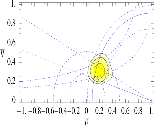
Figure 2:

The agreement in the $\rho-\eta$ plane is certainly significant. At the present state of knowledge, I would summarize it by saying that:

1. no sign of new interactions exists so far in $\Delta B=2$ or $\Delta S=2$;

2. CP violation looks qualitatively or semi-quantitatively as expected in the SM.

The possibility that the SM phase $\delta(CKM)$ be equal to zero, with CP violation accounted for by non SM physics, is, for the first time, rather strongly disfavoured.

3 CP violation as of 2001

3.1 A qualitative change

Although technically correct, to say that CP violation looks as expected in the SM is an understatement. The situation in CP violation has very clearly changed in the past two years. This change can be summarized by making reference to a general effective Lagrangian accounting for CP violation

$${\cal L}^{CP}={\cal L}^{\Delta F=0}+{\cal L}^{\Delta F=1}+{\cal L}^{\Delta F=2}.$$ (4)

On the $\Delta F=0$ piece we still have only limits, a new preliminary one on the electron Electric Dipole Moment, $d_{e}<1.5\cdot 10^{-27}\,\textrm{e cm}$, from Cummings and Regan[8], and on the neutron EDM, $d_{N}<6.3\cdot 10^{-26}\,\textrm{e cm}$. It is more and more true, in my view, that searching for EDMs is a worthy enterprise.

The big change, however, has occurred in the flavour violating pieces of ${\cal L}^{CP}$. We now know for sure that CP violation exists in three different channels, $\Delta S=1$ (from $\epsilon^{\prime}/\epsilon$), $\Delta S=2$ (from $\epsilon$) and $\Delta B=2$ (from $A(B_{d}\rightarrow J/\Psi K_{S})$). Experimental hints existed already before, but these are now established facts. Looking back at the history of CP violation, there is little doubt that this is almost a revolution.

3.2 A general parametrization of CP violation in $\Delta F=2$

It is not difficult to conceive of motivated extensions of the SM which, while accounting for the observations so far, may introduce large deviations from the SM in other observables[9]. In view of this, it makes sense to consider a general parametrization of CP violation in $\Delta F=2$. Concentrating for the moment on the down quark sector, the CP violating effective Lagrangian in the $\Delta F=2$ sector can be written at short distances in the SM as

$${\cal L}^{\Delta F=2}=\sum_{i,j=d,s,b}(V_{td_{i}}V_{td_{j}}^{*})^{2}\,{\cal C}\,(\bar{d}_{i}\gamma_{\mu}(1-\gamma_{5})d_{j})^{2}$$ (5)

where ${\cal C}$ is an overall real coefficient originating from a top loop. Hence ${\cal C}$ is known. A small deviation from the above equation, affecting $\epsilon$, can be easily accounted for and is not relevant to the present discussion.

A general form of ${\cal L}^{\Delta F=2}$ can, on the other hand, be written as

$${\cal L}^{\Delta F=2}=\sum_{\alpha}\sum_{i,j=d,s,b}(V_{td_{i}}V_{td_{j}}^{*})^{2}\,{\cal C}_{ij}^{\alpha}\;O_{ij}^{\alpha}$$ (6)

where $O_{ij}^{\alpha}$ stand for the 4 fermion operators with different Lorentz structures and given flavour indices $i,j$. At the same time the ${\cal C}_{ij}^{\alpha}$ are complex numerical coefficients, normalized for matter of convenience to $(V_{td_{i}}V_{td_{j}}^{*})^{2}$. In principle one would like to measure not only the matrix elements $V_{td_{i}}$ for the different $i$, but also the ${\cal C}_{ij}^{\alpha}$ and eventually compare with the SM form. This task has to be confronted with the experimental information in principle accessible: the determination of the three complex matrix elements

$$\langle K|{\cal L}^{\Delta F}|\bar{K}\rangle,\;\langle B_{d}|{\cal L}^{\Delta F}|\bar{B}_{d}\rangle,\;\langle B_{s}|{\cal L}^{\Delta F}|\bar{B}_{s}\rangle.$$ (7)

To guide this comparison, a useful progression of hypotheses is made, i.e.:

1. Minimal Flavour Violation (MFV)[10]: As in the SM one takes only one 4F-operator, $\alpha=LL$, but one leaves free the real, flavour independent coefficient in front of it. In this case only one new parameter is introduced. As easily seen, neither $A(B_{d}\rightarrow J/\Psi K_{S})$ nor $\frac{\Delta m_{B_{s}}}{\Delta m_{B_{d}}}$ can possibly deviate from their SM values.

2. Generalized MFM[11]: More than one operator can now contribute to ${\cal L}^{\Delta F=2}$, but the ${\cal C}_{ij}^{\alpha}$ are taken to be real and $i,j$-indep. In this case the moduli of the three measurable matrix elements become free. Hence only $A(B_{d}\rightarrow J/\Psi K_{S})$ cannot deviate from the SM value.

This progression of hypotheses can be useful for a practical orientation of the analysis, in case of problems. The real situation, if problems indeed occurred, may be different, however. Deviations from the SM could for example also enter in ${\cal L}^{\Delta F=1}$. I emphasize, quite in general, that there is still ample room for deviations from the SM. To the purpose of making them evident, it will be useful to consider, among the possible tests, a series of possible “null” experiments. In the SM a number of CP asymmetries should either be equal to each other or to zero, as listed below:

$$A(B_{d}\rightarrow J/\Psi K_{S})\; \negthickspace\negthickspace\negthickspace\negthickspace\simeq \;\;A(B_{d}\rightarrow\phi K_{S})$$

$$A(B_{d}\rightarrow J/\Psi K_{S})\; \negthickspace\negthickspace\negthickspace\negthickspace\simeq \;\;A(B_{d}\rightarrow\pi^{0}K_{S})$$

$$A(B^{\pm}\rightarrow\phi K^{\pm}) \negthickspace\negthickspace\negthickspace\negthickspace\simeq \;\;A(B^{\pm}\rightarrow\pi^{\pm}K^{0}) \negthickspace\negthickspace\negthickspace\negthickspace\simeq \;\;0$$

$$A(B_{d}\rightarrow\chi_{s}\gamma) \negthickspace\negthickspace\negthickspace\negthickspace\simeq \;\;0;\;A(B_{s}\rightarrow J/\Psi\phi) \negthickspace\negthickspace\negthickspace\negthickspace\simeq \;\;0$$

The various “$\simeq$” signs do not have equal validity, as it has been discussed in the different cases. These relations can be taken however as a fair first approximation.

For lack of time I do not discuss possible CP violation in the charm quark sector. I only notice that some preliminary indications in charm mixing, reported at previous conferences [12], have not been apparently confirmed here[13].

4 A hidden deeper structure?

Having discussed the present evidence for the empirical adequacy of the FS of the SM, I now turn to the more difficult problem of trying to see if a deeper structure is possibly hidden in the pattern of quark masses and mixings. As I said at the beginning, the difficulty of this problem in no way is an excuse for not trying to attack it.

As well known the problem is hard also because the basic parameters decribing flavour in the SM, the Higgs Yukawa couplings, are not all experimentally accessible, even in principle: while knowledge of the Yukawa matrices $\lambda_{U},\lambda_{D}$ in the quark sector determines the masses and mixings, $m_{U},m_{D}$ and $V_{CKM}$, the reverse is not true. There is qualitative evidence for a hierarchical structure of the type

$$\lambda_{ij}=c_{ij}\,x_{i}\,x_{j} \,\,\text{ \small with}\,\,x_{3}\gg x_{2}\gg x_{1}$$ (8)

$$\!\!\text{\small and }\,c_{ij}=O(1)$$

but to go further is not easy, to say the least. Although several conceptually different approaches have been attempted even in the last two years (Anarchy[14], Extra-dimensions[15], RG flows[16], etc.), time forces me to limit my attention to a more conventional approach, based on the so called “Textures”. I make this choice because the new data discussed above allow for the first time a significant quantitative comparison with the expectations in this framework.

4.1 Textures defined

It may be useful to define as precisely as possible what I mean by “Texture”. There is some flavour basis, at some scale, in which:

1. some of the coefficients $c_{ij}$ vanish;

2. for some (or all the) $c_{ij}$, $|c_{ij}|=|c_{ji}|$;

3. no other precise relation is allowed among the different $c_{ij}$;

4. when the Yukawa matrices for the up and down quarks are diagonalized, the physical masses and angles do not result from accidental cancellations between the various partial contributions involving the $c_{ij}$.

The question that we ask is whether there are relations, exact or approximate, between the physical observables (masses and angles) implied by some texture, as defined above. An important qualification, implicit in 3 and 4, is that these relations should not change in a significant way upon variations of order unity of the $c_{ij}$ (with 1 and 2 above satisfied).

This is a simple-minded approach. Even if one finds such relations, we may not be able to interpret their meaning. I shall come back to this point. It is nevertheless worth a try.

4.2 Texture predictions

In a way or another, many have tried to answer the question raised in the previous subsection. I think that there is in fact a unique set of relations, coherently obtainable following these rules, which are not manifestly inconsistent with the presently known data. They are[17]

$$\left|V_{us}\right|=\left|\sqrt{\frac{m_{d}}{m_{s}}}-e^{i\phi}\sqrt{\frac{m_{u}}{m_{c}}}\right|$$ (9)

$$\left|\frac{V_{ub}}{V_{cb}}\right|=\sqrt{\frac{m_{u}}{m_{c}}}$$ (10)

$$\left|\frac{V_{td}}{V_{ts}}\right|=\sqrt{\frac{m_{d}}{m_{s}}}$$ (11)

where $\phi$ is an arbitrary phase and the various masses are meant to be taken at the same scale, above or at the charm quark mass. The unique texture which produces them[18] is

$$\lambda_{U,\,D}=\lambda_{3,\,3}^{U,\,D}\;\begin{pmatrix}0&\epsilon^{\prime}&0\\[14.22636pt] \epsilon^{\prime}&\epsilon&O(\epsilon)\\[14.22636pt] 0&O(\epsilon)&1\end{pmatrix}$$

with the small parameters $\epsilon^{\prime}\ll\epsilon\ll 1$ being U,D-dependent. The phases of the various entries are not indicated because they are irrelevant. It is important, on the contrary, that $|\lambda_{12}|=|\lambda_{21}|$. Only the size of the 23 and 32 entries matters, as I will show, but not their precise values. In particular they do not need to be symmetric.

By a perturbative diagonalization of these Yukawa matrices the above relations are readily obtained up to corrections of relative order $\epsilon$, i.e. a few $\%$. The explicit diagonalization also shows that the phase $\phi$ in $V_{us}$ is approximately equal to the angle $\alpha$ of the usual unitarity triangle[19].

The texture zeros are crucial. One may in fact wonder how small should the corresponding entries be to maintain the texture relations in an approximate sense. Insisting on relative corrections not exceeding $O(\epsilon)$, it is readily seen that $\lambda_{11}\leq(\epsilon^{\prime})^{2}$, $\lambda_{13}\leq\epsilon\epsilon^{\prime}$ and $\lambda_{31}\leq\epsilon^{\prime}$.

4.3 Comparison with data

To compare the texture relations with data I use[20]

$$Q=\frac{\frac{m_{s}}{m_{d}}}{\sqrt{1-(\frac{m_{u}}{m_{d}})^{2}}}=22.7\pm 0.8,$$ (12)

$$\frac{m_{c}}{m_{s}}=9.3\pm 3.0,$$ (13)

and, but this is a less important entry,

$$\frac{m_{u}}{m_{d}}=0.533\pm 0.043.$$ (14)

The combination $Q$, rather the individual ratios $\frac{m_{s}}{m_{d}}$ and $\frac{m_{u}}{m_{d}}$, is determined without extra assumptions using chiral perturbation theory. The somewhat conservative error on $\frac{m_{c}}{m_{s}}$ is not, in my view, without justification.

With this information on the quark mass ratios, the texture relations allow to determine the Wolfenstein parameters $\rho$ and $\eta$, as shown by the smaller contours in Fig.s 3. As before the contours are at $68$, $95$, $99\%$ C.L. respectively. The difference between Fig. 3a and 3b is that in 3b the coefficients $c_{23}$ and $c_{32}$ are allowed to vary at random and independently from $1/3$ to $3$.

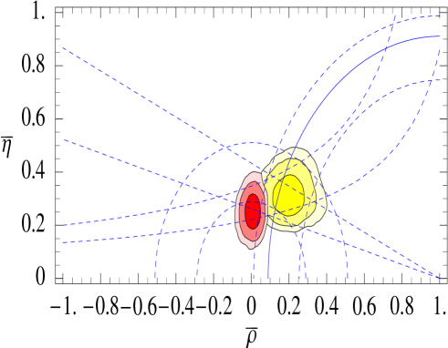
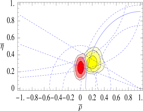
a b

Figure 3:

This determination of $\rho$ and $\eta$ can be compared with experiment, assuming no surprise in genuine FCNCs with respect to SM expectations [22]. To this purpose it is enough to superimpose the contours as obtained from the textures to the fit of the data discussed in Section 2. This comparison is also shown in Fig.s 3.

As anticipated, this comparison starts to be significant. To judge the result, it may be useful to wait for a settlement of the data. Some tension is appearing, however, which would be enhanced if the BELLE result on $A(B_{d}\rightarrow J/\Psi K_{S})$ were included. Two problems seem to emerge: the limit on $\frac{\Delta m_{B_{s}}}{\Delta m_{B_{d}}}$ is too high, as it also seems to be the case for $\left|\frac{V_{ub}}{V_{cb}}\right|$.

In case these difficulties were confirmed, ways out that are proposed involve a modification of the texture[21], like

$$\frac{\lambda_{U,D}}{\lambda_{3,3}^{U,D}}\;\;= \begin{pmatrix}0&\epsilon^{\prime}&0\\ \epsilon^{\prime}&0&O(\epsilon)\\ 0&O(1)&1\end{pmatrix}$$

or $$\begin{pmatrix}0&\epsilon^{\prime}&O(\sqrt{\epsilon}\epsilon\prime)\\ \epsilon^{\prime}&\epsilon&O(\epsilon)\\ O(\sqrt{\epsilon}\epsilon\prime)&O(\epsilon)&1\end{pmatrix}$$ (15)

or the inclusion of some non standard FCNC effects.

In the first case, the loss of predictivity has to be watched. To restore it one may have to include leptons as well. The implication of the second option is that some other deviation in FCNCs should be seen.

4.4 Where does the Texture come from?

If the texture turned out to be successful, we would remain with the problem of interpreting its origin or its meaning. The interpretation I favour calls for the relevance of a $U(2)$ symmetry acting on the first 2 generations as a doublet, supplemented with a straightforward spurion analysis[23], [22]. The spurions may only include a doublet $\phi_{a}$, a triplet $S_{\{a,b\}}$ and an antisymmetric singlet $A_{[a,b]}$. The $U(2)$ symmetry breaking pattern would have to be as follows

$$U(2)\,\stackrel{{\scriptstyle\epsilon:\,\phi_{a},\,S_{\{a,b\}}}}{{\longrightarrow}}\;U(1)\stackrel{{\scriptstyle\epsilon^{\prime}:\,A_{[a,b]}}}{{\longrightarrow}}\emptyset$$

since this would lead to

$$\frac{\lambda_{U,D}}{\lambda_{3,3}^{U,D}}\Rightarrow\begin{pmatrix}0&A_{12}&0\\ -A_{12}&S_{22}&\phi_{2}\\ 0&\phi_{2}&1\end{pmatrix}\Rightarrow\begin{pmatrix}0&\epsilon^{\prime}&0\\ \epsilon^{\prime}&\epsilon&O(\epsilon)\\ 0&O(\epsilon)&1\end{pmatrix}$$

I admit, though, that it may be difficult to prove the relevance of this $U(2)$ symmetry without additional experimental information on flavour physics.

5 Summary and conclusions

The significant flavour measurements performed in the last two years are compatible with the FS of the SM. It is clear, however, that the test is still at a qualitative or only semi-quantitative level. Large deviations from the expectations of the SM in many observables are still possible.

The status of CP violation has seen a qualitative change. $CP$ violation is established in $\Delta S=1$, $\Delta S=2$ and $\Delta B=2$ channels. As a result, the possibility that the CKM phase vanishes, with all of $CP$ violation coming from non SM sources looks, for the first time, clearly disfavoured.

Finally, as a concrete attempt to make sense of the data on quark masses and mixings, a single texture emerges which can be meaningfully compared with the data. It may even have something to do with reality. Quite in general I think that theories of flavour should aim at a comparable level of concreteness.

References

- [1] M. Neubert, these proceedings.
- [2] D. Cassel, CLEO Coll., these proceedings; R. Barate et al, ALEPH Coll., Phys. Lett. B429, 169 (1998); K. Abe et al, BELLE Coll., Phys. Lett. B511, 151 (2001)
- [3] P. Gambino and N. Misiak, hep-ph/0104034, and references therein.
- [4] R. Kessler, these proceedings; L. Iconomidou-Fayard, these proceedings.
- [5] For a review, see A. Buras, talk given at KAON 2001, Pisa, 12 June–17 June, 2001, and references therein.
- [6] J. Dorfan, these proceedings.
- [7] S. Olsen, these proceedings.
- [8] E. Cummings and C. Regan, as presented by E. Hinds, talk given at KAON 2001, Pisa, 12 June–17 June, 2001.
- [9] A. Masiero, M. Piai, A. Romanino and L. Silvestrini, hep-ph/0104101, for an example.
- [10] M. Ciuchini, G. Degrassi, P. Gambino and G. Giudice, Nucl. Phys. B534, 3 (1998); A. Ali and D. London, Phys. Rep. 320, 79 (1999).
- [11] A. Buras, P. Chankowski, J. Rosiek and L. Slawianowska, hep-ph/0107048.
- [12] See I. Bigi, Talk given at the 4th International Conference on B Physics and CP Violation, Ise, Japan, Feb. 19 – 23, 2001, and references therein.
- [13] P. Roudeau, these proceedings.
- [14] L. Hall, H. Murayama, N. Weiner, Phys. Rev. Lett. 84 , 2572 (2000); N. Haba, H. Murayama, Phys. Rev. D63 , 053010 (2001).
- [15] N. Arkani-Hamed, M. Schmaltz, Phys. Rev. D61, 033005 (2000); N. Arkani-Hamed, L. Hall, D. Smith, N. Weiner, Phys. Rev. D61, 116003 (2000).
- [16] A. Nelson and M. Strassler, hep-ph/0104051.
- [17] H. Fritzsch, Nucl. Phys. B155, 189 (1979); P. Ramond, R. Roberts and G. Ross, Nucl. Phys. B406, 19 (1993); L. Hall and A. Rasin, Phys. Lett. B315, 164 (1993).
- [18] L. Hall and A. Rasin, Phys. Lett. B315, 164 (1993);
- [19] R. Barbieri, L. Hall and A. Romanino, Phys. Lett. B401, 47 (1997)
- [20] H. Leutwyler, hep-ph/9602255.
- [21] R. Roberts, A. Romanino, G. Ross, L. Velasco-Sevilla, hep-ph/0104088.
- [22] R. Barbieri, L. Hall and A. Romanino, Nucl. Phys. B551, 93 (1999).
- [23] R. Barbieri, G. Dvali and L. Hall, Phys. Lett. B377, 76 (1996).