Photon Emission from Quark-Gluon Plasma:
Complete Leading Order Results

Abstract

We compute the photon emission rate of an equilibrated, hot QCD plasma at zero chemical potential, to leading order in both $\alpha_{\rm EM}$ and the QCD coupling $g_{\rm s}(T)$. This requires inclusion of near-collinear bremsstrahlung and inelastic pair annihilation contributions, and correct incorporation of Landau-Pomeranchuk-Migdal suppression effects for these processes. Analogous results for a QED plasma are also included.

I Introduction

How brightly does the quark-gluon plasma glow? With the commissioning of RHIC and the future commissioning of the LHC in heavy ion mode, this is becoming an experimental question. It seems appropriate, then, to complete a theoretical analysis of photo-emission from a central heavy ion collision at RHIC or LHC energies.

The goal of this paper is more modest. We will be concerned only with a fully equilibrated quark-gluon plasma, at a temperature high enough that perturbation theory is applicable. In this context we will compute the photo-emission rate to leading order in the strong coupling constant $g_{\rm s}$. By this, we mean the spontaneous emission rate for photons of a given momentum ${\bf k}$, which we will denote as

$$\nu_{\rm e}({\bf k})\equiv(2\pi)^{3}\;{d\Gamma_{\gamma}\over d^{3}{\bf k}}\,.$$ (1)

Our normalization is chosen so that $\Gamma_{\gamma}\equiv\int\nu_{\rm e}({\bf k})\>d^{3}{\bf k}/(2\pi)^{3}$ is the total spontaneous photon emission rate per unit volume.

The evaluation of the photo-emission rate has quite a long history [1, 2, 3, 4, 5, 6, 7, 8], and was thought to have been settled ten years ago when Kapusta et al. [9] and Baier et al. [10] independently computed the diagrams shown in Fig. 1, and obtained the same answer. The result of Refs. [9, 10], written in a slightly more general fashion than given in those papers, is

$$\nu_{\rm e}({\bf k})={\cal A}(k)\left[\,\ln({T}/{m_{\infty}})+{\textstyle{1\over 2}}\ln(2{k}/{T})+C_{2\leftrightarrow 2}(k/T)\,\right],$$ (2)

where $k\equiv|{\bf k}|$ is the energy of the photon. The leading-log coefficient ${\cal A}(k)$ is given by

$${\cal A}(k)=2\,\alpha_{\rm EM}\Big{[}\,d_{\rm F}\sum_{s}q_{s}^{2}\,\Big{]}\;\frac{m_{\infty}^{2}}{k}\>n_{f}(k)\,,$$ (3)

where $n_{f}(k)=[\exp(k/T)+1]^{-1}$ is the Fermi distribution function, and $d_{\rm F}$ is the dimension of the quark representation (so $d_{\rm F}=N_{\rm c}=3$ for QCD). The charge assignment for each quark species $s$ is denoted $q_{s}$, and equals 2/3 for up type and $-1/3$ for down type quarks. The mass $m_{\infty}$ appearing in Eqs. (2) and (3) is the leading-order asymptotic (large momentum) thermal quark mass, given by [11]

$$m_{\infty}^{2}={C_{\rm F}\,g_{\rm s}^{2}\,T^{2}\over 4}\,,$$ (4)

with $C_{\rm F}$ the quadratic Casimir of the quark representation. For the fundamental representation of SU($N_{\rm c}$), $C_{\rm F}=(N_{\rm c}^{2}{-}1)/(2N_{\rm c})$; for QCD specifically, $C_{\rm F}=4/3$ and $m_{\infty}^{2}={g_{\rm s}^{2}\,T^{2}}/{3}$. Hence, for two-flavor QCD, the leading-log coefficient is explicitly

$${\cal A}(k)={40\,\pi T^{2}\over 9}\,\alpha_{\rm EM}\,\alpha_{\rm s}\,{n_{f}(k)\over k}\,.$$ (5)

The strong coupling $g_{\rm s}$ (and $\alpha_{\rm s}\equiv g_{\rm s}^{2}/4\pi$) should always be understood as defined at a scale of order of the temperature.

The final term $C_{2\leftrightarrow 2}(k/T)$ in expression (2) is a function of $k/T$ with a finite limit as $k/T\to\infty$. The papers [9, 10] compute $C_{2\leftrightarrow 2}(k/T)$ only in this limit, and find

$$\lim_{k/T\rightarrow\infty}C_{2\leftrightarrow 2}(k/T)=-\frac{1}{4}-\frac{\gamma_{\rm E}}{2}+\frac{2\ln(2)}{3}+\frac{\zeta^{\prime}(2)}{2\zeta(2)}\simeq-0.3614902\,.$$ (6)

We have also verified this result.

FIG. 1.: Two-to-two particle processes which generate the leading logarithmic contribution to the photo-production rate, and were originally believed to give the complete leading order contribution. Time may be viewed as running from left to right.

FIG. 2.: Inelastic processes which, because of near-collinear singularities, contribute at the same order as the two-to-two particle processes. The diagrams on the left represent bremsstrahlung, and those on the right are inelastic pair annihilation. Again, time may be viewed as running from left to right.

However, as recently demonstrated by Aurenche et al. [12, 13, 14], the result (2) is incomplete. The bremsstrahlung and inelastic pair annihilation processes shown in Fig. 2 contain collinear enhancements which cause them to contribute at the same parametric order in coupling, $O(\alpha_{\rm EM}\,\alpha_{\rm s})$, as the two-to-two processes of Fig. 1, even for large photon energies $k\gg T$. But the calculation of these processes presented in [12] is also incomplete, as it fails to incorporate an $O(1)$ suppression of these processes due to multiple scattering during the photon emission process, which limits the coherence length of the emitted radiation. This is known as the Landau-Pomeranchuk-Migdal (LPM) effect [16, 17, 18]. The presence of LPM suppression was pointed out in later work by Aurenche et al. [13, 14], which discussed the physics involved but did not attempt to make a complete calculation.

This paper presents a full calculation of the photon emission rate at leading order in $g_{\rm s}$. We evaluate the non-logarithmic two-to-two contribution $C_{2\leftrightarrow 2}(k/T)$ for general $k/T$. We also compute the rate of photo-production by bremsstrahlung and inelastic pair annihilation, fully including the LPM effect. This requires solving a non-trivial integral equation to determine this rate. We derived this integral equation in Ref. [19]; it is related to one written down over 45 years ago by Migdal [17, 18] for studying electromagnetic energy loss of a relativistic particle traversing matter. Related work in the QCD context may be found in Refs. [20, 21, 22, 23, 24, 25]. Other discussions of the LPM effect for electromagnetic interactions in ordinary matter include Refs. [27, 28, 29]. The current paper is a sequel to our earlier work [19], but it should be fairly self-contained.

The outline of the remainder of this paper is as follows. In Sec. II, we briefly review our previous work [19] showing why the processes considered here (and no others) contribute to the leading order emission rate, and deriving an integral equation whose solution determines the bremsstrahlung and inelastic pair annihilation contributions to the emission rate, fully including the LPM effect. Sec. III discusses, qualitatively, the relative importance of the LPM effect in different kinematic regimes. The numerical solution of the integral equation determining the LPM contributions to the emission rate is presented in Sec. IV. This section is the meat of the paper. Sec. V contains the evaluation of $C_{2\leftrightarrow 2}(k/T)$ for arbitrary photon energy $k\gg g_{\rm s}T$. (If this condition is violated, then thermal corrections to the dispersion relations for incoming or outgoing particles can no longer be neglected in these $2\leftrightarrow 2$ processes.) Our results are combined in Sec. VI, which is followed by a brief conclusion.

For the convenience of readers interested in just the bottom line, we summarize our results here. The complete leading-order photon emission rate may be written as

$$\nu_{\rm e}({\bf k}) = {\cal A}(k)\,\Bigl{[}\,\ln\left({T}/{m_{\infty}}\right)+C_{\rm tot}(k/T)\,\Bigr{]}\,,$$ (7)

with

$$C_{\rm tot}(k/T) \equiv {\textstyle{1\over 2}}\ln\left({2k}/{T}\right)+C_{2\leftrightarrow 2}(k/T)+C_{\rm brem}(k/T)+C_{\rm annih}(k/T)\,,$$ (8)

and the coefficient ${\cal A}(k)$ given in Eq. (3). The function $C_{\rm tot}(k/T)$ is the total “constant under the log”; it is a non-trivial function of $k/T$ but it is independent of the strong coupling $g_{\rm s}$, whereas $\ln(T/m_{\infty})\sim\ln(1/g_{\rm s})$ since $m_{\infty}=O(g_{\rm s}\,T)$. Corrections to Eq. (7) are suppressed by one or more powers of $g_{\rm s}$.

The functions $C_{2\leftrightarrow 2}(k/T)$, $C_{\rm brem}(k/T)$, and $C_{\rm annih}(k/T)$ all involve multidimensional integrals (or integral equations) which cannot be evaluated analytically but may be computed numerically. Individual plots of these functions, as well as their sum, are shown in section VI. Our numerical results for QCD plasmas are reproduced quite accurately by the approximate, phenomenological fits

$$C_{2\leftrightarrow 2}(x) \simeq 0.041\,x^{-1}-0.3615+1.01\,e^{-1.35\,x}\,,$$ (9)

and

$$C_{\rm brem}(x)+C_{\rm annih}(x) \simeq \sqrt{1{+}{\textstyle{1\over 6}}N_{\rm f}}\left[\frac{0.548\,\log(12.28+1/x)}{x^{3/2}}+\frac{0.133\,x}{\sqrt{1+x/16.27}}\right],$$ (10)

where $N_{\rm f}$ is the number of quark flavors. The approximation (9) to the function $C_{2\leftrightarrow 2}(x)$ (which crosses zero) is accurate to within an absolute error of 0.02 over the range $0.2\leq k/T\leq 50$, but this form fails to be a good approximation at smaller $k/T$; $C_{2\leftrightarrow 2}(x)$ has a finite small $x$ limit, rather than growing as $1/x$. As discussed in section III, the form (10) for the near-collinear contributions builds in the right parametric large and small $k$ asymptotic behavior, up to logs, and is accurate to within a 3% relative error over the range $0.2\leq k/T\leq 50$ for $N_{\rm f}$ from 2 to 6.

Consider, for the sake of discussion, a value of $\alpha_{\rm s}=0.2$ which corresponds to $\ln(T/m_{\infty})=0.09$. In this case, it turns out that the old results of Baier et al. [10] and Kapusta et al. [9], which neglect near-collinear bremsstrahlung and inelastic pair annihilation, are within a factor of two of the correct leading-order rate for photon momenta in the range $2.5\leq k/T\leq 10$. Bremsstrahlung becomes the most important process for energies below this range, and inelastic pair annihilation makes a large relative contribution to the rate above this range (where the total rate is small because of exponentially falling population functions). The LPM effect suppresses both bremsstrahlung and pair annihilation processes, but the suppression is not severe (35% or less) except for soft bremsstrahlung with $k\leq 2T$, or very hard pair annihilation with $k\gg 10T$, where the LPM suppression is significant. For parametrically small photon energy $k\ll T$ (but with $k\gg eT$ and $k\gg g_{\rm s}^{4}T\ln g_{\rm s}^{-1}$), the LPM effect changes the parametric behavior of the emission rate. One finds,

$${d\Gamma_{\gamma}}\propto k^{-1/2}\,dk\,,$$ (11)

[ignoring $\log(T/k)$ factors], rather than $k^{-1}\,dk$ which is the result if one ignores the LPM effect. Therefore some results in the literature [12, 26] concerning soft, on-shell photo-emission from the quark gluon plasma, ignoring the LPM effect, are wrong parametrically. Similarly, for extremely hard photon emission, the rate behaves as $k^{3/2}\,e^{-k/T}dk$, rather than $k^{2}\,e^{-k/T}dk$ as one would obtain by neglecting the LPM effect. For more detailed results see the figures in Sec. VI.

II Bremsstrahlung and inelastic pair annihilation

FIG. 3.: Typical ladder diagram contributing to the electromagnetic current-current correlator. All such ladder diagrams must be summed to determine the leading-order bremsstrahlung and inelastic pair annihilation rates. Resummation of self-energy insertions on all propagators is implied.

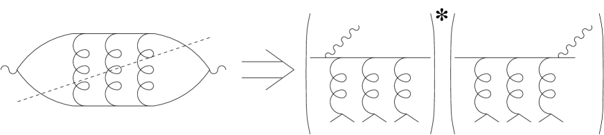
FIG. 4.: Cut ladder diagram with $N$ gluon “rungs” may be interpreted as the interference between amplitudes for photon emission before and after $N$ scattering events.

The photo-emission rate is related to the imaginary part of the electromagnetic current-current correlator. We show in [19] that a correct treatment of the near-collinear bremsstrahlung and inelastic pair annihilation processes which contribute to the leading-order emission rate requires a summation of all ladder graphs of the form shown in Fig. 3. (Self-energy insertions on all propagators, including the leading order imaginary parts, are implicitly resummed.) As indicated in Fig. 4, these diagrams can be interpreted as generating various contributions to the squares of scattering amplitudes. It is necessary to sum all ladders because there can be interference between emission at one scattering and at subsequent scattering events. This is the basic origin of the LPM effect.

The total photon emission rate is given by an integral over all particle momenta of the emission rate for that particle momentum. Factoring out the same coefficient ${\cal A}(k)$ which appears in the leading logarithmic result (2), we find that the contribution of bremsstrahlung and inelastic pair annihilation processes to the leading-order emission rate is [19]

$$\nu_{\rm e}^{\scriptscriptstyle\rm LPM}({\bf k}) = {\cal A}(k)\!\int_{-\infty}^{\infty}\!\!d{p_{\parallel}}\left[\frac{{p_{\parallel}}^{2}+({p_{\parallel}}{+}k)^{2}}{4{p_{\parallel}}^{2}\,({p_{\parallel}}{+}k)^{2}}\right]\!\frac{n_{f}(k{+}{p_{\parallel}})\,[1{-}n_{f}({p_{\parallel}})]}{m_{\infty}^{2}\,n_{f}(k)}\!\int\!\frac{d^{2}{\bf p}_{\perp}}{(2\pi)^{2}}\,{\rm Re}\left\{2{\bf p}_{\perp}\!\cdot{\bf f}({\bf p}_{\perp},{p_{\parallel}},k)\right\}\!.$$ (12)

Here ${p_{\parallel}}$ and ${\bf p}_{\perp}$ are the components of the momentum ${\bf p}$ parallel or perpendicular to the photon direction, respectively. The contribution from the integration region $-k<{p_{\parallel}}<0$, in which ${p_{\parallel}}$ and $({p_{\parallel}}{+}k)$ have opposite sign and $1{-}n_{f}({p_{\parallel}})=n_{f}(|{p_{\parallel}}|)$, should be interpreted as inelastic pair annihilation, while the contributions from ${p_{\parallel}}>0$ or ${p_{\parallel}}<-k$ represent bremsstrahlung off a particle of energy ${p_{\parallel}}{+}k$ (when ${p_{\parallel}}>0$) or an anti-particle of energy $-{p_{\parallel}}$ (for ${p_{\parallel}}<-k$).

The final term ${\rm Re}\{2{\bf p}_{\perp}\cdot{\bf f}({\bf p}_{\perp},{p_{\parallel}},k)\}$ is proportional to the amplitude squared for a particle of momentum ${\bf p}{+}{\bf k}$ to emit a photon of momentum ${\bf k}$, and is the non-trivial part of the calculation. The function ${\bf f}({\bf p}_{\perp},{p_{\parallel}},k)$ is the solution to an integral equation, derived in [19], which accounts for the partial coherence between multiple scattering events. This integral equation is

$$2{\bf p}_{\perp} = i\,\delta E({\bf p}_{\perp})\>{\bf f}({\bf p}_{\perp})+\int{d^{2}{\bf q}_{\perp}\over(2\pi)^{2}}\;{\cal C}({\bf q}_{\perp})\,\Big{[}{\bf f}({\bf p}_{\perp})-{\bf f}({\bf p}_{\perp}{+}{\bf q}_{\perp})\Big{]}\,,$$ (14)

where the dependence of ${\bf f}({\bf p}_{\perp},{p_{\parallel}},k)$ (as well as $\delta E$) on ${p_{\parallel}}$ and $k$ has been suppressed for notational convenience. The collision kernel ${\cal C}({\bf q}_{\perp})$ is given by

$${\cal C}({\bf q}_{\perp})\equiv\frac{m_{\rm D}^{2}\,m_{\infty}^{2}}{T^{2}}\int{dq_{\parallel}\,dq^{0}}\>\delta(q_{\parallel}{-}q^{0})\,\frac{T}{q}\left\{\frac{2}{\left|q^{2}-\Pi_{\rm L}(q^{0},q)\right|^{2}}+\frac{[1-(q^{0}/q)^{2}]^{2}}{\left|(q^{0})^{2}-q^{2}-\Pi_{\rm T}(q^{0},q)\right|^{2}}\right\},$$ (15)

where $q\equiv|{\bf q}|=[{\bf q}_{\perp}^{2}+{q_{\parallel}}^{2}]^{1/2}$, $m_{\rm D}$ is the (leading order) Debye mass, and $\Pi_{\rm L}(q^{0},q)$ and $\Pi_{\rm T}(q^{0},q)$ are the standard hard thermal loop longitudinal and transverse gluon self-energies [30], respectively; their explicit form is given in Section IV. In the first term on the right-hand side of Eq. (14), $\delta E$ denotes the energy difference, on shell, between the two relevant states of the system, in the limit where ${p_{\parallel}}$ is large compared to $|{\bf p}_{\perp}|$ and $m_{\infty}$. For bremsstrahlung, this is the energy difference between a quark of momentum ${\bf p}$ plus a photon of momentum ${\bf k}$, and a quark of momentum ${\bf p}{+}{\bf k}$, which explicitly is

$$\delta E({\bf p}_{\perp},{p_{\parallel}},k) = \left({p_{\parallel}}+{{\bf p}_{\perp}^{2}+m_{\infty}^{2}\over 2{p_{\parallel}}}\right)+\left(k+{m_{\gamma}^{2}\over 2k}\right)-\left({p_{\parallel}}+k+{{\bf p}_{\perp}^{2}+m_{\infty}^{2}\over 2({p_{\parallel}}{+}k)}\right)$$ (16)

$$= \frac{k}{2{p_{\parallel}}(k{+}{p_{\parallel}})}\left[{\bf p}_{\perp}^{2}+m_{\infty}^{2}\right]+\frac{m_{\gamma}^{2}}{2k}\,.$$ (17)

For pair annihilation, $\delta E$ is the difference between a quark plus anti-quark with momenta $-{\bf p}$ and ${\bf p}{+}{\bf k}$, and a photon of momentum ${\bf k}$; this gives exactly the same result (17) given our convention about the sign of ${p_{\parallel}}$. This energy difference generates a phase difference between the amplitudes in Fig. 4, which is manifested as an imaginary term in Eq. (14). This phase difference will eliminate coherence in the emitted radiation beyond a time scale of order $1/\delta E$, which is often referred to as the formation time of the photon. The $m_{\gamma}^{2}$ contribution to $\delta E$ accounts for plasma induced dispersion in the photon propagation; $m_{\gamma}$ is the asymptotic thermal photon mass, whose square is half the electromagnetic Debye mass squared of the plasma,

$$m_{\gamma}^{2}={\textstyle{1\over 2}}\,m_{{\rm D},\gamma}^{2}={1\over 6}\,\Big{[}\,d_{\rm F}\sum_{s}q_{s}^{2}\,\Big{]}\,e^{2}\,T^{2}\,.$$ (18)

Since we assume $\alpha_{\rm EM}\ll\alpha_{\rm s}$, we may neglect this electromagnetic dispersion correction when considering photo-emission from a quark-gluon plasma; but when we consider the emissivity of an electromagnetic plasma, which we will also compute, retaining this term will be essential.

Note that the collision kernel (15) is rotationally invariant (in the transverse plane). Consequently, the solution to the integral equation (14) must equal ${\bf p}_{\perp}$ times some scalar function of ${\bf p}_{\perp}^{2}$,

$${\bf f}({\bf p}_{\perp})={\bf p}_{\perp}\,\chi(p_{\perp}^{2})\,.$$ (19)

Hence, although written as a vector equation, the integral equation (14) is trivially reducible to a scalar integral equation. For later convenience, also note that this integral equation may be written more abstractly as $2{\bf p}_{\perp}=[i\,\delta E+\hat{\cal C}\,]\,{\bf f}$, if one defines $\hat{\cal C}$ as a linear operator acting on functions of ${\bf p}_{\perp}$, whose explicit form is given by the second term in Eq. (14). Further discussion of equation (14), and its derivation, may be found in Ref. [19].

III LPM effect: Rough Estimates

Before solving equation (14) numerically, it is useful to examine in what kinematic regimes the LPM effect will be important and to estimate how large its effect can be. Neglecting the LPM effect altogether means ignoring any interference between successive scattering processes. This corresponds to solving Eq. (14) under the assumption that $\delta E$ is much greater than the collision term which follows it. At leading order in this “approximation,” ${\bf f}({\bf p}_{\perp})$ is then pure imaginary,

$${\rm Im}\,{\bf f}({\bf p}_{\perp})\Big{|}_{\rm no\;LPM}=-\frac{2{\bf p}_{\perp}}{\delta E({\bf p}_{\perp})}\,.$$ (20)

The next order arises from substituting this result into the collision term, thereby determining the leading real part of ${\bf f}$ in this approximation,

$${\rm Re}\,{\bf f}({\bf p}_{\perp})\Big{|}_{\rm no\;LPM}=\frac{1}{\delta E({\bf p}_{\perp})}\int{d^{2}{\bf q}_{\perp}\over(2\pi)^{2}}\;{\cal C}({\bf q}_{\perp})\left[\frac{2{\bf p}_{\perp}}{\delta E({\bf p}_{\perp})}-\frac{2({\bf p}_{\perp}{+}{\bf q}_{\perp})}{\delta E({\bf p}_{\perp}{+}{\bf q}_{\perp})}\right]\,.$$ (21)

Inserting this form for ${\rm Re}\,{\bf f}({\bf p}_{\perp})$ into Eq. (LABEL:eq:outer_int) reproduces the results of Aurenche et al. [12] (except for the overall factor of 4 error made there [15]). Given the form (17) of $\delta E$, and neglecting $m_{\gamma}^{2}$, one may see without performing any calculation that ${\rm Re}\,{\bf f}({\bf p}_{\perp})|_{\rm no\;LPM}$ will be a ${p_{\parallel}}$ and $k$ independent function times ${p_{\parallel}}^{2}({p_{\parallel}}{+}k)^{2}/k^{2}$. Therefore, in this approximation, the photon spectrum will look like

$$\nu_{\rm e}({\bf k})\Big{|}_{\rm no\;LPM}\propto{\cal A}(k)\int_{-k/2}^{\infty}d{p_{\parallel}}\left[\frac{{p_{\parallel}}^{2}+({p_{\parallel}}{+}k)^{2}}{k^{2}\,T}\right]\frac{n_{f}(k{+}{p_{\parallel}})\,[1{-}n_{f}({p_{\parallel}})]}{n_{f}(k)}\,,$$ (22)

with a $k$-independent constant of proportionality. For soft photons ($k\ll T$) the dominant contribution comes from ${p_{\parallel}}\sim T$, and the result, ignoring the LPM effect, grows as $T^{2}/k^{2}$ relative to the emission rate due to only $2\leftrightarrow 2$ processes. At large $k\gg T$ the dominant contribution comes from the whole range $-k/2<{p_{\parallel}}<0$ over which the population function terms are approximately unity. This yields a result (again, ignoring the LPM effect) which grows as $k/T$ relative to the $2\leftrightarrow 2$ emission rate. Therefore, ignoring the LPM effect, we find that bremsstrahlung dominates the emission rate for $k\ll T$, while inelastic pair annihilation dominates the rate for $k\gg T$.

We must now consider whether, for any range of $k$, it is actually permissible to neglect the LPM effect. Using the form (17) of $\delta E$, one may easily see that if $kT/|{p_{\parallel}}\,({p_{\parallel}}{+}k)|$ is sufficiently large then $|\delta E|$ will also be large for all ${\bf p}_{\perp}$ and an expansion based on $|\delta E|\gg\hat{\cal C}$ will be valid for all ${\bf p}_{\perp}$. However, in this regime, ${\rm Re}\,{\bf f}$ is always small, and so is the photo-emission rate. In both cases where we have just found a large photo-emission rate (ignoring LPM suppression), the quantity $kT/[{p_{\parallel}}\,({p_{\parallel}}{+}k)]$ is small, and hence the inequality $\delta E\gg\hat{\cal C}$ only holds for large ${\bf p}_{\perp}$. Therefore, the estimates we have just made are too optimistic, and there will be substantial LPM suppression in exactly those regimes where the inelastic rate is dominant. To estimate how large the suppression is, we may solve for ${\bf f}({\bf p}_{\perp})$ at large ${\bf p}_{\perp}$, where the large $\delta E$ approximation is valid, and determine where the approximation breaks down. At large ${\bf p}_{\perp}$, we have

$$\left.{\rm Im}\,{\bf f}({\bf p}_{\perp})\right|_{\rm asymptotic}=-\frac{2{\bf p}_{\perp}}{\delta E({\bf p}_{\perp})}\simeq-\left[\frac{2{p_{\parallel}}\,({p_{\parallel}}{+}k)}{k}\right]\frac{2{\bf p}_{\perp}}{{\bf p}_{\perp}^{2}}\,,$$ (23)

and

$$\left.{\rm Re}\,{\bf f}({\bf p}_{\perp})\right|_{\rm asymptotic} = \frac{-1}{\delta E({\bf p}_{\perp})}\;\hat{\cal C}\>{\rm Im}\,{\bf f}|_{\rm asymptotic}$$ (24)

$$\simeq \left[\frac{2{p_{\parallel}}\,({p_{\parallel}}{+}k)}{k}\right]^{2}\frac{1}{{\bf p}_{\perp}^{2}}\int{d^{2}{\bf q}_{\perp}\over(2\pi)^{2}}\;{\cal C}({\bf q}_{\perp})\left[\frac{2{\bf p}_{\perp}}{{\bf p}_{\perp}^{2}}-\frac{2({\bf p}_{\perp}{+}{\bf q}_{\perp})}{({\bf p}_{\perp}{+}{\bf q}_{\perp})^{2}}\right].$$ (25)

This integral may be evaluated in closed form. Since the kernel ${\cal C}({\bf q}_{\perp})$ is rotationally invariant, the integral in Eq. (25) may be rewritten as

$$\int_{0}^{\infty}{d|{\bf q}_{\perp}|\over 2\pi}\>|{\bf q}_{\perp}|\>{\cal C}(|{\bf q}_{\perp}|)\left[{2{\bf p}_{\perp}\over{\bf p}_{\perp}^{2}}-\left<{2{\bf p}_{\perp}\over{\bf p}_{\perp}^{2}}\right>_{\!q_{\perp}}\right],$$ (26)

where $\left<g({\bf p}_{\perp})\right>_{q_{\perp}}$ denotes the average of a function $g$ over the circle of radius $q_{\perp}\equiv|{\bf q}_{\perp}|$ centered at ${\bf p}_{\perp}$. Next, note that (both components of) ${\bf p}_{\perp}/{\bf p}_{\perp}^{2}$ are harmonic functions (away from ${\bf p}_{\perp}=0$), and recall that the average of a harmonic function around a circle equals the value of the function at the center of the circle, provided no singularities are enclosed. Consequently, the integrand of Eq. (26) vanishes for $|{\bf q}_{\perp}|<|{\bf p}_{\perp}|$. For $|{\bf q}_{\perp}|>|{\bf p}_{\perp}|$, elementary complex analysis shows that $\left<{\bf p}_{\perp}/{\bf p}_{\perp}^{2}\right>_{q_{\perp}}$ vanishes. Therefore,

$$\left.{\rm Re}\,{\bf f}({\bf p}_{\perp})\right|_{\rm asymptotic}={1\over\pi}\left[\frac{2{p_{\parallel}}\,({p_{\parallel}}{+}k)}{k}\right]^{2}\frac{{\bf p}_{\perp}}{|{\bf p}_{\perp}|^{4}}\int_{|{\bf p}_{\perp}|}^{\infty}{\cal C}(|{\bf q}_{\perp}|)\,|{\bf q}_{\perp}|\,{d|{\bf q}_{\perp}|}\,.$$ (27)

Since ${\bf p}_{\perp}$ has been assumed to be asymptotically large, and $|{\bf q}_{\perp}|>|{\bf p}_{\perp}|$, one may completely neglect the self-energy corrections in the explicit form (15) of ${\cal C}({\bf q}_{\perp})$. The resulting integral is then straightforward, leading to

$${\rm Re}\,{\bf f}({\bf p}_{\perp})|_{\rm asymptotic}=\left[\frac{2{p_{\parallel}}({p_{\parallel}}{+}k)}{k}\right]^{2}{m_{\rm D}^{2}\,m_{\infty}^{2}\over\pi\,T}\,\frac{2{\bf p}_{\perp}}{|{\bf p}_{\perp}|^{6}}\,.$$ (28)

These large ${\bf p}_{\perp}$ asymptotic forms are valid when $\delta E\gg\hat{\cal C}$, or equivalently when ${\rm Re}\,{\bf f}({\bf p}_{\perp})|_{\rm asymptotic}\ll{\rm Im}\,{\bf f}({\bf p}_{\perp})|_{\rm asymptotic}$. The expansion will have broken down when the real and imaginary parts become comparable. This occurs for

$${\bf p}_{\perp}^{2}\sim\left.{\bf p}_{\perp}^{2}\right|_{\rm crossover}\equiv{m_{\rm D}\,m_{\infty}}\,\sqrt{\frac{{p_{\parallel}}\,({p_{\parallel}}{+}k)}{kT}}\,.$$ (29)

Below this crossover point, ${\rm Re}\,{\bf f}({\bf p}_{\perp})$ will be smaller than the asymptotic estimate. The region ${\bf p}_{\perp}\sim{\bf p}_{\perp}|_{\rm crossover}$ will, in fact, provide the dominant contribution to the final $d^{2}{\bf p}_{\perp}$ integral in the rate (LABEL:eq:outer_int). Hence the size of this integral [ignoring factors of $\ln(k/T)$] may be estimated as

$$\int_{{\bf p}_{\perp}^{2}|_{\rm crossover}}^{\infty}d(p_{\perp}^{2})\>{\rm Re}\,{\bf f}|_{\rm asymptotic}\cdot{\bf p}_{\perp} \sim \left[\frac{{p_{\parallel}}\,({p_{\parallel}}{+}k)}{k}\right]^{2}\frac{m_{\rm D}^{2}\,m_{\infty}^{2}}{T\,{\bf p}_{\perp}^{2}|_{\rm crossover}}$$ (30)

$$\sim \left[\frac{{p_{\parallel}}({p_{\parallel}}{+}k)}{kT}\right]^{3/2}{m_{\rm D}\,m_{\infty}\,T}\,.$$ (31)

Using this result, we find that, for bremsstrahlung, the small $k$ emission rate grows, relative to the $2\leftrightarrow 2$ rate, only as $(T/k)^{3/2}$, not $(T/k)^{2}$ as was found ignoring the LPM effect. Similarly, for large $k$ the inelastic pair annihilation rate grows, relative to the $2\leftrightarrow 2$ rate, only as $(k/T)^{1/2}$, not $(k/T)$ as was found when ignoring LPM. The dependence on $m_{\rm D}$ is also simple; relative to the $2\leftrightarrow 2$ rate, the inelastic contribution grows linearly in the Debye mass $m_{\rm D}$. Therefore, inelastic processes become relatively more important as we increase the number of species in the plasma (which increases $m_{\rm D}$), but only as the square root of the number of species.

IV Solving the integral equation

In order to solve the integral equation (14) which determines ${\bf f}({\bf p}_{\perp})$, we will use an adaptation of the variational approach we previously exploited in [31, 32]. But first, it will be convenient to scale out the dimensionful parameters from Eq. (14). To do so, we define dimensionless transverse momenta,

$$\tilde{\bf p}_{\perp}\equiv\frac{{\bf p}_{\perp}}{m_{\rm D}}\,,\quad\tilde{{\bf q}}\equiv\frac{{\bf q}}{m_{\rm D}}\,,\quad$$ (32)

and correspondingly define

$${\widetilde{\delta E}\rule{0.0pt}{9.90276pt}}(\tilde{\bf p}_{\perp})\equiv\frac{T}{m_{\rm D}^{2}}\,\delta E({\bf p}_{\perp})\,,\qquad\tilde{\bf f}(\tilde{\bf p}_{\perp})\equiv\frac{m_{\rm D}}{T}\,{\bf f}({\bf p}_{\perp})\,.$$ (33)

It will also be convenient to define the dimensionless ratio of thermal masses

$$\kappa\equiv\frac{m_{\infty}^{2}}{m_{\rm D}^{2}}=\frac{3C_{\rm F}}{4(T_{\rm A}+N_{\rm f}\,T_{\rm F})}=\left\{\begin{array}[]{ll}3/(4N_{\rm f})\,,&{\rm QED}\,;\\ 2/(6+N_{\rm f})\,,&{\rm QCD}\,.\\ \end{array}\right.$$ (34)

Here $T_{\rm A}$ and $T_{\rm F}$ are the trace normalizations of the adjoint and quark representations, respectively. For QCD, $T_{\rm A}=N_{\rm c}=3$ and $T_{\rm F}=1/2$, while for QED, $T_{\rm A}=0$, and $T_{\rm F}=1$.

Substituting these dimensionless variables into Eq. (LABEL:eq:outer_int), and noting that the argument of the ${p_{\parallel}}$ integral is invariant under ${p_{\parallel}}\rightarrow-k-{p_{\parallel}}$, that equation becomes

$$\nu_{\rm e}^{\scriptscriptstyle\rm LPM}({\bf k}) = {{\cal A}(k)\,T\over\kappa}\int_{-k/2}^{\infty}d{p_{\parallel}}\left[\frac{{p_{\parallel}}^{2}+({p_{\parallel}}{+}k)^{2}}{2{p_{\parallel}}^{2}\,({p_{\parallel}}{+}k)^{2}}\right]\frac{n_{f}(k{+}{p_{\parallel}})\,[1{-}n_{f}({p_{\parallel}})]}{n_{f}(k)}\>\Big{(}2\tilde{\bf p}_{\perp}\,,\,{\rm Re}\,\tilde{\bf f}\Big{)}\,,$$ (35)

where we have introduced a natural inner product on the space of (vector valued) functions of transverse momentum,

$$\Big{(}{\bf f}_{1}\,,\,{\bf f}_{2}\Big{)}\equiv\int\frac{d^{2}\tilde{\bf p}_{\perp}}{(2\pi)^{2}}\;{\bf f}_{1}(\tilde{\bf p}_{\perp})\cdot{\bf f}_{2}(\tilde{\bf p}_{\perp})\,.$$ (36)

Once again, the contribution from ${p_{\parallel}}<0$ is inelastic pair annihilation, while the contribution from ${p_{\parallel}}>0$ is bremsstrahlung. The dimensionless form of the integral equation for $\tilde{\bf f}$ is now

$$2\tilde{\bf p}_{\perp}=\left[i{\widetilde{\delta E}\rule{0.0pt}{9.90276pt}}+\tilde{\cal C}\,\right]\tilde{\bf f}\,,$$ (37)

where

$${\widetilde{\delta E}\rule{0.0pt}{9.90276pt}}=\cases{\displaystyle\frac{kT}{2{p_{\parallel}}\,(k{+}{p_{\parallel}})}\left[\tilde{\bf p}_{\perp}^{2}+\kappa\right],&QCD;\cr\displaystyle\frac{kT}{2{p_{\parallel}}\,(k{+}{p_{\parallel}})}\left[\tilde{\bf p}_{\perp}^{2}+\kappa\right]+{T\over 4k}\,,&QED,}$$ (38)

and

$$(\tilde{\cal C}\,\tilde{\bf f})(\tilde{\bf p}_{\perp})=\int\frac{d^{2}\tilde{\bf q}_{\perp}}{(2\pi)^{2}}\;\tilde{\cal C}(\tilde{\bf q}_{\perp})\Big{[}\tilde{\bf f}(\tilde{\bf p}_{\perp})-\tilde{\bf f}(\tilde{\bf p}_{\perp}{+}\tilde{\bf q}_{\perp})\Big{]}\,,$$ (39)

with

$$\tilde{\cal C}(\tilde{\bf q}_{\perp})\equiv\kappa\int d\tilde{q_{\parallel}}\>d\tilde{q}^{0}\;\delta(\tilde{q_{\parallel}}{-}\tilde{q}^{0})\,\frac{1}{\tilde{q}}\left\{\frac{2}{\left|\tilde{q}^{2}-\tilde{\Pi}_{\rm L}(\tilde{q}^{0},\tilde{q})\right|^{2}}+\frac{[1-(\tilde{q}^{0}/\tilde{q})^{2}]^{2}}{\left|(\tilde{q}^{0})^{2}-\tilde{q}^{2}-\tilde{\Pi}_{\rm T}(\tilde{q}^{0},\tilde{q})\right|^{2}}\right\}.$$ (40)

Here $\tilde{q_{\parallel}}\equiv{q_{\parallel}}/m_{\rm D}$, $\tilde{q}^{0}\equiv q^{0}/m_{\rm D}$, and $\tilde{q}\equiv\sqrt{\tilde{\bf q}_{\perp}^{2}+\tilde{q}_{\parallel}^{2}}$. The explicit forms of the thermal gauge field self energies are [30]

$$\tilde{\Pi}_{\rm L}(\tilde{q}^{0},\tilde{q}) = -1+\frac{\tilde{q}^{0}}{2\tilde{q}}\left[\ln\left(\frac{\tilde{q}{+}\tilde{q}^{0}}{\tilde{q}{-}\tilde{q}^{0}}\right)-i\pi\right],$$ (41)

$$\tilde{\Pi}_{\rm T}(\tilde{q}^{0},\tilde{q}) = \frac{(\tilde{q}^{0})^{2}}{2\tilde{q}^{2}}+\left[\tilde{q}^{2}-(\tilde{q}^{0})^{2}\right]\frac{\tilde{q}^{0}}{4\tilde{q}^{3}}\left[\ln\left(\frac{\tilde{q}{+}\tilde{q}^{0}}{\tilde{q}{-}\tilde{q}^{0}}\right)-i\pi\right].$$ (42)

These forms are valid for $\tilde{q}>|\tilde{q}^{0}|$, which is enforced by the delta function in (40) which identifies $\tilde{q}^{0}$ with $\tilde{q}_{\parallel}$. Both ${\widetilde{\delta E}\rule{0.0pt}{9.90276pt}}$ and $\tilde{\cal C}$ should be viewed as linear operators on the vector space of functions of transverse momentum. Both operators are Hermitian — in fact, real and symmetric — under the inner product (36).

A Variational approach

We are unable to find an exact solution of Eq. (37) for arbitrary values of $\kappa$ and $kT/{p_{\parallel}}(k{+}{p_{\parallel}})$. Instead we must use some approximative, but accurate, method. We want a method which can be made arbitrarily accurate as computational effort is increased, and which in practice will have relative errors of less than $10^{-4}$. This goal can be met with an adaptation of the variational approach used in our previous work [31, 32].

First, separate the complex equation (37) into a coupled pair of real equations,

$$\left[\begin{array}[]{c}2\tilde{\bf p}_{\perp}\\ 0\\ \end{array}\right]=\left[\begin{array}[]{cc}\tilde{\cal C}&-{\widetilde{\delta E}\rule{0.0pt}{9.90276pt}}\\ -{\widetilde{\delta E}\rule{0.0pt}{9.90276pt}}&-\tilde{\cal C}\\ \end{array}\right]\left[\begin{array}[]{c}{\rm Re}\,\tilde{\bf f}\\ {\rm Im}\,\tilde{\bf f}\\ \end{array}\right]\,.$$ (43)

The linear operator represented by the $2\times 2$ matrix is real, symmetric, and non-singular. (In fact, eigenvalues of this operator are bounded away from zero by at least $|\kappa\,kT/[2{p_{\parallel}}(k{+}{p_{\parallel}})]|$.) Consider the functional

$$Q[\tilde{\bf f}]\equiv\Biggl{(}\Big{[}2\tilde{\bf p}_{\perp}\,,0\Big{]},\left[\begin{array}[]{c}{\rm Re}\,\tilde{\bf f}\\ {\rm Im}\,\tilde{\bf f}\end{array}\right]\Biggr{)}-{1\over 2}\Biggl{(}\Big{[}{\rm Re}\,\tilde{\bf f}\,,{\rm Im}\,\tilde{\bf f}\Big{]},\left[\begin{array}[]{cc}\tilde{\cal C}&-{\widetilde{\delta E}\rule{0.0pt}{9.90276pt}}\\ -{\widetilde{\delta E}\rule{0.0pt}{9.90276pt}}&-\tilde{\cal C}\\ \end{array}\right]\left[\begin{array}[]{c}{\rm Re}\,\tilde{\bf f}\\ {\rm Im}\,\tilde{\bf f}\end{array}\right]\Biggr{)}\,.$$ (44)

It possesses a unique extremum, at which Eq. (37) is satisfied. Moreover, its value at the extremum is

$$Q_{\rm extremum}={\textstyle{1\over 2}}\,\Big{(}2\tilde{\bf p}_{\perp}\,,\,{\rm Re}\,\tilde{\bf f}\Big{)}\,,$$ (45)

which is precisely half the quantity appearing in the final integral (35) for the emission rate. However, the extremum is a saddle-point, rather than a maximum or minimum. Nevertheless, if one uses a sufficiently flexible Ansatz for $\tilde{\bf f}$, then the extremum under that Ansatz will be very close to the true extremum and the determined value of $\Big{(}2\tilde{\bf p}_{\perp}\,,\,{\rm Re}\,\tilde{\bf f}\Big{)}$ should be very accurate. But because the extremum is a saddle-point, a variational answer based on a finite basis set does not automatically yield an upper or lower bound on the true answer, nor is there any guarantee of monotonicity as the size of the basis set is increased.

As noted earlier [c.f. Eq. (19)], rotation invariance implies that $\tilde{\bf f}(\tilde{\bf p}_{\perp})$ equals $\tilde{\bf p}_{\perp}$ times some scalar function $\chi({\tilde{p}_{\perp}^{2}})$. So, as an Ansatz for $\tilde{\bf f}$, we will choose a finite linear combination of terms of this form,

$${\rm Re}\,\tilde{\bf f}(\tilde{\bf p}_{\perp})=\tilde{\bf p}_{\perp}\sum_{m=1}^{N_{\rm r}}a_{m}\,\phi^{(m)}_{\rm r}({\tilde{p}_{\perp}^{2}})\,,\qquad{\rm Im}\,\tilde{\bf f}(\tilde{\bf p}_{\perp})=\tilde{\bf p}_{\perp}\sum_{m=1}^{N_{\rm i}}b_{m}\,\phi^{(m)}_{\rm i}({\tilde{p}_{\perp}^{2}})\,.$$ (46)

There is no need to choose the same basis of trial functions for the real and imaginary parts. Given the differing asymptotic behaviors [c.f., Eqs. (23) and (28)] it is in fact sensible to use different basis sets for the real and imaginary parts. There is also no need to require that the number of trial functions for the real and imaginary parts, $N_{\rm r}$ and $N_{\rm i}$, be the same; but in practice we will do so for simplicity. Given this Ansatz, the functional $Q[\tilde{\bf f}]$ becomes a quadratic function of the coefficients $\{a_{m}\}$ and $\{b_{m}\}$,

$$Q[\tilde{\bf f}]=Q(\{a_{m}\},\{b_{m}\})\equiv\sum_{m}a_{m}\,\tilde{S}_{m}-{1\over 2}\sum_{m,n}\Big{[}\,a_{m}\,,b_{m}\Big{]}\raisebox{-5.16663pt}{$\left[\begin{array}[]{cc}\tilde{C}^{\rm r}_{mn}&-{\widetilde{\delta E}\rule{0.0pt}{9.90276pt}}_{mn}\vphantom{\Big{|}}\\ -{\widetilde{\delta E}\rule{0.0pt}{9.90276pt}}_{nm}\vphantom{\Big{|}}&-\tilde{C}^{\rm i}_{mn}\\ \end{array}\right]$}\raisebox{-5.16663pt}{$\left[\begin{array}[]{c}a_{n}\vphantom{\Big{(}}\\ b_{n}\vphantom{\Big{(}}\\ \end{array}\right]$}\,,$$ (47)

where

$$\tilde{S}_{m} \equiv \Big{(}2\tilde{\bf p}_{\perp}\,,\,\tilde{\bf p}_{\perp}\,\phi^{(m)}_{\rm r}\Big{)}\,,$$ (48)

$$\tilde{C}^{\rm r}_{mn} \equiv \Big{(}\tilde{\bf p}_{\perp}\,\phi^{(m)}_{\rm r},\,\tilde{\cal C}\>\tilde{\bf p}_{\perp}\,\phi^{(n)}_{\rm r}\Big{)}\,,$$ (49)

$$\tilde{C}^{\rm i}_{mn} \equiv \Big{(}\tilde{\bf p}_{\perp}\,\phi^{(m)}_{\rm i},\,\tilde{\cal C}\>\tilde{\bf p}_{\perp}\,\phi^{(n)}_{\rm i}\Big{)}\,,$$ (50)

$${\widetilde{\delta E}\rule{0.0pt}{9.90276pt}}_{mn} \equiv \Big{(}\tilde{\bf p}_{\perp}\,\phi^{(m)}_{\rm r},\,{\widetilde{\delta E}\rule{0.0pt}{9.90276pt}}\>\tilde{\bf p}_{\perp}\,\phi^{(n)}_{\rm i}\Big{)}\,.$$ (51)

The extremal value of Eq. (47) is given in terms of these components by elementary linear algebra as,

$$Q_{\rm extremum}={\textstyle{1\over 2}}\,{\cal S}^{\rm T}\,{\cal M}^{-1}\,{\cal S}\,,$$ (52)

where

$${\cal S}\equiv\left[\begin{array}[]{c}\tilde{S}_{n}\vphantom{\Big{(}}\\ 0\end{array}\right],\qquad{\cal M}\equiv\left[\begin{array}[]{cc}\tilde{C}^{\rm r}_{mn}&-{\widetilde{\delta E}\rule{0.0pt}{9.90276pt}}_{mn}\vphantom{\Big{|}}\\ -{\widetilde{\delta E}\rule{0.0pt}{9.90276pt}}_{nm}\vphantom{\Big{|}}&-\tilde{C}^{\rm i}_{mn}\end{array}\right],$$ (53)

are the indicated $N_{\rm r}+N_{\rm i}$ component vector and (symmetric) matrix.

It remains to choose the trial functions and perform the integrals. The choice of trial functions should be informed by examining the general behavior of the integral equation (37) we are trying to solve. At small ${\tilde{p}_{\perp}^{2}}$, $\chi({\tilde{p}_{\perp}^{2}})$ may be approximated as a polynomial in ${\tilde{p}_{\perp}^{2}}$. At large ${\tilde{p}_{\perp}^{2}}$, we have already determined its behavior; from Eq. (23) and Eq. (28) one sees that the imaginary part of $\chi({\tilde{p}_{\perp}^{2}})$ must go to zero as $1/{\tilde{p}_{\perp}^{2}}$ while the real part falls as $1/({\tilde{p}_{\perp}^{2}})^{3}$. We may choose trial functions so that every trial function decreases at large ${\tilde{p}_{\perp}^{2}}$ at least as fast as required; at least one trial function must fall with the correct asymptotic power. A nice set of trial functions which have the appropriate form is

$$\phi^{(m)}_{\rm r}({\tilde{p}_{\perp}^{2}}) = \frac{({\tilde{p}_{\perp}^{2}}/A)^{m-1}}{\left(1+{\tilde{p}_{\perp}^{2}}/A\right)^{N_{\rm r}+2}}\,,\qquad m=1,...,N_{\rm r}\,,$$ (54)

$$\phi^{(m)}_{\rm i}({\tilde{p}_{\perp}^{2}}) = \frac{({\tilde{p}_{\perp}^{2}}/A)^{m-1}}{\left(1+{\tilde{p}_{\perp}^{2}}/A\right)^{N_{\rm i}}}\,,\qquad\quad m=1,...,N_{\rm i}\,.$$ (55)

We have not specified the constant $A$, which should be chosen to be close to the value of ${\tilde{p}_{\perp}^{2}}$ where $\tilde{\bf f}$ is varying in the most significant way. For instance, it can be chosen to be the value of ${\tilde{p}_{\perp}^{2}}$ where ${\rm Re}\,\tilde{\bf f}$ reaches half of its asymptotic value, or the value at which the integrand in $\Big{(}2\tilde{\bf p}_{\perp},\,\tilde{\bf f}\Big{)}$ is peaked. The only difficulty is that the value of ${\tilde{p}_{\perp}^{2}}$ where $\tilde{\bf f}$ shows significant behavior depends on $\kappa$, $k$, and ${p_{\parallel}}$. We are interested in different values of $\kappa$ and $k$, and ${p_{\parallel}}$ is integrated over in Eq. (35). Therefore a single value of $A$ will not give a good set of trial functions for all values of $\kappa$, $k$, and ${p_{\parallel}}$. Our solution is to determine all the matrix elements $\{\tilde{C}_{mn}\}$ and $\{{\widetilde{\delta E}\rule{0.0pt}{9.90276pt}}_{mn}\}$ for a variety of values of $A$. Then we determine which value of $A$ to use, for a particular set of parameters $[\kappa,k,{p_{\parallel}}]$, based on a criterion which optimizes the sensitivity of the trial functions to the most important range of ${\tilde{p}_{\perp}^{2}}$. Various specific criteria could be used; we chose the following. We want the integral

$$\Big{(}2\tilde{\bf p}_{\perp}\,,\,\tilde{\bf f}\Big{)}=\frac{1}{2\pi}\int_{0}^{\infty}{\rm Re}\,\chi({\tilde{p}_{\perp}^{2}})\,{\tilde{p}_{\perp}^{2}}\,d({\tilde{p}_{\perp}^{2}})$$ (56)

to be accurately determined. Map the integral to a finite interval by defining

$$y\equiv\frac{|\tilde{\bf p}_{\perp}|}{A^{1/2}+|\tilde{\bf p}_{\perp}|}\,,$$ (57)

and rewrite the integral in terms of $y$,

$$\Big{(}2\tilde{\bf p}_{\perp}\,,\,\tilde{\bf f}\Big{)}=\frac{1}{\pi}\int_{0}^{1}\frac{A^{2}\,y^{3}}{(1{-}y)^{5}}\;\chi\Bigl{(}Ay^{2}/(1{-}y)^{2}\Bigr{)}\;dy\,.$$ (58)

For each value of $A$, we solve for the variational coefficients $\{a_{m},b_{m}\}$ and determine the resulting function $\chi({\tilde{p}_{\perp}^{2}})$. We then choose the value of $A$ for which the maximum of the integrand of Eq. (58) occurs closest to $y=1/2$, which is where our basis functions have the most sensitivity. This ensures that we are always using a set of trial functions which are suitably flexible in the region most important for evaluating the integral that we care about.

The final integral over ${p_{\parallel}}$ in Eq. (35) is one dimensional, and performing it by numerical quadrature is elementary. Doing so completes the calculation of the contribution of bremsstrahlung and inelastic pair annihilation to the photo-emission rate.

B Integrals for $\tilde{C}_{mn}$

The integrals determining ${\widetilde{\delta E}\rule{0.0pt}{9.90276pt}}_{mn}$ and $\tilde{S}_{m}$ are elementary for our choice of trial functions and can be done in closed form. One finds

$$\tilde{S}_{m} = 2A^{2}\,K(m,N_{\rm r})\,,$$ (59)

$${\widetilde{\delta E}\rule{0.0pt}{9.90276pt}}_{mn} = {kA^{2}T\over 2{p_{\parallel}}(k{+}{p_{\parallel}})}\left[A\,K(m{+}n,N_{\rm r}{+}N_{\rm i})+\eta\,K(m{+}n{-}1,N_{\rm r}{+}N_{\rm i})\right],$$ (60)

where $K(j,N)\equiv{j!\,(N{-}j)!/[4\pi\,(N{+}1)!]}$ and $\eta=\kappa$ for QCD, or $\kappa+{\textstyle{1\over 2}}\,{p_{\parallel}}(k{+}{p_{\parallel}})/k^{2}$ for QED. The collision integrals $\{\tilde{C}_{mn}\}$ cannot be evaluated analytically, but may be reduced to a numerically tractable form as follows. The integral we need is

$$\tilde{C}_{mn} = {\textstyle{1\over 2}}\!\int\!\frac{d^{2}\tilde{\bf p}_{\perp}}{(2\pi)^{2}}\int\!\frac{d^{2}\tilde{\bf q}_{\perp}}{(2\pi)^{2}}\;\tilde{\cal C}(\tilde{\bf q}_{\perp})\times{}$$ (62)

$$\left[\tilde{\bf p}_{\perp}\phi^{(m)}({\tilde{p}_{\perp}^{2}})-(\tilde{\bf p}_{\perp}{+}\tilde{\bf q}_{\perp})\phi^{(m)}(|\tilde{\bf p}_{\perp}{+}\tilde{\bf q}_{\perp}|^{2})\right]\cdot\left[\tilde{\bf p}_{\perp}\phi^{(n)}({\tilde{p}_{\perp}^{2}})-(\tilde{\bf p}_{\perp}{+}\tilde{\bf q}_{\perp})\phi^{(n)}(|\tilde{\bf p}_{\perp}{+}\tilde{\bf q}_{\perp}|^{2})\right].$$

Here we have used the symmetry of the collision operator to write the integrand in a form manifestly symmetric under $m\leftrightarrow n$, which also makes apparent that the collision operator is positive definite on all normalizable functions $\tilde{\bf f}$. One overall angular integral may be performed, and the remaining integrals become

$$\tilde{C}_{mn} = \frac{1}{32\pi^{2}}\int_{0}^{\infty}d(\tilde{q}_{\perp}^{2})\;\tilde{\cal C}(\tilde{q}_{\perp})\,I_{p}(\tilde{q}_{\perp})\,,$$ (64)

$$I_{p}(\tilde{q}_{\perp}) = \int_{0}^{\infty}\!d(\tilde{p}_{\perp}^{2})\int_{-\pi}^{\pi}\frac{d\theta}{2\pi}\bigg{\{}\,{\tilde{p}_{\perp}^{2}}\,\phi^{(m)}({\tilde{p}_{\perp}^{2}})\,\phi^{(n)}({\tilde{p}_{\perp}^{2}})+|\tilde{\bf p}_{\perp}{+}\tilde{\bf q}_{\perp}|^{2}\phi^{(m)}(|\tilde{\bf p}_{\perp}{+}\tilde{\bf q}_{\perp}|^{2})\,\phi^{(n)}(|\tilde{\bf p}_{\perp}{+}\tilde{\bf q}_{\perp}|^{2})$$ (66)

$$\hskip 75.88371pt{}-\Big{(}{\tilde{p}_{\perp}^{2}}{+}\tilde{p}_{\perp}\tilde{q}_{\perp}\cos\theta\Big{)}\Big{[}\phi^{(m)}(|\tilde{\bf p}_{\perp}{+}\tilde{\bf q}_{\perp}|^{2})\,\phi^{(n)}({\tilde{p}_{\perp}^{2}})+(m\leftrightarrow n)\Big{]}\bigg{\}}\,,$$

where in the last equation $(\tilde{\bf p}_{\perp}{+}\tilde{\bf q}_{\perp})^{2}$ is shorthand for ${\tilde{p}_{\perp}^{2}}+{\tilde{q}_{\perp}^{2}}+2\tilde{p}_{\perp}\tilde{q}_{\perp}\cos\theta$. Although we are not able to evaluate either $I_{p}(\tilde{q}_{\perp})$ or $\tilde{\cal C}(\tilde{q}_{\perp})$ analytically, since no more than three integrals ever nest it is not difficult to perform all the integrals by numerical quadrature, using adaptive mesh refinement, and achieve better than a part per million relative accuracy.

We have evaluated the quantities $\{\tilde{C}^{\rm r}_{mn}\}$ and $\{\tilde{C}^{\rm i}_{mn}\}$, for several values of $A$ in the range $0.6$ to $20$, using $N_{\rm i}=N_{\rm r}\equiv N$ ranging from 2 up to 16. Reducing $N$ from 10–16 to 6–10 changes our results for the integral (35) by less than 50 parts per million for all values of $k$ and $\kappa$ which we consider ($k\geq T/10$). Using only 4–6 trial functions causes errors of less than $0.2\%$, while using 2–4 trial functions allows errors of a few percent. We conclude that this variational approach, with a modest set of test functions and flexible selection of the overall scale $A$, yields a very accurate determination of $\Big{(}\tilde{\bf p}_{\perp},\tilde{\bf f}\Big{)}$, and likewise for the final bremsstrahlung and inelastic pair annihilation rates.

V $2\leftrightarrow 2$ processes beyond leading-log

As discussed in the Introduction, bremsstrahlung and inelastic pair annihilation processes are not the only processes which lead to photo-emission at order $\alpha_{\rm s}\alpha_{\rm EM}$. There are also the $2\leftrightarrow 2$ particle processes depicted in Fig. 1. Neglecting for a moment the subtleties associated with the kinematic region where the internal propagator becomes soft, and ignoring the (small) corrections to the external state dispersion relations due to both thermal effects and explicit mass terms, the contributions to the photon production rate from (gluon-photon) Compton scattering and quark-antiquark annihilation are

$$\Gamma_{\gamma}^{\rm Compton} = \int\frac{d^{3}{\bf p}\>d^{3}{\bf p}^{\prime}\>d^{3}{\bf k}\>d^{3}{\bf k}^{\prime}}{(2\pi)^{12}\,16\,p\,k\,p^{\prime}\,k^{\prime}}\>(2\pi)^{4}\,\delta^{4}(p_{\mu}{+}p^{\prime}_{\mu}{-}k_{\mu}{-}k^{\prime}_{\mu})\>16e^{2}({\textstyle\sum_{s}q_{s}^{2}})\times$$ (68)

$$\hskip 72.26999pt{}\times d_{\rm F}\,C_{\rm F}\,g_{\rm s}^{2}\left[\frac{-s}{t}+\frac{-t}{s}\right]n_{f}(p)\,n_{b}(p^{\prime})\,[1{-}n_{f}(k^{\prime})]\,,$$

$$\Gamma_{\gamma}^{\rm Annihilation} = \int\frac{d^{3}{\bf p}\>d^{3}{\bf p}^{\prime}\>d^{3}{\bf k}\>d^{3}{\bf k}^{\prime}}{(2\pi)^{12}\,16\,p\,k\,p^{\prime}\,k^{\prime}}\>(2\pi)^{4}\,\delta^{4}(p_{\mu}{+}p^{\prime}_{\mu}{-}k_{\mu}{-}k^{\prime}_{\mu})\>16e^{2}({\textstyle\sum_{s}q_{s}^{2}})\times$$ (70)

$$\hskip 72.26999pt{}\times d_{\rm F}\,C_{\rm F}\,g_{\rm s}^{2}\left[\frac{u}{t}\right]n_{f}(p)\,n_{f}(p^{\prime})\,[1{+}n_{b}(k^{\prime})]\,,$$

respectively, with ${\bf p}$ and ${\bf p}^{\prime}$ the incoming momenta, ${\bf k}$ the photon momentum, ${\bf k}^{\prime}$ the other outgoing momentum, $s$, $t$, and $u$ the usual Mandelstam variables, and $p\equiv|{\bf p}|=p^{0}$, etc.

These expressions must be corrected when the momentum on an internal propagator becomes small, because thermal effects then significantly modify the matrix element. This occurs for the $u/t$ and $s/t$ terms when $t$ is of order $g^{2}T^{2}$. Therefore it is best to arrange these integrations so that $|{\bf p}{-}{\bf k}|$ appears as an integration variable, and to separate off the soft (small $|{\bf p}{-}{\bf k}|$) region for special treatment. Such a separation and treatment of the soft region was done correctly in Refs. [9, 10]. Outside this soft region, Eq. (68) and Eq. (70) are correct at leading order in $g_{\rm s}$. The large $|{\bf p}{-}{\bf k}|$ region was treated in Refs. [9, 10] only in the limit $k\gg T$, but we will not make any such restriction in our evaluation here.

Because the population functions take a simple form in the plasma rest frame, we choose to work in terms of plasma frame quantities. We first consider the term in Eq. (68) involving the $t/s$ matrix element. This term requires no special handling of the soft region, and is most easily done in the “$s$-channel” parameterization of Ref. [32]. Defining $\omega\equiv p{+}p^{\prime}$ and $q\equiv|{\bf p}{+}{\bf p}^{\prime}|$, the photo-production rate resulting from the $t/s$ term is

$$\Gamma_{\gamma}^{[t/s]} = \frac{d_{\rm F}\,C_{\rm F}\,g_{\rm s}^{2}e^{2}{\textstyle(\sum_{s}q_{s}^{2})}}{(2\pi)^{6}}\int_{0}^{\infty}\!d\omega\int_{0}^{\omega}{dq\over q^{2}}\int_{\frac{\omega{-}q}{2}}^{\frac{\omega{+}q}{2}}dp\int_{\frac{\omega{-}q}{2}}^{\frac{\omega{+}q}{2}}dk\int_{0}^{2\pi}\!d\phi\;\times$$ (73)

$$\hskip 57.81621pt{}\times n_{f}(p)\,n_{b}(\omega{-}p)\,[1{-}n_{f}(\omega{-}k)]\;\times$$

$$\hskip 57.81621pt{}\times\left\{q^{2}-(2p{-}\omega)(2k{-}\omega)-\cos\phi\sqrt{[q^{2}{-}(\omega{-}2p)^{2}][q^{2}{-}(\omega{-}2k)^{2}]}\,\right\}.$$

The $\phi$ integration is trivial and just eliminates the $\cos\phi$ term. To determine the energy dependence of the photon spectrum we want the result at a fixed value of $k$, which is

$$\frac{d\Gamma_{\gamma}^{[t/s]}}{dk}={k^{2}{\cal A}(k)\over 2\pi^{2}}\;I_{1}(k)\,,$$ (74)

with

$$I_{1}(k)\equiv\frac{1}{2\pi^{2}T^{2}}\!\int_{k}^{\infty}\!d\omega\int_{|2k-\omega|}^{\omega}{dq\over q^{2}}\int_{\frac{\omega{-}q}{2}}^{\frac{\omega{+}q}{2}}dp\;\frac{n_{f}(p)\,n_{b}(\omega{-}p)\,[1{-}n_{f}(\omega{-}k)]}{k\,n_{f}(k)}\left[q^{2}-{(2p{-}\omega)(2k{-}\omega)}\right].$$ (75)

We have factored out the same leading logarithmic coefficient ${\cal A}(k)$ defined in Eq. (3), in such a way that $I_{1}(k)$ directly gives a contribution to $C_{2\leftrightarrow 2}(k/T)$.

Next we turn to the terms involving $s/t$ and $u/t$ matrix elements. For these terms, let $\omega\equiv(k{-}p)$ and $q\equiv|{\bf k}{-}{\bf p}|$. Introduce a separation scale $q_{*}$ satisfying $g_{\rm s}T\ll q_{*}\ll T$ and, as mentioned above, separate the soft ($q<q_{*}$) contributions from the remainder. The emission rate from the soft $q<q_{*}$ part of the $s/t$ and $u/t$ terms requires the inclusion of thermal corrections on internal propagators, which modifies the matrix element from what is written in Eqs. (68) and (70). However, one can make $q\ll T$ approximations which render the integrals tractable. The $q<q_{*}$ result was found in Ref. [10] and is

$$\left.\frac{d\Gamma_{\gamma}^{[u/t,s/t]}}{dk}\right|_{q<q_{*}}=\frac{k^{2}{\cal A}(k)}{2\pi^{2}}\left[\,\ln\left(\frac{q_{*}}{m_{\infty}}\right)-1+\ln 2\,\right].$$ (76)

The emission rate from the remaining $q>q_{*}$ part of the $s/t$ and $u/t$ terms is

$$\left.\Gamma_{\gamma}^{[u/t,s/t]}\right|_{q>q_{*}} = \frac{d_{\rm F}\,C_{\rm F}\,g_{\rm s}^{2}e^{2}{\textstyle(\sum_{s}q_{s}^{2})}}{(2\pi)^{6}}\int_{q_{*}}^{\infty}{dq\over q^{2}}\int_{-q}^{q}\!d\omega\int_{\frac{q{-}\omega}{2}}^{\infty}dp\int_{\frac{q{+}\omega}{2}}^{\infty}dp^{\prime}\int_{0}^{2\pi}\!d\phi\;\times$$ (79)

$${}\times\biggl{\{}n_{f}(p)\,n_{b}(p^{\prime})\,[1{-}n_{f}(p^{\prime}{-}\omega)]\left[(2p{+}\omega)(2p^{\prime}{-}\omega)+q^{2}-\#\cos\phi\right]+$$

$$\!\quad{}+n_{f}(p)\,n_{f}(p^{\prime})\,[1{+}n_{b}(p^{\prime}{-}\omega)]\left[(2p{+}\omega)(2p^{\prime}{-}\omega)-q^{2}-\#\cos\phi\right]\biggr{\}}\,,$$

where we have not written the coefficient on the $\cos\phi$ pieces because the $d\phi$ integral simply removes these terms. We wish to extract the part of this rate corresponding to fixed $k=p{+}\omega$. The result is

$$\left.\frac{d\Gamma_{\gamma}^{[u/t,s/t]}}{dk}\right|_{q>q_{*}}={k^{2}{\cal A}(k)\over 2\pi^{2}}\;I_{2}(k,q_{*})\,,$$ (80)

with

$$I_{2}(k,q_{*}) \equiv \frac{1}{2\pi^{2}T^{2}}\int_{q_{*}}^{\infty}\frac{dq}{q^{2}}\int_{-q}^{{\rm min}(q,2k{-}q)}d\omega\int_{\frac{q{+}\omega}{2}}^{\infty}dp^{\prime}\times$$ (83)

$$\quad\qquad{}\times\left\{\frac{n_{f}(k{-}\omega)\,n_{b}(p^{\prime})\,[1{-}n_{f}(p^{\prime}{-}\omega)]}{k\,n_{f}(k)}\left[(2k{-}\omega)(2p^{\prime}{-}\omega)+q^{2}\right]+\right.$$

$$\left.\quad\qquad\;\;\;{}+\frac{n_{f}(k{-}\omega)\,n_{f}(p^{\prime})\,[1{+}n_{b}(p^{\prime}{-}\omega)]}{k\,n_{f}(k)}\left[(2k{-}\omega)(2p^{\prime}{-}\omega)-q^{2}\right]\right\}.$$

The complete contribution to the emission rate from these $2\leftrightarrow 2$ processes has the form given in Eq. (2) with

$$C_{2\leftrightarrow 2}(k/T)=\lim_{q_{*}\to 0}\left[I_{1}(k)+I_{2}(k,q_{*})+\ln(q_{*}/T)+{\textstyle{1\over 2}}\ln(2T/k)-1\right].$$ (84)

For $q\ll T$, the $\omega$ and $p^{\prime}$ integrals in Eq. (83) may be performed analytically and yield $I_{2}(k,q_{*})\sim\int_{q_{*}}dq/q=-\ln q_{*}+{\rm const.}$, which confirms that the $q_{*}\to 0$ limit in the full result (84) is well behaved. If one assumes that $k\gg T$, then the remaining integrals in Eqs. (75) and (83) can also be evaluated in closed form, to leading order in $T/k$, yielding the asymptotic result for $C_{2\leftrightarrow 2}$ presented earlier in Eq. (6). For general $k\sim T$, one must perform the triple integrals in Eqs. (75) and (83) by numerical quadrature. To obtain accurate results, one should use several values of $q_{*}$ and perform an extrapolation to small $q_{*}$ to remove $O(q_{*}/T)$ corrections. This we have done. The integrals are not numerically demanding.

VI Results

The complete leading-order spontaneous photon emission rate may be written as

$$\nu_{\rm e}({\bf k})\equiv(2\pi)^{3}\,{d\Gamma_{\gamma}\over d^{3}{\bf k}}={\cal A}(k)\,\Bigl{[}\,\ln\left({T}/{m_{\infty}}\right)+C_{\rm tot}(k/T)\,\Bigr{]}\,,$$ (85)

with the coefficient ${\cal A}(k)$ given in Eq. (3) and

$$C_{\rm tot}(k/T)\equiv{\textstyle{1\over 2}}\ln\left({2k}/{T}\right)+C_{2\leftrightarrow 2}(k/T)+C_{\rm brem}(k/T)+C_{\rm annih}(k/T)$$ (86)

the total constant under the log. The contribution $C_{2\leftrightarrow 2}(k/T)$ is determined from the sum of Eqs. (75) and (83). It is independent of $\kappa\equiv m_{\infty}^{2}/m_{\rm D}^{2}$, and is presented in Fig. 5, which also shows the asymptotic value (6) derived in Refs. [9, 10]. Note that the asymptotic result provides quite a good approximation provided $k\mbox{~{}{\raisebox{1.72218pt}{$>$}} {\raisebox{-2.58334pt}{$\sim$}}~{}}3\,T$.

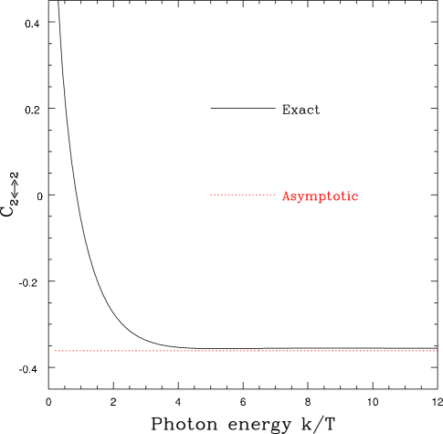
FIG. 5.: Contribution $C_{2\leftrightarrow 2}(k/T)$ to the constant under the log arising from $2\leftrightarrow 2$ particle processes (gluon-photon Compton scattering and quark-antiquark annihilation), as a function of $k/T$. The dotted line is the asymptotic limit, derived by [9, 10]. The result is quite close to the asymptotic value already at $k/T=3$; the visible but tiny difference between the curve and the asymptotic value is due to a $1/k$ tail with a very small coefficient.

The functions $C_{\rm brem}(k/T)$ and $C_{\rm annih}(k/T)$ are $\kappa$ dependent. We show $C_{\rm brem}(k/T)$ [defined as the contribution to the integral (LABEL:eq:outer_int) from the regions ${p_{\parallel}}>0$ plus ${p_{\parallel}}<-k$], and $C_{\rm annih}(k/T)$ [the $-k<{p_{\parallel}}<0$ contribution to Eq. (LABEL:eq:outer_int)] separately in Fig. 6, for a number of physically interesting values of $\kappa$. The values shown were selected to equal the value for an Abelian electron plasma ($\kappa=3/4$), an electron plus muon plasma ($\kappa=3/8$), and a quark-gluon plasma with 2 to 6 flavors ($\kappa=2/(6+N_{\rm f})$). For the Abelian plasmas, the photon dispersion correction is included in $\delta E$ [c.f. Eq. (38)], which suppresses soft bremsstrahlung.

The effect of LPM suppression on the bremsstrahlung and inelastic pair annihilation rates is shown in Fig. 7, which plots the ratio of the actual bremsstrahlung and inelastic pair annihilation rates to the corresponding rates neglecting the LPM effect, for the case of $N_{\rm f}=2$ QCD. For most momenta, it is evident that the LPM suppression is a rather modest 35% or less. The exception, for the range of photon momenta shown ($k<10\,T$), is bremsstrahlung with $k\mbox{~{}{\raisebox{1.72218pt}{$<$}} {\raisebox{-2.58334pt}{$\sim$}}~{}}2\,T$. Here the LPM effect is important. It also makes a large relative suppression to the rate for inelastic pair annihilation at very large $k/T$, but in practice this means $k>20\,T$, where the statistical factor $n_{f}(k)\sim e^{-k/T}$ ensures that virtually no photons are produced.

   

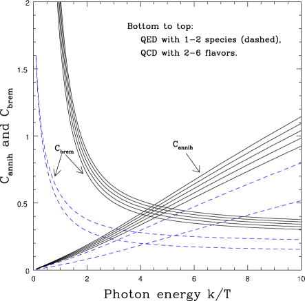
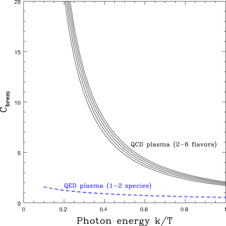
FIG. 6.: Left panel: Contributions $C_{\rm brem}(k/T)$ and $C_{\rm annih}(k/T)$ to the constant under the log arising from near-collinear bremsstrahlung and pair production. The curves rising at small $k/T$ are plots of $C_{\rm brem}(k/T)$, while the curves rising at large $k/T$ are plots of $C_{\rm annih}(k/T)$. In both cases, the curves from bottom to top are for $\kappa={}$3/4, 3/8, 1/4, 2/9, 1/5, 2/11, and 1/6, corresponding to electron plasma, electron plus muon plasma, and QCD with 2, 3, 4, 5, or 6 quark flavors, respectively. In the bottom two curves, we include the plasma induced photon dispersion, relevant for QED plasmas, which suppresses the soft bremsstrahlung rate. Right panel: Magnified view of the soft photon region of the bremsstrahlung contribution.

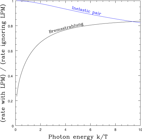
FIG. 7.: Relative importance of the LPM effect. The figure shows the ratio of the true bremsstrahlung and inelastic pair annihilation rates to the rates which result if one neglects the LPM effect in the treatment, for the case of $\kappa=1/4$ which corresponds to two flavor QCD. The LPM suppression is rather modest, 30% or less, except for bremsstrahlung photons of energy $k\mbox{~{}{\raisebox{1.72218pt}{$<$}} {\raisebox{-2.58334pt}{$\sim$}}~{}}2\,T$. These plots show very little change for other values of the mass ratio $\kappa$.

   

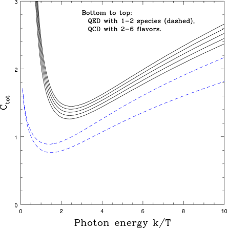
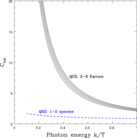
FIG. 8.: Left panel: Total constant under the log, equal to the sum of contributions $C_{\rm tot}(k/T)\equiv$ ${\textstyle{1\over 2}}\log(2k/T)+C_{2\leftrightarrow 2}(k/T)+C_{\rm brem}(k/T)+C_{\rm annih}(k/T)$. This is the value which must be added to $\ln(T/m_{\infty})$ to obtain the total emission rate, as indicated in Eq. (85). The different curves (from bottom to top) are the same as in Fig. 6. Right panel: Magnified view of the soft photon region.

The complete constant under the log, $C_{\rm tot}(k/T)$, equal to the sum of contributions shown in Eq. (86), is plotted in Fig. 8. Over a wide range of photon energies, $T\mbox{~{}{\raisebox{1.72218pt}{$<$}} {\raisebox{-2.58334pt}{$\sim$}}~{}}k\mbox{~{}{\raisebox{1.72218pt}{$<$}} {\raisebox{-2.58334pt}{$\sim$}}~{}}6T$, one sees that $C_{\rm tot}(k/T)$ lies between about 1 and 2.

Finally, Fig. 9 shows the full leading-order photon emission rate, together with the bremsstrahlung, inelastic pair annihilation  and $2\leftrightarrow 2$ contributions, for two-flavor QCD with $\alpha_{\rm s}=0.2$. The left panel shows the production rate $d\Gamma_{\gamma}/dk$, while the right panel shows the rate weighted by a factor of the photon energy. One sees that bremsstrahlung is the dominant production mechanism for not-so-hard photons with $k<2T$. As discussed in section III, the ratio of the bremsstrahlung rate to the $2\leftrightarrow 2$ rate scales, at small $k$, as $(T/k)^{3/2}$ (up to logs), a factor of $\sqrt{k/T}$ less strongly than if there were no LPM effect. At intermediate values of $k/T\mbox{~{}{\raisebox{1.72218pt}{$>$}} {\raisebox{-2.58334pt}{$\sim$}}~{}}4$, where the most experimentally detectable photons are probably produced, the $2\leftrightarrow 2$ processes generate the largest contribution, comparable to the sum of the two near-collinear inelastic processes. At large $k\gg T$, the inelastic pair annihilation emission rate grows, in comparison to the $2\leftrightarrow 2$ rate, almost linearly with $k/T$ up to quite large $k$. As shown in section III, the ratio of these rates ultimately grows only as $(k/T)^{1/2}$ but this asymptotic behavior turns out to set in only for $k>10\,T$.

   

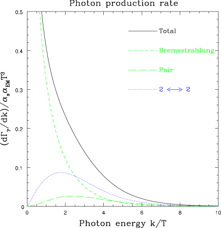
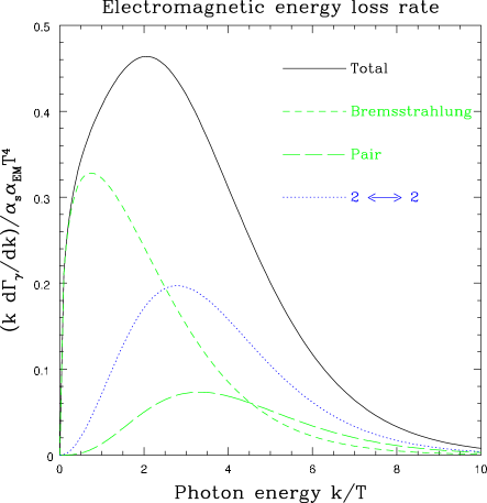
FIG. 9.: Total photon emission rate, together with the bremsstrahlung, inelastic pair annihilation  and $2\leftrightarrow 2$ contributions, for two-flavor QCD with $\alpha_{\rm s}=0.2$. The left panel shows $d\Gamma_{\gamma}/dk$, divided by $\alpha_{\rm s}\,\alpha_{\rm EM}\,T^{3}$, while the right panel shows rates weighted by photon energy.

VII Conclusions

The above results represent the first complete leading order calculation of the photon emission rate from a hot, weakly coupled, thermalized quark gluon plasma at zero chemical potential. In addition to well known $2\leftrightarrow 2$ particle processes, near-collinear bremsstrahlung and inelastic pair annihilation also make leading order contributions. A consistent treatment of these latter processes requires a rather complicated analysis in order to incorporate correctly the effects of multiple soft scatterings which may occur during the emission of the photon. These lead to an $O(1)$ suppression of these near-collinear processes. To account for this suppression, known as the LPM effect, we solved the integral equation, derived in Ref. [19], which accounts for partial coherence between successive scattering events.

For modest values of $\alpha_{\rm s}\sim 0.2$, we find that near-collinear bremsstrahlung dominates the photo-emission rate for soft photons with energy $k\mbox{~{}{\raisebox{1.72218pt}{$<$}} {\raisebox{-2.58334pt}{$\sim$}}~{}}2T$, and inelastic pair annihilation dominates the rate for very hard photons, $k\gg 10\,T$. For intermediate values of $k$, which is the most easily detected range of photon energies, the $2\leftrightarrow 2$ processes are of comparable importance to the sum of the near-collinear inelastic processes. The LPM suppression is substantial precisely where the inelastic mechanisms are dominant, but is fairly mild for intermediate values of photon energy. Parametrically, the soft photon emission rate behaves as $d\Gamma_{\gamma}\propto k^{-1/2}\,dk$, which is less infrared singular, by a square root of $k$, from the result found in Refs. [26] and [12] which neglect the LPM effect.

REFERENCES

[1]
E. V. Shuryak,
Phys. Lett. B 78, 150 (1978)
[Sov. J. Nucl. Phys. 28, 408.1978 YAFIA,28,796 (1978)].
[2]
K. Kajantie and H. I. Miettinen,
Z. Phys. C 9, 341 (1981).
[3]
K. Kajantie and P. V. Ruuskanen,
Phys. Lett. B 121, 352 (1983).
[4]
F. Halzen and H. C. Liu,
Phys. Rev. D 25, 1842 (1982).
[5]
B. Sinha,
Phys. Lett. B 128, 91 (1983).
[6]
R. C. Hwa and K. Kajantie,
Phys. Rev. D 32, 1109 (1985).
[7]
G. Staadt, W. Greiner and J. Rafelski,
Phys. Rev. D 33, 66 (1986).
[8]
M. Neubert,
Z. Phys. C 42, 231 (1989).
[9]
J. Kapusta, P. Lichard and D. Seibert,
Phys. Rev. D 44, 2774 (1991)
[Erratum–ibid. D 47, 4171 (1991)].
[10]
R. Baier, H. Nakkagawa, A. Niegawa and K. Redlich,
Z. Phys. C 53, 433 (1992).
[11]
H. A. Weldon,
Phys. Rev. D 26, 2789 (1982).
[12]
P. Aurenche, F. Gelis, R. Kobes and H. Zaraket,
Phys. Rev. D 58, 085003 (1998)
[hep-ph/9804224].
[13]
P. Aurenche, F. Gelis and H. Zaraket,
Phys. Rev. D 61, 116001 (2000)
[hep-ph/9911367].
[14]
P. Aurenche, F. Gelis and H. Zaraket,
Phys. Rev. D 62, 096012 (2000)
[hep-ph/0003326].
[15]
F. D. Steffen and M. H. Thoma,
Phys. Lett. B 510, 98 (2001)
[hep-ph/0103044].
[16]
L. D. Landau and I. Pomeranchuk,
Dokl. Akad. Nauk Ser. Fiz. 92 (1953) 535;
L. D. Landau and I. Pomeranchuk,
Dokl. Akad. Nauk Ser. Fiz. 92 (1953) 735.
[17]
A. B. Migdal, Doklady Akad. Nauk S. S. S. R. 105, 77 (1955).
[18]
A. B. Migdal,
Phys. Rev. 103, 1811 (1956).
[19]
P. Arnold, G. D. Moore, and L. G. Yaffe,
“Photon Emission from Ultrarelativistic Plasmas,”
[hep-ph/0109064].
[20]
B. G. Zakharov,
JETP Lett. 63, 952 (1996)
[hep-ph/9607440];
ibid.65, 615 (1997)
[hep-ph/9704255];
Phys. Atom. Nucl. 61 (1998) 838
[Yad. Fiz. 61 (1998) 924]
[hep-ph/9807540].
[21]
R. Baier, Y. L. Dokshitzer, A. H. Mueller and D. Schiff,
Nucl. Phys. B 531 (1998) 403
[hep-ph/9804212].
[22]
R. Baier, D. Schiff and B. G. Zakharov,
Ann. Rev. Nucl. Part. Sci. 50, 37 (2000)
[hep-ph/0002198].
[23]
B. G. Zakharov,
hep-ph/9807396;
JETP Lett. 73, 49 (2001)
[Pisma Zh. Eksp. Teor. Fiz. 73, 55 (2001)]
[hep-ph/0012360].
[24]
R. Baier, Y. L. Dokshitzer, S. Peigne and D. Schiff,
Phys. Lett. B 345, 277 (1995)
[hep-ph/9411409];
Phys. Rev. C 60, 064902 (1999)
[hep-ph/9907267].
[25]
R. Baier, Y. L. Dokshitzer, A. H. Mueller, S. Peigne and D. Schiff,
Nucl. Phys. B 483, 291 (1997)
[hep-ph/9607355];
ibid.484, 265 (1997)
[hep-ph/9608322].
[26]
P. Aurenche, F. Gelis, R. Kobes and E. Petitgirard,
Phys. Rev. D 54, 5274 (1996)
[hep-ph/9604398].
[27]
R. Blankenbecler and S. D. Drell,
Phys. Rev. D 53, 6265 (1996).
[28]
R. Baier, Y. L. Dokshitzer, A. H. Mueller, S. Peigne and D. Schiff,
Nucl. Phys. B 478, 577 (1996)
[hep-ph/9604327].
[29]
B. G. Zakharov,
Pisma Zh. Eksp. Teor. Fiz. 64, 737 (1996)
[JETP Lett. 64, 781 (1996)]
[hep-ph/9612431];
B. G. Zakharov,
Phys. Atom. Nucl. 62, 1008 (1999)
[Yad. Fiz. 62, 1075 (1999)]
[hep-ph/9805271];
ibid.61, 838 (1998)
[hep-ph/9807540].
[30]
H. A. Weldon,
Phys. Rev. D 26, 1394 (1982).
[31]
P. Arnold, G. D. Moore and L. G. Yaffe,
JHEP 0011, 001 (2000)
[hep-ph/0010177].
[32]
G. D. Moore,
JHEP 0105, 039 (2001)
[hep-ph/0104121].