MPI-PhT 2001-45

Gauged Inflation

Ralf Hofmann and Mathias Th. Keil

Max-Planck-Institut für Physik
Werner-Heisenberg-Institut
Föhringer Ring 6, 80805 München
Germany

We propose a model for cosmic inflation which is based on an effective description of strongly interacting, nonsupersymmetric matter within the framework of dynamical Abelian projection and centerization. The underlying gauge symmetry is assumed to be $SU(N+1)$ with $N\gg 1$. Appealing to a thermodynamical treatment, the ground-state structure of the model is classically determined by a potential for the inflaton field (dynamical monopole condensate) which allows for nontrivially BPS saturated and thereby stable solutions. For $T<M_{P}$ this leads to decoupling of gravity from the inflaton dynamics. The ground state dynamics implies a heat capacity for the vacuum leading to inflation for temperatures comparable to the mass scale $M$ of the potential. The dynamics has an attractor property. In contrast to the usual slow-roll paradigm we have $m\gg H$ during inflation. As a consequence, density perturbations generated from the inflaton are irrelevant for the formation of large-scale structure, and the model has to be supplemented with an inflaton independent mechanism for the generation of spatial curvature perturbations. Within a small fraction of the Hubble time inflation is terminated by a transition of the theory to its center symmetric phase. The spontaneously broken $Z_{N+1}$ symmetry stabilizes relic vector bosons in the epochs following inflation. These heavy relics contribute to the cold dark matter of the universe and potentially originate the UHECRs beyond the GZK bound.

1 Introduction

Inflationary cosmology was invented to resolve a number of problems posed by the conventional hot big bang scenario [1, 2]. Experimental facts not explained by the old cosmology were (A) the apparent spatial flatness of the universe, (B) the nondetection of magnetic monopoles stemming from the spontaneous symmetry breaking in grand unified gauge theories (GUTs) at a scale of $\sim 10^{16}$ GeV, and (C) the horizon problem, arising from the extreme isotropy of the cosmic microwave background radiation (CMBR). In addition, it was hoped that the mechanism responsible for inflation could also provide the small density perturbations needed to seed large-scale structure formation (D).

Superluminal expansion of the universe by a factor of about $\mbox{e}^{60}$ at a sub-Planckian epoch can solve the flatness problem (A) [3]. To meet the constraints on postinflationary density perturbations, however, the new inflationary cosmology of [2] needs densities at inflation much smaller than $10^{-10}\times M^{4}_{P}$ [5]. This, in turn, would cause the collapse of a typical closed universe before it could inflate. A resolution of this problem was proposed by assuming chaotic inflation [3]. We will argue in this paper that even within the new inflationary scenario collapse can be avoided if the initial radius $a_{0}$ of a closed universe lies above some critical value.

The monopole problem (B) is resolved if inflation sets in at scales considerably smaller than the GUT scale. In models where inflation is driven by a single, minimally coupled, classical, real scalar field (inflaton), either the potential for this field is constructed to allow for a regime of slow-roll, which implies a small mass $m$ for the field fluctuations if compared to the Hubble parameter $H$ [2], or a nonconventional kinetic term for this field is introduced in the action [6]. However, the recent work of [4] discusses also fast-roll inflation. The realization within the context of the present work is that slow-roll does not necessarily imply the hierarchy of mass scales in the inflaton sector which is expressed by $m\ll H$.

Inflation also solves the horizon problem (C) since it implies that todays observable universe was entirely contained in a causally connected patch of space prior to inflation.

Assuming $m\ll H$ during inflation, the problem of density perturbations (D) was addressed in the past by considering quantum fluctuations of the inflaton field which adiabatically freeze into a scale invariant spectrum of classical fluctuations upon horizon-exit during inflation. Theses fluctuations, when re-entering the horizon after inflation, were thought to be responsible for the density perturbations seeding the formation of large-scale structure. It was only recently that alternatives to $m\ll H$ have been put forward in the literature [7]. Post-inflationary density perturbations are explained by the decay of a moduli field whose existence and dynamics is independent from the inflaton sector. Our proposed model relies on the existence of this extra field but, at the same time, assures that moduli fields are not generated as a consequence of the inflaton dynamics. This resolves the conventional moduli problem [8, 9].

We propose a large-$N$, pure $SU(N+1)$ gauge theory to be responsible for the dynamics leading to inflation and terminating it. The idea is that at the time when the universe enters the post-Planckian epoch the physics of matter is dominated by a large gauge symmetry which, in the course of cosmic evolution, dynamically freezes more and more of its subgroups to their respective centers hence generating an ever increasing number of mass scales. The first center transition is the mechanism proposed here to terminate the first regime of quasi-exponential expansion. We identify this regime with usual inflationary cosmology. The question how fermions appear and enter the dynamics will not be addressed in this work.

In order to be able to access the complicated vacuum structure of $SU(N+1)$ gauge theory we resort to a conjectured, effective description based on the picture of a dual superconductor (Abelian Higgs model) at high temperature $T$ [10] and based on confinement of fundamental test charges due to the condensation of center vortices at low energy [11] ($Z_{N+1}$ symmetric Higgs sector). On the one hand, this picture is supported by lattice simulations of $SU(2)$ pure gauge theory [12]. On the other hand, models based on center-vortex condensation are quite successful in explaining the low-energy features of the QCD vacuum [13]. In the following we will refer to the complex Higgs field as “inflaton field.”

In the high $T$ regime the surviving gauge group should be maximally Abelian, i.e. $U(1)^{N}$. This renders the vacuum a condensate of magnetic monopoles being charged under $N$ different $U(1)$ groups. For simplicity we restrict ourselves to a higgsed model of a single $U(1)$ group which still is in accord with the qualitative picture [14]. At low energy a spontaneously broken $Z_{N+1}$ symmetry will be apparent for the same field $\phi$ that described monopole condensation at high $T$. Thereby, the distinction of high and low energy is given by the single mass scale $M$ of the potential. This potential is constructed to allow for BPS saturated [15] Euclidean ground state dynamics at high $T$. In the course of cosmological evolution it smoothly enters a regime $T\simeq M$ where a description in Minkowskian signature becomes necessary due to destruction of thermal equilibrium by transition to the center symmetry. BPS saturation at high $T$ suppresses the gravitational coupling term in the second-order (Euclidean) equations for the Higgs field, topologically stabilizes the dynamics, justifies the classical (effective) description, and leads to the appearance of a temperature dependent cosmological constant [14].

Much in contrast to perturbatively obtained effective potentials we have no explicit $T$ dependence in our potential. Rather, the $T$ dependence of physical quantities, such as the energy density of the vacuum, arises entirely from the $T$ dependence of the solutions to the field equations.

Assuming Einstein gravity to hold, the cosmic evolution of an isotropic and homogeneous universe is governed by the Friedmann equations. In our approach the source terms are the black body radiation of the massive gauge field quanta (scalar quanta are of mass considerably larger than temperature and hence much heavier than the vector bosons) and the aforementioned cosmological constant $\Lambda=\Lambda(T)$.

The pattern of symmetry breaking induced by the cooling universe is: Unbroken gauge symmetry at temperatures $T\gg M$ $\rightarrow$ increasing spontaneous gauge symmetry breaking by a growing inflaton amplitude in an intermediate regime $\rightarrow$ explicit breaking of the $U(1)$ gauge symmetry to its discrete subgroup $Z_{N+1}$ for field amplitudes close to $M$. This is a concrete realization of Krauss’ and Wilzcek’s observation that fundamental gauge symmetries masquerade as discrete symmetries for observers at low energies [16].

The evolution of the scale factor $a$ can be summarized as: radiation dominated, slow power-law expansion $\rightarrow$ energy density of the vacuum becomes comparable with that of radiation implying stronger power-law expansion $\rightarrow$ quasi-exponential expansion due to vacuum dominance (inflation) $\rightarrow$ thermal nonequilibrium due to the termination of inflation by vacuum decay and creation of new particles (pre- and reheating). Inflationary relics are vector particles of mass $\sim M$ whose relative stability is protected by a discrete symmetry $Z_{N+1}$ [16, 17].

The paper is organized as follows: In Section 2 we introduce the model. Thermal equilibrium prior to and during a large part of inflation implies a description in Euclidean space with a compactified time dimension of length $\beta\equiv T^{-1}$. At several occasions we exploit the fact that observables such as the energy-density of the vacuum or the Hubble parameter being time-independent in Euclidean signature have a trivial analytical continuation to Minkowskian signature. Requiring the inflaton field to be BPS saturated in a non-trivial way for the regime governed by the $U(1)$ gauge symmetry, severely constrains the corresponding potential. Demanding in addition that there is a smooth transition to the center symmetric regime, which is determined by a single mass scale $M$, fixes the inflaton potential uniquely. After the construction of the potential we solve the dynamics of the ground state which is assumed to be locally Lorentz invariant. As a result, we obtain a cosmological constant $\Lambda$ depending linearly on $T$. Four-momentum conservation in a Friedmann universe, whose evolution is determined by (massive) black body radiation of the gauge field excitations and $\Lambda=\Lambda(T)$, determines $\Lambda$ as a function of $a$. We find that the inflaton amplitude at inflation is a fixed point of cosmic evolution.

In Section 3 we obtain the time evolution of $a$. We show that all phenomenological requirements for inflationary cosmology can be met provided an additional light scalar field is invoked to generate the density perturbations demanded by the CMBR anisotropy and the constraints imposed by models of large-scale structure formation. General implementations of this additional scalar have recently been discussed [7]. Moreover, we prove that a closed and initially large enough universe of sub-Planckian density does not collapse but may also inflate.

An investigation of the physics terminating inflation is performed in Section 4. At the point $|\phi|_{c}$, where the breaking of continuous gauge symmetry becomes noticeable, i.e. where $\left.\partial_{|\phi|}^{2}V(|\phi|)\right|_{|\phi|=|\phi|_{c}}=0$ for the first time, thermal equilibrium is destroyed due to the inflaton amplitude becoming time dependent even in the Euclidean and due to tachyonic excitations. This leads to a termination of inflation by tachyonic preheating and the subsequent generation of new matter. Due to a spontaneously broken $Z_{N+1}$ symmetry there are no Goldstone modes. Therefore, no isothermal density fluctuations can be produced from the dynamics driving and terminating inflation. In Section 5 we summarize the results, speculate on implications of this work, and provide an outlook.

2 The model

2.1 BPS saturated thermodynamics: The ground state

The central assumption of our model is that very early cosmology effectively is driven by a gauged $U(1)$ theory of a classical and complex “inflaton field.” The scalar as well as the gauge sector of the model are taken to be minimally coupled to Einstein gravity. The corresponding action is

$$S=\int d^{4}x\sqrt{-g}\left[-\frac{1}{16\pi G}R-\frac{1}{4}F_{\mu\nu}F^{\mu\nu}+\overline{{\cal D}_{\mu}\phi}{\cal D}^{\mu}\phi-V(\bar{\phi}\phi)\right]\,,$$ (1)

where ${\cal D}_{\mu}\equiv\partial_{\mu}+ieA_{\mu}$ denotes the gauge covariant derivative, and $V$ is an effective potential to be specified later. Assuming thermal equilibrium, the dynamics is considered for a compact time dimension in Euclidean signature $0\leq\tau\leq\beta\equiv 1/T$.

According to the standard cosmological assumptions of spatial homogeneity and isotropy the inflaton field $\phi$ is independent of the spatial variables but may depend on the Euclidean time coordinate. It will be shown below that the vacuum is dominated by the BPS saturated dynamics of $\phi$ alone, which is solved in a gauge allowing for physical boundary conditions. Therefore one may regard the gauge field dynamics in the background of the inflaton solution.

What about gravitational deformation? Gravity is represented by the Euclidean version of the Robertson-Walker metric with scale factor $a$, while $\phi$ and $\bar{\phi}$ satisfy the BPS equations

$$\partial_{\tau}\phi=\bar{V}^{1/2}\,,\ \ \ \ \partial_{\tau}\bar{\phi}={V}^{1/2}\ ,$$ (2)

where $V\equiv\bar{V}^{1/2}{V}^{1/2}$. Taking the divergences of the vector equations $v_{\mu}=\delta_{\mu\tau}\partial_{\tau}\phi=\delta_{\mu\tau}\bar{V}^{1/2}$ and $\bar{v}_{\mu}=\delta_{\mu\tau}\partial_{\tau}\bar{\phi}=\delta_{\mu\tau}{V}^{1/2}$ yields

$$\nabla_{\mu}v_{\mu}=\nabla_{\tau}\bar{V}^{1/2}+3H\bar{V}^{1/2}\ ,\ \ \ \ \nabla_{\mu}\bar{v}_{\mu}=\nabla_{\tau}{V}^{1/2}+3H{V}^{1/2}\ ,$$ (3)

where $\nabla_{\mu}v^{\nu}=\partial_{\mu}+\Gamma^{\nu}_{\mu\kappa}v^{\kappa}$ denotes the action of the gravitational covariant derivative and $H\equiv\frac{da/d\tau}{a}$ is the Euclidean Hubble parameter. Since the covariant time derivatives on the right-hand sides (RHSs) of eqs. (3) act on scalars we can replace them by ordinary time derivatives. Using the BPS equations (2) and the definitions of ${V}^{1/2}$ and $\bar{V}^{1/2}$, we can express the RHSs of eq. (3) as

$$\frac{\partial\bar{V}^{1/2}}{\partial\bar{\phi}}{V}^{1/2}+3H\bar{V}^{1/2} = V^{-1/2}\frac{\partial V}{\partial\bar{\phi}}V^{1/2}+3H\bar{V}^{1/2}=\frac{\partial V}{\partial\bar{\phi}}+3H\bar{V}^{1/2}\,,$$

$$\frac{\partial{V}^{1/2}}{\partial{\phi}}\bar{V}^{1/2}+3H{V}^{1/2} = \bar{V}^{-1/2}\frac{\partial V}{\partial\phi}\bar{V}^{1/2}+3H{V}^{1/2}=\frac{\partial V}{\partial\phi}+3H{V}^{1/2}\ .$$ (4)

Invoking eq. (3), we realize that $\bar{\phi}$ and $\phi$ would approximately satisfy the Euclidean, second order field equations if the gravitational coupling terms in eqs. (2.1) are small compared to $\partial_{\phi}V$ for the relevant range of $|\phi|\leq|\phi|_{c}$. We show this in Sec 3.2. Apparently, $\bar{V}^{1/2}$ and ${V}^{1/2}$ are only fixed up to constant phases $\mbox{e}^{i\delta}$ and $\mbox{e}^{-i\delta}$, respectively. This freedom does not survive if the solution of the ground state dynamics is based on inflaton dominance (see below).

Let us now construct the potential $V$. We demand $(i)$ the existence of non-trivial BPS saturated solutions along the compact, Euclidean time coordinate in the regime of $U(1)$ gauge symmetry and a smooth transition to the $Z_{N+1}$ symmetric regime. $(ii)$ In addition we require the potential to be characterized by a single mass scale $M$. Detailed justifications can be found in [14].

$(i)$ fixes the potential as (see also [18])

$$V(\bar{\phi}\phi)=\frac{M^{6}}{\bar{\phi}\phi}+\lambda^{2}M^{-2(N-2)}(\bar{\phi}\phi)^{N}-2\,\lambda M^{5-N}\frac{1}{\bar{\phi}\phi}\mbox{Re}\,\phi^{N+1}\ ,$$ (5)

where $\lambda$ denotes a dimensionless coupling constant. In the limit $N\to\infty$ the potential is gauge invariant for the whole $\phi$ range. However, the transition to the trivial vacuum is not smooth, violating $(i)$. For finite $N$ the $N+1$ points of zero energy are given by the $N+1$ unit roots times $M/\lambda^{1/(N+1)}$. In order to meet $(ii)$ we have to set $\lambda=1$. We stress that adding a constant to the potential would destroy $(i)$. Therefore, the corresponding contribution to the cosmological constant vanishes after the transition to the center symmetric regime! In section 2.3 we will see that demanding the inflationary fixed point $|\phi|_{i}$ to coincide with the potential’s first point of inflexion $|\phi|_{c}$ (onset of tachyonic excitations) yields $N\sim 34$. The relative deviation of the pole part and the full potential at this point is about 1%. Therefore, even at finite and not too small $N$ and for $|\phi|<|\phi|_{c}$ we may regard the potential eq. (5) as gauge invariant and given by the pure pole term whereas $Z_{N+1}$ symmetry is apparent for $|\phi|>|\phi|_{c}$. A graph of the potential is shown in Fig. 1.

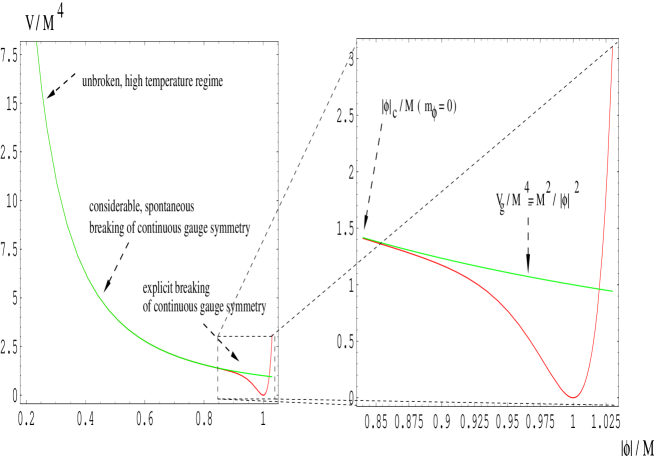
Figure 1: The potential $V(|\phi|^{2})$ of eq. (5) allowing for BPS saturated solutions along the Euclidean, compact time dimension. We have set $N=34$ and $\lambda=1$. In the enlarged region, where the continuous gauge symmetry is broken explicitly, the gauge invariant, pure pole part $V_{g}$ deviates strongly from the full potential.

We now turn to the solution of the ground state dynamics at high $T$. As mentioned above, our ansatz is a dominant inflaton field. The idea is to choose the gauge such as to shuffle a maximum of physics into the scalar sector. In this sense a chosen gauge at finite temperature is physical if and only if the solution $\phi$ to eq. (2) is periodic.

We now show that the choice of phase in the BPS equations is correlated with a choice of gauge. For example, imposing unitary gauge $\phi=|\phi|$ before solving the BPS equations (2), $\bar{V}^{1/2}$ and ${V}^{1/2}$ must be real, leading to the following solution

$$\phi(\tau)=\sqrt{\phi^{2}_{0}+2M^{3}(\tau-\tau_{0})}\ .$$ (6)

Obviously this is not a periodic function. The only choices of phase yielding the following periodic solutions [19]

$$\phi^{(n)}(\tau)=\sqrt{\frac{M^{3}\beta}{2|n|\pi}}\,\mbox{e}^{2n\pi i\frac{\tau}{\beta}}\ ,\ \ (n\in{\bf Z})\$$ (7)

correspond to

$$V^{1/2}(\phi)=\pm i\frac{M^{3}}{\phi}\,,\ \ \ \ \bar{V}^{1/2}(\phi)=\mp i\frac{M^{3}}{\bar{\phi}}\,,\ \$$ (8)

for $(|\phi|<|\phi|_{c})$. In eq. (7) the integer $n$ counts the number of times the corresponding solution winds around the pole of the potential. Note that for a given topological sector the BPS saturated solution is the one with lowest spatial action density and thus it is stable [19]. In what follows we will restrict ourselves to $n=1$.

After solving eq. (2) we now show that the Maxwell equations with the source current

$$j_{\mu}\equiv ie\,\delta_{\mu 0}\ \left[{\bar{\phi}}^{(1)}\stackrel{{\scriptstyle\rightarrow}}{{\cal D}}_{\tau}\phi^{(1)}-\left(\overline{\phi^{(1)}\stackrel{{\scriptstyle\leftarrow}}{{\cal D}}_{\tau}}\right)\phi^{(1)}\right]$$ (9)

can be solved by the pure gauge $A_{\mu}=\delta_{\mu 0}A(\tau)$, in accord with local Lorentz invariance of the ground state. Maxwell’s equations in a gravitational background read [21]

$$\partial_{\mu}\left[\,\sqrt{\tilde{g}}F_{\mu\nu}\,\right]=j_{\nu}\ ,$$ (10)

where $\tilde{g}$ is the determinant of the metric tensor with Euclidean signature. From eqs. (9,10) it is clear that $A_{\mu}$ being pure gauge implies the vanishing of ${\cal D}_{\tau}\phi^{(1)}$. Hence all we have to do is to show in a conveniently chosen gauge that with the background configuration of eq. (7) for $n=1$ there exists a pure gauge of the form $A_{\mu}=\delta_{\mu 0}A(\tau)$ with ${\cal D}_{\tau}\phi^{(1)}=0$. This is most obvious in unitary gauge $\phi^{(1)}=|\phi^{(1)}|$ where according to eq. (7) we have $\partial_{\tau}\phi^{(1)}=0$. Hence, ${\cal D}_{\tau}\phi^{(1)}=0$ for $A(\tau)\equiv 0$.

We now show that the back reaction of the vacuum gauge field onto the vacuum scalar dynamics is zero, at least in the sense of an average. Since the $\tau$ dependence of the solution eq. (7) resides only in its phase, observables do not depend on $\tau$. So averaging over the cycle leaves the potential invariant. Although the gauge covariant BPS equations

$${\cal D}_{\tau}\phi=\bar{V}^{1/2}\,,\ \ \ \ \overline{{\cal D}_{\tau}\phi}={V}^{1/2}$$ (11)

are not satisfied by the above field configurations, their cycle average is. Using eqs. (2) the cycle average can easily be shown to vanish

$$ie\int_{0}^{\beta}d\tau\,A_{\tau}\phi^{(1)}(\tau)=i\frac{2\pi}{\beta}\sqrt{\frac{M^{3}\beta}{2\pi}}\,\int_{0}^{\beta}d\tau\,\mbox{e}^{2\pi i\tau/\beta}=0\;.\$$ (12)

Since we have

$$\frac{m_{A}}{m_{\phi}}=\frac{e}{\sqrt{6}}\,\left(\frac{|\phi|}{M}\right)^{3}$$ (13)

scalar modes are much heavier than the vector bosons within the entire relevant range of $\phi$ amplitudes. Hence, the inflaton is a slow variable as compared to the vector field. Therefore, the employed procedure to solve the vacuum dynamics of the model is a Born-Oppenheimer approximation. Also, possible scalar excitations have mass much larger than $T$ for $|\phi|<|\phi_{c}|$ which allows for a classical treatment of the ground state dynamics [14].

We are now in a position to perform a trivial analytical continuation of the Euclidean action to Minkowskian signature by letting $\tau\rightarrow-it$. The kinetic term $\overline{{\cal D}_{\tau}\phi}{\cal D}_{\tau}\phi$ remains zero. Therefore, we derive a $T$ dependent cosmological constant

$$\Lambda=\Lambda(T)\equiv V(|\phi^{(1)}|^{2})=2\pi M^{3}T\ .$$ (14)

This result may be puzzling for the reader. We have derived a finite heat capacity of the vacuum without ever referring to a density matrix. Let us explain this fact. It is useful to think of the vacuum at temperature $T$ as a medium with a constant heat capacity which is carried by microscopic degrees of freedom being of a very different nature than the (irrelevant) quanta of the inflaton field ($m_{\phi}/T\sim 15.4$!). If we could probe with a resolution much greater than $T$ we would observe the microscopic dynamics directly and most probably find effects that even break local Lorentz invariance. However, this high resolution is not available and so the ground state at resolution $T$ deserves to be called a vacuum. The memory of high-scale quantum dynamics is contained in the shape of the effective potential [14]. A way to picture this is an analogy with the condensed state represented by a piece of metal. In this case the macroscopic property heat capacity is explained by quasidegrees of freedom — phonons and valence electrons. In an effective, macroscopic description these underlying degrees of freedom are integrated out.

2.2 Gravitational sources

We now investigate the implications of the above vacuum dynamics for the energy balance in a Friedmann universe at high $T$. Cosmology will not only be affected by the vacuum structure but also by thermal excitations. The Higgs mechanism induces a mass $m_{A}=e|\phi|$ for the gauge field. If $m_{A}\ll T$ the spectrum of these excitations can be approximated by black body radiation, and we can take the mass $m_{A}$ into account perturbatively when calculating the energy density $\varepsilon_{A}$ and the pressure $p_{A}$. In principle, there is the possibility of inflaton excitations. Their mass $m_{\phi}=\partial^{2}_{|\phi|}V(|\phi|^{2})$ is much larger than $T$ for $|\phi|$ away from $|\phi|_{c}$ [14]. Hence, we may disregard scalar excitations (Section 4). Considering three polarization states of the massive vector bosons, expanding up to order $m_{A}^{2}$, and expressing mass in terms of temperature by virtue of eq. (7), we obtain

$$\varepsilon_{A}=\frac{\pi^{2}}{10}T^{4}-\frac{e^{2}}{16\pi}M^{3}T\ ,\ \ \ \ p_{A}=\frac{\pi^{2}}{30}T^{4}-\frac{e^{2}}{24\pi}M^{3}T\ .$$ (15)

The matter of the universe is a perfect fluid with energy density $\varepsilon$ and pressure $p$ given as

$$\varepsilon=\varepsilon_{A}+\Lambda\ ,\ \ \ \ \ p=p_{A}-\Lambda\ ,$$ (16)

where the equation of state $\Lambda=\varepsilon_{\Lambda}=-p_{\Lambda}$ of a cosmological constant has been used. Using $\Lambda\equiv V(|\phi^{(1)}|^{2})$ and eq. (15), we can write $\varepsilon$ and $p$ as functions of $\Lambda$, namely,

$$\varepsilon=\frac{\Lambda^{4}}{160\pi^{2}M^{12}}+\kappa_{1}\Lambda\ ,\ \ \ \ p=\frac{\Lambda^{4}}{480\pi^{2}M^{12}}-\kappa_{2}\Lambda\ ,$$ (17)

where

$$\kappa_{1}\equiv 1-\frac{e^{2}}{32\pi^{2}}\ ,\ \ \ \kappa_{2}\equiv 1+\frac{e^{2}}{48\pi^{2}}\ .$$ (18)

We are now in a position to solve the Friedmann equations. Here, we are in particular concerned with the equation governing energy-momentum conservation [21]

$$\frac{d}{da}\left(\varepsilon\,a^{3}\right)=-3\,a^{2}\,p\ .$$ (19)

Upon use of eq. (17) together with eq. (19) we obtain

$$\frac{d}{da}\Lambda=-\frac{\Lambda}{a}\,\frac{\frac{\Lambda^{3}}{40\pi^{2}M^{12}}+3(\kappa_{1}-\kappa_{2})}{\frac{\Lambda^{3}}{40\pi^{2}M^{12}}+\kappa_{1}}\ .$$ (20)

2.3 Attractor property of inflaton dynamics

Equation 20 is solved by

$$\frac{a}{a_{0}}=\left(\frac{\Lambda}{\Lambda_{0}}\right)^{\frac{\kappa_{1}}{3(\kappa_{2}-\kappa_{1})}}\left(\frac{\Lambda^{3}+120\pi^{2}(\kappa_{1}-\kappa_{2})M^{12}}{\Lambda_{0}^{3}+120\pi^{2}(\kappa_{1}-\kappa_{2})M^{12}}\right)^{\frac{2\kappa_{1}-3\kappa_{2}}{9(\kappa_{2}-\kappa_{1})}}\ ,$$ (21)

which cannot be inverted analytically. In Fig. 2 we show $\frac{a(\Lambda)}{a_{0}}$ for $\Lambda_{0}/M^{4}=10^{2},10^{4},10^{7}$ and $e=0.1,0.01$. With $M\sim 10^{13}$ GeV (see next section), which corresponds to a temperature at inflation of about $T\sim\frac{M}{2\pi}\sim 10^{12}$ GeV, considering the linear dependence of $\Lambda$ on $T$, and accounting for the fact that for $T\gg M$ the energy density of the universe is dominated by radiation, $\varepsilon\sim T^{4}$. The initial condition $\Lambda_{0}/M^{4}=10^{7}$ reflects Planck scale physics ($M_{P}\sim 10^{19}$ GeV).

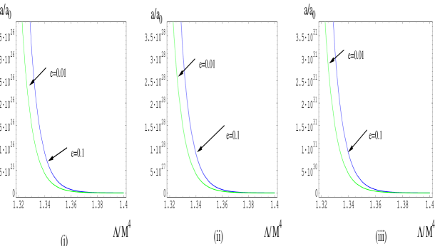
Figure 2: The scale factor as a function of the cosmological constant. Cases $(i)$, $(ii)$, and $(iii)$ refer to the initial conditions $\Lambda_{0}/M^{4}=10^{2}$, $\Lambda_{0}/M^{4}=10^{4}$, and $\Lambda_{0}/M^{4}=10^{7}$, respectively.

According to Fig. 2 there is no strong dependence on the value of the gauge coupling $e$. $a/a_{0}$ has undergone 60 e-foldings, a phenomenological requirement imposed to sufficiently smooth out the inhomogeneities existing prior to inflation. The corresponding points $\Lambda/M^{4}$ turn out to be between 1.34 and 1.44 for the three very different initial conditions! So the (inflationary) regime, where the cosmological constant dominates the energy density, does practically not depend on the initial conditions prescribed at the borderline of applicability of our model. We demand that inflation be terminated at $\Lambda/M^{4}=1.4$ by a transition to the center symmetric regime. Setting $V(|\phi|_{c}^{2})=\Lambda=1.4M^{4}$, yields $N=34$. We will work with this value in the following.

3 Cosmic evolution in thermal equilibrium

3.1 Flat space solution

In this section we evaluate the evolution of the scale factor $a$. For a spatially flat universe ($k=0$) we seek a solution to the Friedmann equation

$$H^{2}(t)\equiv\left(\frac{\dot{a}(t)}{a(t)}\right)^{2}=\frac{8\pi}{3}\,G\,\varepsilon(a)\ .$$ (22)

Far away from the pole in the RHS of eq. (21) we may neglect the constant terms $120\pi^{2}(\kappa_{1}-\kappa_{2})M^{12}$ and can then analytically invert eq. (21), yielding

$$\Lambda=\Lambda_{0}\left(\frac{a}{a_{0}}\right)^{-1}\ .$$ (23)

Inserting this result into the RHS of the Friedmann equation (22) and using eq. (17), we have

$$\left(\frac{\dot{a}}{a}\right)^{2}=\frac{8\pi}{3}\,G\,\left[\frac{\Lambda_{0}^{4}}{160\pi^{2}M^{12}}\left(\frac{a}{a_{0}}\right)^{-4}+\Lambda_{0}\kappa_{1}\left(\frac{a}{a_{0}}\right)^{-1}\right]\ .$$ (24)

For high $T$, where radiation dominates the energy density, we may neglect the term $\propto\left(\frac{a}{a_{0}}\right)^{-1}$ in eq. (24). This yields the usual decelerated expansion due to a relativistic gas

$$\frac{a(t)}{a_{0,r}}=\sqrt{2\alpha_{r}\,(t-t_{0,h})+1}\,,$$ (25)

where

$$\alpha_{r}\equiv\sqrt{\frac{G}{60\pi}}\frac{\Lambda_{0}^{2}}{M^{6}}\ .$$ (26)

There is an intermediate regime, where $M^{4}\gg\Lambda<10M^{4}$ or equivalently, $\frac{M}{2\pi}\ll T<\frac{5M}{\pi}$. The point of equality of radiation and vacuum energy is at $\frac{\Lambda}{M^{4}}\sim 11.6$. For $\Lambda<10M^{4}$ we may neglect the radiation energy still using the scaling law $\Lambda\propto a^{-1}$ obtained for the radiation dominated regime. As far as the duration of this regime is concerned, this approximation is likely to yield an upper bound because it underestimates the value of $\Lambda$ close to the inflationary regime where $\Lambda$ dominates by far the radiation term in the energy density. The solution to eq. (24) then reads

$$\frac{a(t)}{a_{0,rv}}=\left(\frac{\alpha_{rv}}{2}(t-t_{0,rv})+1\right)^{2}\,,$$ (27)

where

$$\alpha_{rv}\equiv\sqrt{\frac{8\pi}{3}G\kappa_{1}\Lambda_{0}}\ .$$ (28)

So there is accelerated expansion.

According to eq. (21) quasi-exponential expansion sets in when $\Lambda$ approaches the zero of $\Lambda^{3}+120\pi^{2}(\kappa_{1}-\kappa_{2})M^{12}$ which blows up the RHS due to the negative exponent $\frac{2\kappa_{1}-3\kappa_{2}}{9(\kappa_{2}-\kappa_{1})}$.

3.2 Decoupling of gravity from inflaton dynamics

We now show that gravity effectively disappears from the Euclidean second-order equations for the inflaton field as a consequence of BPS saturation 2 in the regime of high $T$. According to eqs. (2.1) this would be the case if the ratio

$$R\equiv\left|\frac{3H\,V^{1/2}}{\frac{\partial V}{\partial\phi}}\right|$$ (29)

was much smaller than unity. Neglecting the small vector mass in the radiation dominated era, we have

$$|H_{r}|\sim\sqrt{\frac{8\pi}{3}G\frac{\pi^{2}}{10}T^{4}}\sim\sqrt{\frac{4}{5}}\pi T^{2}/M_{P}\ .$$ (30)

On the other hand, $|V^{1/2}|=\sqrt{2\pi M^{3}T}$. With eq. (30) we then obtain

$$|3H\,V^{1/2}|=3\sqrt{\frac{8}{5}\pi^{3}M^{3}T}\,T^{2}/M_{P}\ .$$ (31)

Substituting the solution of eq. (7) into the derivative of the potential, for we have ($n=1$)

$$\left|\frac{\partial V}{\partial\phi}\right|_{\phi^{(1)}}=(2\pi\,M\,T)^{3/2}\ .$$ (32)

Thus

$$R_{r}\sim\frac{3\sqrt{\frac{8}{5}\pi^{3}M^{3}T}\,T^{2}/M_{P}}{2(2\pi\,M\,T)^{3/2}}=\sqrt{9/5}\frac{T}{M_{P}}\ .$$ (33)

If $T$ is of order $M_{P}$ this ratio is of order unity. So decoupling of gravity becomes effective if the initial temperature is smaller than the Planck mass. Since the dynamics possesses an attractor property in the sub-Planckian regime an implicit assumption for our model to be viable is that Planckian physics drives the universe towards temperatures lower than $M_{P}$.

Let us now consider the ratio $R$ for the inflationary era. There, $|H|$ is determined by the vacuum energy, and we have

$$|H_{i}|\sim\sqrt{\frac{8\pi}{3}G2\pi M^{3}T}\sim\sqrt{16\pi}M^{3/2}T^{1/2}/M_{P}\ .$$ (34)

So together with eqs. (31,32) and $T\sim M/2\pi$ we obtain

$$R_{i}\sim 2\sqrt{18}\frac{M}{M_{P}}<10^{-3}\$$ (35)

for $M$ being smaller than the GUT scale $\sim 10^{16}$ GeV. Thus gravity effectively decouples from the inflaton dynamics during and well before inflation.

3.3 A numerical example

We are now in a position to demonstrate a particular inflationary scenario. Let us assume that the Hubble parameter $H$ is quasiconstant along a time interval $\Delta t_{i}\sim 10^{-30}\,$s. Imposing that inflation should at least generate 60 e-foldings,

$$\Delta t_{i}H=60=10^{-30}\times\frac{3}{2}\times 10^{24}\,\mbox{GeV}^{-2}\times 2.4\times 10^{-19}\times M^{2}\ ,$$ (36)

we obtain $M\sim 1.3\times 10^{13}\,$GeV. This is considerably lower than the scale of grand unification $\sim 10^{16}\,$GeV, and hence the density of topological defects potentially arising during GUT phase transitions does get diluted to immeasurability during inflation. We use this value for $M$ to estimate the time scales of the two regimes preceding inflation. For definiteness let us assume Planck scale initial conditions $\Lambda_{0}=10^{7}\,M^{4}$. With $M=1.3\times 10^{13}\,$GeV this yields

$$\alpha_{r}=\sqrt{\frac{G}{60\pi}}\frac{\Lambda_{0}^{2}}{M^{6}}\sim 1.01\times 10^{20}\,\mbox{GeV}\ .$$ (37)

According to eq. (25) the time interval $\Delta t_{r}$ belonging to the radiation dominated phase is given as

$$\Delta t_{r}=\frac{1}{2\alpha_{r}}\left[\left(\frac{a_{r}}{a_{0,r}}\right)^{2}-1\right]\ ,$$ (38)

where $a_{r}$ and $a_{0,r}$ denote the scale factors at the end and the beginning of this regime, respectively. From a numerical evaluation of eq. (21) we obtain $\frac{a_{r}}{a_{0,r}}\sim 10^{6}$ for $\Lambda\sim 10\,M^{4}$ marking the end of the epoch of radiation domination. Using this together with eqs. (38,37), we have

$$\Delta t_{r}\sim 3.3\times 10^{-33}\,\mbox{s}\ .$$ (39)

So on a logarithmic scale the radiation dominated epoch before inflation lasted rather long.

Let us now define the epoch of spontaneous gauge symmetry breaking being driven by a mixture of radiation and vacuum energy. Evolving from $\Lambda=10\,M^{4}$, where for Planckian initial conditions we had ${a_{r}}/a_{0,r}\sim 10^{6}$, we define the start of inflation by $\Lambda=2\,M^{4}$ corresponding to $a/a_{0,r}\sim 10^{13}$. This yields ${a_{rv}}/a_{0,rv}\sim 10^{7}$. The expansion parameter $\alpha_{rv}$ can be computed as

$$\alpha_{rv}=\sqrt{\frac{8\pi G}{3}\Lambda_{0}}\sim 1.3\times 10^{8}\,\mbox{GeV}\ .$$ (40)

Solving eq. (27) for $\Delta t_{rv}$, we obtain

$$\Delta t_{rv}=\frac{2}{\alpha_{rv}}\,\left(\sqrt{\frac{a_{rv}}{a_{0,rv}}}-1\right)\ .$$ (41)

Combining eqs. (40,41) and using ${a_{rv}}/a_{0,rv}\sim 10^{7}$, we have

$$\Delta t_{rv}\sim 3\times 10^{-29}\,\mbox{s}\ .$$ (42)

This is a little more but rather close to the assumed duration of inflation of $\Delta t_{i}\sim 10^{-30}\,$s. However, as was argued above, this must be an artifact of the approximation made leading to eq. (41).

We now can compare the results obtained in the above, semi-analytic fashion with a numerical result. Fig. 3 shows the computed time evolution of the scale factor. It is seen that the radiation approximation worked well. The numerically evolution of $a$ in the $rv$ regime, however, is stronger than our analytical estimate.

Figure 3: Comparison of semi-analytical approximation and numerical results for the regimes of radiation ($i$) and of radiation-vacuum mixture ($ii$) in a spatially flat universe. The evolution of the scale factor from Planckian initial conditions to inflationary cosmology is shown in ($iii$).

3.4 Closed universes need not collapse.

Here we address the fate of a closed universe ($k=+1$ in eq. (43)). In the case of a closed or an open universe the square of the Hubble parameter $H$ contains an extra term and is given as

$$H^{2}=\frac{8\pi G}{3}\left(\frac{\Lambda^{4}}{160\pi^{2}M^{12}}+\kappa_{1}\Lambda-\frac{3k}{8\pi Ga^{2}(t)}\right)\ .$$ (43)

For a closed universe not to collapse in the course of its evolution the RHS of eq. (43) must remain positive. Using radiation scaling $\Lambda=\Lambda_{0}\frac{a_{0,r}}{a}$, $G^{-1}=M_{P}^{2}$, and the following relations valid for the Planckian regime

$$\Lambda_{0}=2\pi T_{0}M^{3}=2\pi M_{P}M^{3}\,,\ \ \ \ \ \ M\sim 10^{-6}M_{P}\ ,$$ (44)

we can cast this condition into the form

$$f(x)\equiv\sqrt{\frac{4}{15}\pi^{3}x^{2}+\frac{16}{3}\pi^{2}\kappa_{1}\times 10^{-18}\frac{1}{x}}>(a_{0,r}M_{P})^{-1}\ .$$ (45)

Thereby, we have defined $0<x\equiv\frac{a_{0,r}}{a}\leq 1$. Eq. (45) yields a lower bound on the radius $a_{0}$ of the universe at Planckian energy density provided that radiation scaling is applicable. For estimation purposes we can safely set $\kappa_{1}=1$. The only extremum of the function $f(x)$ in $0\leq x\leq 1$ is a minimum at $x_{m}\sim 1.5\times 10^{-6}$. This corresponds to $f(x_{m})\sim 7.3\times 10^{-6}$ yielding the following lower bound for $a_{0}$

$$a_{0,r}>\frac{1}{7.3}\times 10^{6}M_{P}^{-1}\sim 10^{5}M_{P}^{-1}\ .$$ (46)

Note that the above scaling assumption for $\Lambda$ is justified a posteriori due to the results of the last section stating that at $x_{m}\sim 1.5\times 10^{-6}$ radiation scaling is an excellent approximation. Thus, we have proved that closed universes do not collapse in the course of their evolution provided their radius $a_{0,r}$ at Planckian density is larger than some critical value. Fig. 4 shows numerical evolutions for open, flat, and closed universes. Thereby, the initial radius $a_{0,r}=1/8.65\times 10^{6}M_{P}^{-1}$ has been chosen very close to the critical value. The reader may object to the large hierarchy of $\sim 10^{5}$ between $a^{-1}_{0,h}$ and $M_{P}$. This hierarchy has its origin in the theory of matter and that of gravity being governed by the hierarchical mass scales $M$ and $M_{P}$, respectively, at the very regime of separation of the two theories. Only a consistent unified theory of gravity and matter can explain this fact. Needless to say, such a theory does not yet exist.

We stress at this point that in a conventional scenario, where the matter of the universe close to Planckian density is composed of radiation and a $T$ independent $\Lambda$, there always will be a collapse. This is due to the second term under the square root in eq. (45) being a constant. The global minimum of the corresponding function $f_{c}(x)$ then is at $x=0$, which invalidates the derivation of the inequality corresponding to eq. (45).

Figure 4: Evolution of open, flat and closed universes. We have set $a_{0,r}=1/8.65\times 10^{6}M_{P}^{-1}$ which is very near to the critical radius for a closed universe.

4 The universe after inflation

4.1 Termination of inflation and reheating

Quasi-exponential expansion is terminated at the point where the inflaton amplitude starts to fluctuate putting an end to vacuum dominance. In our model this effect sets in at $|\phi|=|\phi|_{c}$. Even the solutions to the Euclidean mean field equations yield a time dependent inflaton amplitude indicating the breakdown of thermal equilibrium. Therefore, the dynamics can not be treated in Euclidean signature anymore. On the other hand, the spontaneously broken gauge symmetry is reduced to a spontaneously broken $Z_{N+1}$ symmetry. Thus, gauge bosons cease to get emitted from the vacuum. The gauge theory is reduced to a theory of a complex scalar field moving mainly along one of the unit root directions and hence to a good approximation can be chosen real. To give an estimate on the number of Hubble times, which the subsequent regimes of tachyonic preheating and reheating last, we consider spatially homogeneous fluctuations obeying to linear order

$$\ddot{\delta\phi}+3H\dot{\delta\phi}-m^{2}(\phi_{0})\delta\phi=0\,,$$ (47)

where $m^{2}\equiv\left.\frac{\partial^{2}V}{\partial\phi^{2}}\right|_{\phi=\phi_{0}}$. The mean field $\phi_{0}$ denotes a solution to the full equation of motion. Therefore, $\delta\phi\sim e^{mt}$. Numerically, $m$ is of the order of several $M$ during tachyonic preheating. On the other hand, the Hubble parameter $H$, which can be taken inflation valued, is $H\sim\frac{M}{M_{P}}M\sim 10^{-6}M$. If we do not allow for a fine-tuning of the initial conditions for $\delta\phi$ the typical time interval $\Delta t_{tac}$ the system is in the tachyonic regime is about $10^{-6}$ inflationary Hubble times. During the subsequent regime of reheating (positive mass squared) $\phi$ performs damped oscillations about its vacuum value $\phi=M$. If there were only a few oscillations then this regime would last again only about $10^{-6}$ Hubble times since the frequency of oscillation should be comparable to the mass of excitations $NM=34\,M$ [14]. Let us compare this picture with numerical simulations of similar situations not assuming spatial homogeneity of $\phi$.

On the lattice it was found recently [25, 26, 27] (and references therein) that the tachyonic instability of the field $\phi$ staying close to the symmetry conserving maximum of its potential at inflation converts most of the inflation valued $\Lambda$ into matter due to tachyonic preheating. One must distinguish between $\phi$ independent and $\phi$ dependent curvature at this maximum. In the former case the energy release during tachyonic preheating was found to be so efficient that a single oscillation of the inflaton field relaxes it to the minimum of the potential. In order to arrive at this result, a quantum mechanical dispersion of the field amplitude was assumed and evolved. The occupation numbers of fluctuations at low momenta grow exponentially in the early stage of the process. If the potential possesses a discrete symmetry then at later stages of the evolution this growth spreads to higher momenta due to the formation of domain walls and classical wave collisions. It was stressed in refs. [26, 27] that initially large domains grow by “eating” smaller domains so that the field distribution becomes completely asymmetric after some finite time being bounded roughly by the mass scales of the potential. This is important since the phenomenon of cannibalizing domains excludes domain walls within today’s horizon being dangerous for present day cosmology. Our inflaton potential is qualitatively similar to that of the Coleman-Weinberg model investigated in ref. [26]. Likewise, the $Z_{2}$ symmetric potential of this model possesses a $\phi$ dependent curvature which vanishes at the initial point $\phi_{i}$ of the process. The following results were obtained in ref. [26]: Due to vanishing initial curvature individual fluctuations are quasistable so tachyonic growth does not happen. However, there is instanton mediated quantum tunneling towards the regime where perturbative, tachyonic fluctuations drive the transition along the lines of what was said above. Therefore, domain growth by “eating” should proceed in analogy to pure tachyonic preheating once the transition to the regime of tachyonic fluctuations is achieved through nonperturbative effects.

So qualitatively we obtain the same estimate for the duration of the regimes of tachyonic preheating and reheating. On the other hand, we may easily estimate how long a co-moving mode, which exits the horizon during inflation, is outside the horizon after inflation: The condition is

$$H=\left.(Ha)\right|_{entry}\frac{1}{a_{0}}=\left.(Ha)\right|_{entry}\frac{1}{a^{i}_{0}}\frac{a^{i}_{0}}{a_{0}}\ ,$$ (48)

where $a_{0}$ and $a^{i}_{0}$ are the scale factors at horizon exit and end of inflation, respectively, and $H$ is the Hubble parameter at inflation. We write $\frac{a^{i}_{0}}{a_{0}}=\mbox{e}^{n}$. For the radiation dominated epoch after reheating we obtain

$$\left.H\right|_{entry}=\frac{2M^{2}\sqrt{\frac{8\pi}{3}G}}{2\sqrt{\frac{8\pi}{3}G}M^{2}(t-t_{0}^{i})+1}\ ,$$ (49)

where $t_{0}^{i}$ is the end of inflation. From eqs. (48,49) we obtain

$$t-t_{0}^{i}=\frac{1}{2}(4\mbox{e}^{2n}-1)H^{-1}\sim H^{-1}\ .$$ (50)

This is to be contrasted with the time scale $\sim 10^{-6}H^{-1}$ tachyonic preheating and reheating takes. Thus it is appropriate to say that termination of inflation and reheating proceed instantaneously.

4.2 Adiabatic density perturbations due to the inflaton field?

The usual procedure to take into account adiabatic density perturbations originating from the inflaton field is the following: In the presence of a reservoir quantum fluctuations of the field $\phi$ are composed of vacuum fluctuations, which are always renormalized away [5], and excitations of momentum $k$. A mode with co-moving momentum $k_{c}=\frac{a}{a_{0}}k$ exits the horizon during inflation at $\frac{a}{a_{0}}H=k_{c}$. If we have $m\ll H$ for the mass $m$ of this mode and if there is a sufficient amount of inflation after horizon-exit the quantum fluctuation is frozen into a classical, Gaussian perturbation with the root of the mean-square given in the massless limit as [28]

$$\delta\phi(k)\equiv\frac{H}{2\pi}\ ,$$ (51)

where $H$ is the (quasiconstant) Hubble parameter at inflation. If the particular mode enters the horizon well after the reheating epoch its corresponding density perturbation becomes the seed for a curvature perturbation. This, in turn, is responsible for structure formation at the associated physical length scale [28]. The density contrast $\frac{\delta\rho(k)}{\rho}$ during inflation can be estimated as [5]

$$\frac{\delta\rho(k)}{\rho}=\frac{\delta V(\phi(k))}{V(\phi)}\ .$$ (52)

Due to our thermodynamical approach the situation is rather different here: The condition $m\ll H$ for slow-roll of the field $\phi$ in a treatment based on Minkowskian signature is not satisfied. On the contrary, we have $m\sim 10^{6}H\gg H$. Nevertheless, during inflation $|\phi|$ rolls very slowly due to a very slowly varying temperature.

Since the energy density of the radiation is suppressed by a factor of about $(2\pi)^{-4}$ as compared to the vacuum energy density we do expect the density fluctuations in the radiation part to be of no significance. Let us therefore focus on scalar fluctuations. How relevant are these fluctuations during inflation which is characterized by a temperature $T_{i}\sim\frac{M}{2\pi}$? The occupation number is of the Bose type

$$n^{s}_{B}(k)=\frac{1}{\exp\left[\frac{\sqrt{k^{2}+m_{i}^{2}}}{T}\right]-1}\ ,$$ (53)

where $m_{i}$ denotes the mass of scalar excitations during inflation. We have

$$m_{i}\sim\sqrt{6}\,\frac{M^{3}}{\phi_{c}^{2}}\sim\sqrt{6}\,M\ .$$ (54)

An upper bound for $n^{s}_{B}(k)$ during the part of inflation, where $m_{i}$ can be estimated according to eq. (54), is

$$n^{s}_{B}(k)\leq\frac{1}{\exp\left[\frac{m_{i}}{T_{i}}\right]-1}\sim 2\times 10^{-7}\ .$$ (55)

Hence, there are practically no fluctuations of $\phi$. However, shortly before inflation terminates (${\partial_{|\phi|}^{2}V}=0$) the mass of fluctuations reduces down to values comparable with $T_{i}$, and excitations are possible. To estimate the magnitude of field perturbations possibly seeding the formation of large-scale structure following [5] we write

$$\left\langle(\delta\phi)^{2}\right\rangle=\frac{1}{(2\pi)^{3}}\int\frac{d^{3}k}{\sqrt{k^{2}+m^{2}}}n(k)\ ,$$ (56)

where $n(k)$ denotes the occupation number of the state with spatial momentum $k$, in our case $n=n_{B}$. Eq. (56) is to be interpreted as a weighted sum over all excitable modes that may leave the horizon before inflation ends. If we assume that the mass $m$ remains roughly constant at value $T_{i}$ during this last stage of inflation an evaluation of $n_{B}$ at horizon exit $k=H$ yields $n_{B}\sim 1/2$. Moreover, assuming that the universe expanded $e^{n}$ times from the first exit of an excited mode to the end of inflation, we obtain the following estimate

$$\left\langle(\delta\phi)^{2}\right\rangle=\frac{1}{4\pi^{2}m}\int_{a^{-1}H}^{H}dkk^{2}=\frac{1}{4\pi^{2}}\left[1-e^{-3n}\right]\frac{H^{3}}{m}<\frac{1}{4\pi^{2}}\frac{H^{3}}{m}\ .$$ (57)

An upper bound for the corresponding density contrast is

$$\frac{\delta T}{T}\sim\frac{\delta\rho}{\rho}\equiv\left.\frac{\partial V/\partial\phi}{V}\,\delta{\phi}\right|_{\phi=\phi_{c}}\sim 10^{-9}\ .$$ (58)

This is much too low to explain the measured anisotropy $\frac{\delta T}{T}\sim 10^{-5}$ of the CMBR. Therefore, the required density perturbations do not originate from the fluctuations of the inflaton field in our model. Recently, it was proposed in [7] that the spatial curvature perturbations required for the formation of the large scale structure can originate from a light scalar field not driving inflation. Our model has to be supplemented with such a mechanism for the generation of density perturbations. However, it is conveivable that a consensate of composite bosons originating from fundamentally charged matter may play the role of this light scalar field. We hope to address this issue in a forthcoming publication.

There is a final, rather important observation concerning isothermal density fluctuations. These fluctuations are associated with a much smaller mass scale than the field driving and terminating inflation. Typical candidates for the generation of isothermal fluctuations are the Goldstone modes of the spontaneous breakdown of a continuous, global symmetry [29]. Due to the assumption of pure underlying gauge dynamics we only have a spontaneous breakdown of a $Z_{N+1}$ symmetry during tachyonic preheating. However, (a) this symmetry originated from a gauge symmetry [16], and (b), it is not continuous. Therefore, Goldstone modes associated with the termination mechanism of inflation do not exist in our minimal model.

5 Summary and outlook

We proposed a model for cosmic inflation based on the thermal equilibrium dynamics of a higgsed $U(1)$ gauge theory which, in turn, represents an effective description of underlying $SU(N+1)$ pure gauge dynamics. This was motivated by a possible description of fundamental, non-Abelian, and unhiggsed gauge theories in terms of Abelian Higgs models [10, 14]. Identifying the Higgs field with the inflaton, we constructed the corresponding scalar potential such that the theory admits BPS saturated periodic inflaton solutions. The dynamics following from this potential represents a concrete realization of Krauss’ and Wilczek’s proposal that gauge symmetries masquerade as discrete subgroups when tested with low energies [16]. Solving the vacuum gauge field equation in this background according to a Born-Oppenheimer approximation, implied a vanishing, gauge invariant kinetic term in the action. Therefore, we obtained a temperature dependent cosmological constant upon trivial analytical continuation to Minkowskian signature as the sole contribution from the scalar sector to the total stress energy of the universe. The Friedmann equations adapted to this set-up yielded cosmic inflation at a scale being independent of initial conditions. The $T$ dependence of $\Lambda$ prevents closed universes from collapsing provided the initial radius is large enough. We considered the mechanisms responsible for a termination of inflation and thereby observed that the point at which the gauge symmetry starts to masquerade as a $Z_{N+1}$ symmetry coincides with a noticeable violation of thermal equilibrium. It is stressed at this point that the estimate for the maximal number of e-foldings during thermal inflation as it was performed in ref. [9] does not apply to our model. In [9] it was assumed that temperature decreases as $\sim\exp[-Ht]$. On the contrary, temperature remains constant during inflation in our approach. This is a direct consequence of the vacuum itself carrying a nonvanishing heat capacity. Recall that the determination of the scale $M\sim 10^{13}$ GeV in section 3.3 originated from demanding that inflation is to generate about 60 e-foldings at $t\sim 10^{-30}$ s. Towards the end of inflation, excitations become first massless and later tachyonic. The conventional mechanism for the generation of density perturbations from quantum fluctuations of the inflaton field during inflation does not apply to our model. The reason is that the mass of scalar excitations during the bulk of inflation is much larger than the Hubble parameter which is in contrast to the usual slow-roll paradigm. However, one may invoke the recently advocated curvaton [7] to generate density perturbations independently from the inflaton dynamics.

The rapid decay of the old vacuum is accompanied by the generation of new particles whose dynamics is subject to the prevailing $Z_{N+1}$ symmetry. This symmetry strongly suppresses the decay of the old vector bosons [16], [17]. Hence, these particles of mass $10^{11}$ – $10^{13}$ GeV could survive to the present. They contribute to the dark matter content and originate ultra-high energy cosmic rays beyond the Greisen-Zatsepin-Kuzmin bound. This possibility was first discussed in ref. [30]. Due to their high mass the relic vector bosons may also function as considerable dark matter sources.

We speculate that the cosmologically relevant (equilibrium) dynamics following the termination of inflation and particle creation is effectively described by a member of the same class of Abelian Higgs models labeled by the parameters $(e,M,N)$. The mass scale involved would be lower and therefore a sequence of milder and milder inflations is induced. It is tempting to interpret the emission of the CMBR as the particle creation stage following the last inflation. The vacuum structure being established would then be associated with the electromagnetic interaction. With $\Omega_{\Lambda}\sim 0.7$ one would expect that the corresponding inflaton field $\phi_{em}$ was close to the inflationary regime. Therefore, one could estimate the scale $M_{em}$ by using the limiting formula $|\phi_{em}|\sim M_{em}$ and $T\sim\frac{M_{em}}{2\pi}$. However, there is at least one good reason to reject this possibility: A bound on the photon mass is $m_{\gamma}<10^{-16}\,$eV [32]. Using the electromagnetic coupling $\alpha_{em}=\frac{e_{em}^{2}}{4\pi}=\frac{1}{137}$, one obtains from $m_{\gamma}=e_{em}|\phi_{em}|\sim e_{em}M$ that $M_{em}\;^{<}\!\!\!\!{}_{\sim}\;3\times 10^{-16}\,$eV. Therefore, the energy density attributed to this vacuum is $\Lambda_{em}\sim M^{4}\sim 30\times 10^{-64}\,(\mbox{eV})^{4}$. On the other hand, the temperature of the CMBR is $\sim 3\,\mbox{K}=0.25\times 10^{-3}\,$eV. This corresponds to $M_{em}\sim 2\pi T\sim 1.6\times 10^{-3}\,$eV which is in stark contradiction to the value deduced from the photon mass bound. So if the present accelerated expansion is again driven by a higgsed, Abelian gauge theory it probably has nothing to do with the interactions of the standard model of particle theory. This, however, leaves us with an exciting perspective regarding today’s measured ratio of $\Omega_{\Lambda}$ and $\Omega_{\rm{dark\;matter}}$. Assuming that an otherwise undetected Abelian Higgs model drives today’s accelerated expansion, our scenario easily accommodates this ratio.

References

- [1] A.H. Guth, Phys. Rev. D23, 347 (1981).
-
[2]
A.D. Linde, Phys. Lett. B108, 389 (1982).
A. Albrecht and P.J. Steinhardt, Phys. Rev. Lett. 48, 1220 (1982).
A.H. Guth and P.J. Steinhardt, Sci. Am., May 1984, p. 90. - [3] A.D. Linde, Rep. Prog. Phys. 47, 925 (1984).
- [4] A.D. Linde, hep-th/0110195.
- [5] A.D. Linde, Inflation and Quantum Cosmology, Academic Press, Inc., Harcourt Brace Jovanovich, Publishers (1990), and references therein.
- [6] C. Armendariz-Picon and V.F. Mukhanov, Int. J. Theor. Phys. 39,1877 (2000).
-
[7]
D.H. Lyth and D. Wands, Phys. Lett. B524, (2002) 5, hep-ph/0110002.
T. Moroi and T. Takahashi, Phys. Lett. B522, (2001) 215, hep-ph/0110096. - [8] L. Randall and S. Thomas, Nucl. Phys. B449, 229 (1995), hep-ph/9407248.
- [9] D.H. Lyth and E.D. Stewart, Phys. Rev. D53, 1784 (1996).
-
[10]
S. Mandelstam, Phys. Rep. C23, 245 (1976).
G. ’t Hooft, Nucl. Phys. B190, 455 (1981).
T. Suzuki, Prog. Theor. Phys. 80, 929 (1988); 81, 752 (1989).
S. Maedan and T. Suzuki, Prog. Theor. Phys. 81, 229 (1989).
H. Ichie, H. Suganuma and H. Toki, Phys. Rev. D 52, 2944 (1995).
M.N. Chernodub, F.V. Gubarev, M.I. Polikarpov, V.I. Zakharov, Nucl. Phys. B600,163 (2001), hep-th/0010265. - [11] G. Mack and E. Pietarinen, Nucl. Phys. B205, 141 (1982).
-
[12]
L. Del Debbio, M. Faber, J. Greensite, and S. Olejnik, Phys. Rev. D55, 2298 (1997).
P. de Forcrand and M. D’Elia, Phys. Rev. Lett. 82, 4582 (1999). -
[13]
M. Engelhardt and H. Reinhardt, Nucl. Phys. 585, 591 (2000), hep-lat/9912003.
M. Engelhardt, Nucl. Phys. B585, 614 (2000), hep-lat/0004013.
M. Engelhardt, hep-lat/0204002. - [14] R. Hofmann, hep-ph/0201073, to app. in Phys. Rev. D.
-
[15]
E.B. Bogomolny, Sov. J. Nucl. Phys. 24, 449 (1976).
M.K. Prasad and C.M. Sommerfield, Phys. Rev. Lett. 35, 760 (1975). - [16] L.M. Krauss and F. Wilczek, Phys. Rev. Lett. 62, 1221 (1989).
-
[17]
K. Hamaguchi, Y. Nomura, and T. Yanagida, Phys. Rev. D58, 103503 (1998), hep-ph/9805346.
K. Hamaguchi and Y. Nomura, Phys. Rev. D59, 063507 (1999), hep-ph/9809426.
J.D. Cohn and E.D. Stewart, Phys. Lett. B475, 231 (2000), hep-ph/0001333.
J.D. Cohn and E.D. Stewart, Phys. Rev. D63, 083519 (2001), hep-ph/0002214. - [18] R. Hofmann, Phys. Rev. D62, 105021 (2000), hep-ph/0006163, Erratum-ibid. D63, 049901 (2001).
- [19] G. Dvali and M. Shifman, Phys. Lett. B454, (1999) 277.
-
[20]
T. C. Kraan and P. van Baal, Nucl. Phys. A642, 299 (1998), hep-th/9805201.
T. C. Kraan and P. van Baal, Phys. Lett. B435, 389 (1998), hep-th/9806034.
M. Garcia Perez, A. Gonzalez-Arroyo, A. Montero, and P. van Baal, JHEP 06, 001 (1999), hep-lat/9903022. - [21] S. Weinberg, Gravitation and Cosmology, John Wiley & Sons, Inc. (1972).
- [22] R. Hofmann, Phys. Rev. D62, 065012 (2000), hep-th/0004178.
-
[23]
A. Sornborger and M. Parry, Phys. Rev. Lett. 83, 666 (1999), hep-ph/9811520.
A. Sornborger and M. Parry, Phys. Rev. D62, 083511 (2000), hep-ph/0004230. - [24] I. Dymnikova and M. Khlopov, Eur. Phys. J. C20, 139 (2001).
- [25] J.G. Garcia-Bellido and E. Ruiz Morales, hep-ph/0109230.
- [26] G.N. Felder, L. Kofman, A.D. Linde, hep-th/0106179.
- [27] M.F. Parry and A.T. Sornborger, Phys. Rev. D60, 103504 (1999), hep-ph/9805211.
- [28] A.R Liddle and D.H. Lyth, Cosmological Inflation and Large Scale Structure, Cambridge University Press (2000).
-
[29]
M. Bucher and Y. Zhu, Phys. Rev. D55, 7415 (1997), astro-ph/9610223.
A. Dolgov and K. Freese, Phys. Rev. D51, 2693 (1995), hep-ph/9410346.
K. Freese, Phys. Rev. D50, 7731 (1994), astro-ph/9405045. -
[30]
V. Berezinsky, M. Kachelriess, A. Vilenkin, Phys. Rev. Lett. 79, 4302 (1997), astro-ph/9708217.
V.A. Kuzmin and V.A. Rubakov, Phys. Atom. Nucl. 61, 1028 (1998), astro-ph/9709187. -
[31]
A.G. Riess et al., Astron. J. 116, 1009 (1998), astro-ph/9805201.
S. Perlmutter et al., Astrophys. J. 517, 565 (1998), astro-ph/9812133. - [32] D.E. Groom et al., Eur. Phys. J. C15, 1 (2000).