Modern Physics Letters A,
c  World Scientific Publishing Company

1

MASS EFFECTS ON THE NUCLEON SEA STRUCTURE FUNCTIONS

Sun Myong Kim

Department of Liberal Arts and Sciences

Halla University

WonJu, Kangwondo 220-840, Korea

Received (received date)
Revised (revised date)

Nucleon sea structure functions are studied using Dokshitzer-Gribov-Lipatov-Altarelli-Parisi (DGLAP) equations with the massive gluon-quark splitting kernels for strange and charm quarks, the massless gluon-quark splitting kernels for up and down quarks, and the massless kernels for all other splitting parts. The $SU(2)_{f}$ flavor symmetry for two light quarks, ‘up’ and ‘down’, is assumed. Glück-Reya-Vogt(GRV) and Martin-Roberts-Stirling(MRS) sets are chosen to be the base structure functions at $Q_{0}^{2}=3$ GeV². We evolve the sea structure functions from $Q_{0}^{2}=3$ GeV² to $Q^{2}=50$ GeV² using the base structure function sets and DGLAP equations. Some (about 10%) enhancement is found in the strange quark distribution functions at low $x(<0.1)$ in leading order of the DGLAP equations compared to results direclty from those structure function sets at the the value of $Q^{2}=50$ GeV². We provide the value of $\kappa$ and also show the behavior of $\kappa(x)=2s(x)/(\bar{u}(x)+\bar{d}(x))$ after the evolution of structure functions.

The nucleon structure function at low $x$ ^? and at high $x$ may bare non-perturbative effects. However, we can still investigate the structure function at not so low $x(\simeq 10^{-1}-10^{-3})$ with perturbative QCD. At this low $x$, sea quarks and gluons play important roles in QCD processes. Disagreements between theoretical and experimental results in various sum rules suggest the necessity of more improved theoretical analysis in nucleon structure functions, especially, in sea quark distribution functions in this region of $x$.

The traditional analysis of sea quark distribution functions for three light quarks (up, down, and strange) has been based either on the $SU(3)_{f}$ flavor symmetry or on an ad hoc choice of $s(x)={1\over 2}\bar{u}(x)={1\over 2}\bar{d}(x)$ (or $s(x)=\bar{u}(x)=\bar{d}(x)$). Now, we are able to probe these sea structure functions at low $x$ (up to $\simeq 10^{-4}$) and high $Q^{2}$ with better statistics. The validity of the $SU(3)_{f}$ symmetry assumption and the ad hoc choice of the strange quark structure function has been at stake ^?.

Although we believe that there are many signatures that treating strange quark on an equal footing as other two light quarks is not correct, it is not clear what physics should be applied and how to implement it to differentiate its roles in the structure functions. In this letter, we treat strange and charm quarks massive. The mass effect is one of several possible factors affecting the structure functions such as the non-perturbative QCD effect and the different Pauli exclusion effect for $\bar{u}$, $\bar{d}$, and $s$ quarks which should be taken into account due to different numbers of valence $u$ and $d$ quarks in the proton. On this principle, however, there have been speculations that the effects may be marginal ^?.

To observe sea quarks in the nucleon (proton), we consider the process of the deep inelastic scattering of charged lepton off the nucleon. However, we do not consider the charged weak-current process for simplicity and clarity ^?. To obtain sea structure functions, we use massive kernels ^? for strange and charm quarks in gluon-quark splitting kernels in Dokshitzer-Gribov-Lipatov-Altarelli-Parisi (DGLAP) equations ^? while we keep the $SU(2)_{f}$ flavor symmetry for two light quarks, up and down, by taking massless kernels for the splitting function. We also keep massless kernels for all other splitting parts. Unlike our earlier work ^? where we used an approximate expression for DGLAP equations for the quark structure functions, we solve numerically and explicitly the DGLAP equations for the relevant structure functions in leading order of $\alpha_{s}$.

The DGLAP equations and the corresponding kernels to the quark and gluon distribution functions are given below.

$${dq_{i}(x,Q^{2})\over d\ln Q^{2}} = {\alpha_{s}(Q^{2})\over 2\pi}\int_{x}^{1}{dz\over z}\big{[}P_{qq}(x/z)~{}q_{i}(z,Q^{2})+P_{qg}(x/z)~{}g(z,Q^{2})\big{]},$$ (1)

$${dg(x,Q^{2})\over d\ln Q^{2}} = {\alpha_{s}(Q^{2})\over 2\pi}\int_{x}^{1}{dz\over z}\big{[}\sum_{i}^{N_{f}}P_{gq}(x/z)~{}q_{i}(z,Q^{2})+~{}P_{gg}(x/z)~{}g(z,Q^{2})\big{]}.$$ (2)

Where, the splitting kernels are defined as

$$P_{qq}(z) = {4\over 3}{1+z^{2}\over(1-z)_{+}}+2\delta(1-z),$$ (3)

$$P_{qg}(z) = {1\over 2}\big{[}z^{2}+(1+z)^{2}\big{]},$$ (4)

$$P^{m}_{qg}(z) = {1\over v}\bigg{[}{z^{2}+(1+z)^{2}\over 2}+{m_{q}^{2}\over Q^{2}}{z(3-4z)\over 1-z}-16{m_{q}^{4}\over Q^{4}}z^{2}\bigg{]}$$ (7)

$$-\bigg{[}2{m_{q}^{2}\over Q^{2}}z(1-3z)-8{m_{q}^{4}\over Q^{4}}z^{2}\bigg{]}\ln\bigg{(}{1+v\over 1-v}\bigg{)},$$

$${\rm where,~{}~{}~{}}v^{2}=1-{4m_{q}^{2}\over Q^{2}}{z\over 1-z},$$

$$P_{gq}(z) = {4\over 3}{1+(1-z)^{2}\over z},$$ (8)

$$P_{gg}(z) = 6\bigg{[}{z\over(1-z)_{+}}+{1-z\over z}+z(1-z)+\big{(}{11\over 12}-{f\over 18}\big{)}\delta(1-z)\bigg{]}.\$$ (9)

Where, $q_{i}$ is the quark distribution function for the corresponding flavor ‘$i$’ and ‘$i$’ covers all possible quark and anti-quark flavors. We include only four quark flavors in this numerical calculation by excluding bottom and top quarks for simplicity. The inclusion of these quraks is straight forward but it will not change our current result noticably.

We use massless kernels, $P_{qq}$, $P_{gg}$, $P_{gq}$ in the calculation. For the gluon-quark splitting kernel, however, we use the massive kernel $P^{m}_{qg}$ for strange and charm quarks while we use the massless kernel $P_{qg}$ for up and down quarks. Note that $P^{m}_{qg}\rightarrow P_{qg}$ as $m_{q}\rightarrow 0$ (or $m_{q}^{2}/Q^{2}\rightarrow 0$). Also, the terms in the massive kernel $P^{m}_{qg}$ have the power ($m_{q}^{2}/Q^{2}$) suppression like the ones appearing in higher twist calculation. We choose the massive kernel, $P^{m}_{qg}$, for heavy flavors only in the $g\rightarrow q$ splitting part since $g(x,Q^{2})$ is the most dominant structure functions at low $x$. The ‘+’ prescription is defined in standard way,

$$\int_{0}^{1}dz{f(z)\over(1-z)_{+}}\equiv\int_{0}^{1}dz{f(z)-f(1)\over 1-z}.$$ (10)

To solve numerically the DGLAP integro-differentioal equations for the quarks and gluons, we take the advantage of the differential form of the equations. We start the evolution of the structure functions at $t=t_{0}$ and plug them into the original equations at next $t=t_{0}+\Delta t$. Then, iterate them until we get the desired value of $t(Q^{2})$. Where $t=\ln(Q^{2}/\overline{\Lambda}^{2})$.

$${dq_{i}(x,t)\over dt} = {\alpha_{s}(t)\over 2\pi}\int_{x}^{1}{dz\over z}\bigg{\{}P_{qq}(x/z)\big{[}~{}q_{i}(z,t_{0})+{dq_{i}(z,t)\over dt}\Big{|}_{t=t_{0}}\Delta t~{}\big{]}$$

$$\qquad\qquad~{}~{}+~{}P_{qg}(x/z)\big{[}~{}g(z,t_{0})+{dg(z,t)\over dt}\Big{|}_{t=t_{0}}\Delta t~{}\big{]}\bigg{\}},$$

$${dg(x,t)\over dt} = {\alpha_{s}(t)\over 2\pi}\int_{x}^{1}{dz\over z}\bigg{\{}\sum_{i}^{N_{f}}P_{gq}(x/z)\big{[}~{}q_{i}(z,t_{0})+{dq_{i}(z,t)\over dt}\Big{|}_{t=t_{0}}\Delta t~{}\big{]}$$ (13)

$$\qquad\qquad~{}~{}+~{}P_{gg}(x/z)\big{[}~{}g(z,t_{0})+{dg(z,t)\over dt}\Big{|}_{t=t_{0}}\Delta t~{}\big{]}\bigg{\}}.$$

As the base structure functions we take two typical structure function sets (GRV and MRS) ^?, ^? at the initial value, $Q^{2}_{0}$ and then, evolve the functions using the above DGLAP equations to the given value, $Q^{2}$. The Glück-Reya-Vogt(GRV) set contains structure functions in first two lowest orders in $\alpha_{s}$. On the other hand, the Martin-Roberts-Stirling(MRS) set contains the structure functions in higher orders in $\alpha_{s}$ but not in leading order. The structure functions in the leading order are used in this analysis. Therefore, for the same order of the calculation, it is more consistent to use the GRV set for the evolution and compare the evolved result with the corresponding GRV structure functions. However, we still include the result using the MRS set for comparision.

We start the evolution at the value of $Q^{2}_{0}=3$ GeV² and end it at $Q^{2}=50$ GeV². There is no special reason to choose the value of $Q^{2}_{0}=3$ GeV². This choice of the $Q^{2}_{0}$ value is only to get the non-zero charm distribution function from the GRV set in the perturbative region.

Our goal is to find the low $x$ behavior of heavy sea quark (strange and charm) structure funcitons. We set strange and charm quark masses to be $m_{s}=0.2$, $0.5$ GeV and $m_{c}=1.45$ GeV. We also include the evolution result (at $Q^{2}=50$ GeV²) with the strange quark mass $m_{s}=0$ GeV for the comparision to the strange structure functions of GRV and MRS at the same $Q^{2}$. We choose the value of $\Lambda_{\overline{\rm MS}}$ to be $\Lambda_{\overline{\rm MS}}=0.2$ GeV for $N_{f}=4$ which agrees with the value of $\Lambda_{\overline{\rm MS}}$ used in the GRV structure function set while it is not much different from the one in the MRS set in which $\Lambda_{\overline{\rm MS}}=0.23$ GeV.

The expression of $v$ in the massive kernel in eq. (9) contains the mass threshold (for pair creation process) at parton level. In other words, $v^{2}\geq 0$ implies that $Q^{2}(1-z)/z\geq 4m_{q}^{2}$ like that the Bjorken variable $x=Q^{2}/[Q^{2}+(W^{2}-M^{2})]$ should be restricted by the mass threshold, $W^{2}=Q^{2}(1-x)/x\geq 4m_{Q}^{2}$ for the heavy quark $m_{Q}$ where $M$ is the negligible mass of the nucleon and $W$ is the invariant mass of the virtual photon and the nucleon.

Figure 1: The strange structure functions are shown here with different strange masses after the evolution with the GRV base structure function set. The upper solid, large dashed, small dashed, dotted, and lower solid curves correspond to the evolved strange structure functions with strange mass, $m_{s}=.5$GeV, $m_{s}=.2$GeV, $m_{s}=0$GeV, and the GRV strange structure functions with $Q^{2}=50$GeV² and $Q^{2}=3$GeV² respectively.

Figure 2: The strange structure functions are shown here with different strange masses after the evolution with the MRS base structure function set. The upper solid, long dashed, short dashed, dotted, and lower solid curves correspond to the evolved strange structure functions with strange mass, $m_{s}=.5$GeV, $m_{s}=.2$GeV, $m_{s}=0$GeV, and the MRS strange structure functions with $Q^{2}=50$GeV² and $Q^{2}=3$GeV² respectively.

We observe about 10% enhancement in the strange quark structure function at low $x$ and the given $Q^{2}$. The boost of this distribution function at such low $x$ is due to the introduction of the massive kernel in the DGLAP equations. This massive kernel effect persists for the surprisingly high value of $Q^{2}$ for the strange quark mass $m_{s}$.

Due to the complicated dependence of $m_{q}^{2}/Q^{2}$ and $z$, $P^{m}_{qg}$ is not so suppressed as was originally thought (See figures 1 and 2). However, the effect from the massive kernel can not be strong for the charm quark (See figure 3). It is fine to use the massive kernel for all range of $Q^{2}$ that we considered, $Q^{2}=3$ GeV${}^{2}\sim 50$ GeV².

To show this mass effect more closely, we also use the massless kernel for the strange quark. As shown in fig. 1, the result of the evolution with this massless kernel is smallest and thus closer to the strange quark structure function of the lowest order GRV structure function set at $Q^{2}=50$ GeV².

Similar behavior can be found in using the MRS structure functions set (in fig. 2). The evolved strange structure function with the zero strange mass is smallest in low $x$ compared to the strange structure functions with the non-zero strange mass. The difference is that all the obtained strange structure functions after the evolution are smaller than the one directly from the MRS set. Remind that the MRS set we used is in next to leading order in $\alpha_{s}$ while our result is in leading order in $\alpha_{s}$ like the GRV set used here. Therefore, the next to leading order correction may be bigger than the mass effect at low $x$.

We applied the same method to the charm quark structure function (in fig. 3). We obtained the evolution result which is smaller in using both the GRV set and the MRS set. The reason for this behavior is that the mass threshold of the charm quark pair($c\bar{c}$), 2.9 GeV, is big enough to suppress the corresponding structure functions.

Figure 3: The charm structure functions are shown here with the mass $m_{c}=1.45$GeV for the GRV and the MRS base structure function sets. The upper solid, upper long dashed, short dashed, dotted, lower solid, and lower long dashed curves correspond to the GRV charm structure functions with $Q^{2}=50$GeV², the MRS charm structure functions with $Q^{2}=50$GeV², the evolved charm structure with $Q^{2}=50$GeV² and the GRV set, the evolved charm structure with $Q^{2}=50$GeV² and the MRS set, the GRV charm structure functions with $Q^{2}=3$GeV², and the MRS charm structure functions with $Q^{2}=3$GeV² respectively.

The ratio, $\kappa(x)=2s(x)/(\bar{u}(x)+\bar{d}(x))$, is also important in judging the degree of the $SU(3)_{f}$ symmetry breaking in terms of variable $x$. Note the different definition of $\kappa(x)$ from the usual one $\kappa$,

$$\kappa={2\langle s(x)\rangle\over(\langle\bar{u}(x)\rangle+\langle\bar{d}(x)\rangle)}={2\int_{x\approx 0}^{1}xs(x)dx\over\int_{x\approx 0}^{1}x\bar{u}(x)dx+\int_{x\approx 0}^{1}x\bar{d}(x)dx}.$$ (14)

Here, the integration range should be [0,1] instead of [$x$,1]. However, due to the unknown nature of the structure functions at low $x$, we have to use a low value of $x$ close to ‘0’ but not $x=0$.

$\kappa(x)$ contains some uncertainty at low $x$ like the structure functions do. However, this $\kappa(x)$ contains uncertainty also in high value of $x$, $x>0.5$, in our calculation, due to very small and thus uncertain values of the sea structure functions in the range of $x$. For example, all sea structure functions, $s(x),~{}\bar{u}(x)$, and $\bar{d}(x)$, are too small with big uncertainty for $x>0.5$ for $\kappa$ to be meaningful. As shown in the figure 4, $\kappa(x)$ at the high value of $x$ is not reliable. Fortunately, in calculating $\kappa$, however, those structure functions at this range of $x$ give the negligible effect. This uncertainty comes from the technicality in calculation and is nothing to do with the nature of QCD unlike the previous uncertainty.

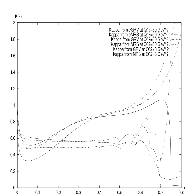
Figure 4: $\kappa(x)$ in terms of $x$ with two structure function sets and the evolved structure functions with two different sets. The solid, long dashed, short dashed, dotted, long dot-dashed, and short dot-dashed curves correspond to $\kappa(x)$ from the evolved structure functions with the GRV set and $Q^{2}=50$GeV², the evolved structure functions with the MRS set and $Q^{2}=50$GeV², the relevant structure functions of the GRV set with $Q^{2}=50$GeV², the relevant structure functions of the MRS set with $Q^{2}=50$GeV², the relevant structure functions of the GRV set with $Q^{2}=3$GeV², and the relevant structure functions of the MRS set with $Q^{2}=3$GeV².

We found interesting behavior in $\kappa(x)$. $\kappa(x)$ stays almost constant in $x$ after the use of the MRS set while it changes somewhat (it shoots up fast at low $x$) after the use of the GRV set as shown in the figure 4. The value of $\kappa$ also shows the interesting feature. Values of $\kappa$ both from GRV and MRS sets stay around 0.4 as shown in the table (*) and increase slowly for the smaller integration range of $x$ (i.e., bigger value of $x_{max}$ in the table). The value of $x_{max}$ should be ‘1’. Remember the definition of $\kappa$ in eq. (14). We chosed the lower limit of $x$ in the integration to be ‘0.001’. On the other hand, $\kappa$’s from our calculation stay around ‘0.6’. This is a big difference. The experimentally measured number of $\kappa$ may bring the way to improve our analysis further.

Table 1. First column, $x_{max}$, stands for the maximum value of the integration. For example, 0.1 value of $x$ corresponds to the integration range of $x$ of (0.001, 0.1) and 0.5 to the range of (0.001, 0.5). Second, third, fourth, and fifth columns in the table stand for the values of $\kappa$ using the structure functions directly from the GRV set, evolved results with the GRV functions, the structure functions directly from the MRS set, and evolved results with the MRS functions, respectively. In all cases, $Q^{2}=50$GeV².

Table 1. First column, $x_{max}$, stands for the maximum value of the integration. For example, 0.1 value of $x$ corresponds to the integration range of $x$ of (0.001, 0.1) and 0.5 to the range of (0.001, 0.5). Second, third, fourth, and fifth columns in the table stand for the values of $\kappa$ using the structure functions directly from the GRV set, evolved results with the GRV functions, the structure functions directly from the MRS set, and evolved results with the MRS functions, respectively. In all cases, $Q^{2}=50$GeV².

$x_{max}$ GRV eGRV MRS eMRS 0.1 0.382 0.618 0.477 0.636 0.2 0.390 0.614 0.479 0.629 0.3 0.402 0.616 0.480 0.625 0.4 0.411 0.619 0.481 0.622 0.5 0.419 0.621 0.481 0.621 0.6 0.424 0.623 0.481 0.620 0.7 0.428 0.624 0.481 0.620 0.8 0.430 0.625 0.482 0.619 0.9 0.432 0.626 0.482 0.619

Acknowledgments

This work was supported in part by the School Research Fund at Halla Institute of Technology. I would like to thank to YVRC at Yonsei University for the hospitality.

References

References

- [1] E. A. Kuraev, L. N. Liapatov, and V. S. Fadin, Sov. Phys. JETP 45 (1978) 199; Ya. Ya. Balistsky and L. N. Lipatov, Sov. J. Nucl. Phys. 28 (1978) 22.
- [2] C. Foudas et al. (CCFR), Phys. Rev. Lett. 64, (1990) 1207; S. A. Rabinowitz et al. (CCFR), Phys. Rev. Lett. 70 (1993) 134; James Botts et al. (CTEQ), Phys. Lett. B304, (1993) 159; H. L. Lai et al. (CTEQ), Phys. Rev. D55 (1997) 1280.
- [3] G. T. Garvey et al., Prog. Part. Nucl. Phys. 44 (2000) 305 and references therein.
- [4] For charged weak-current processes, refer V. Barone et al., Phys. Lett B317 (1993) 433; Phys. Lett. B328 (1994) 143; Z. Phys. C70 (1996) 83; V. Barone, U. D’Alesio, and M. Genovese, Phys. Lett. B357 (1995) 435; V. Barone and M. Genovese, Phys. Lett B379 233.
- [5] M. Glück, E. Hoffman, and E. Reya, Z. Phys. C13 (1982) 119.
- [6] V. N. Gribov and L. N. Lipatov, Sov. J. Nucl. Phys. 15 (1972) 78; V. N. Gribov and L. N. Lipatov, Sov. J. Nucl. Phys. 15 (1972) 438; Yu. L. Dokshitzer, Sov. Phys. JETP 73 (1977) 1216; Yu. L. Dokshitzer, Sov. Phys. JETP 46 (1977) 641; G. Altarelli and G. Parisi, Nucl. Phys. B126, (1977) 298.
- [7] C. S. Kim, S. M. Kim, and M. G. Olsson, MAD/PH/746, hep-ph/9307299 (unpublished).
- [8] M. Glück, E. Reya, and A. Vogt, Z. Phys. C53 (1992) 127.
- [9] A. D. Martin, R. G. Roberts, and W. J. Stirling, Phys. Rev. D47 (1993) 867.