Northwestern University:
N.U.H.E.P. Report No. 901
University of Wisconsin:
MADPH-01-1251
revised: November 26, 2001
On factorization, quark counting and vector dominance

Using an eikonal structure for the scattering amplitude, Block and Kaidalov[1] have derived factorization theorems for nucleon-nucleon, $\gamma p$ and $\gamma\gamma$ scattering at high energies, using only some very general assumptions. We present here an analysis giving experimental confirmation for factorization of cross sections, nuclear slope parameters B and $\rho$-values (ratio of real to imaginary portion of forward scattering amplitudes), showing that:

• the three factorization theorems[1] hold,

• the additive quark model holds to $\approx 1\%$,

• and vector dominance holds to better than $\approx 4\%$.

1 Introduction

Assuming factorizable eikonals in impact parameter space $b$ for nucleon-nucleon, $\gamma$p and $\gamma\gamma$ scattering processes whose opacities are equal, Block and Kaidalov[1] have proved three factorization theorems:

1. $$\frac{\sigma_{\rm nn}(s)}{\sigma_{\gamma\rm p}(s)}=\frac{\sigma_{\gamma\rm p}(s)}{\sigma_{\gamma\gamma}(s)},$$

   where the $\sigma$’s are the total cross sections for nucleon-nucleon, $\gamma$p and $\gamma\gamma$ scattering,

2. $$\frac{B_{\rm nn}(s)}{B_{\gamma\rm p}(s)}=\frac{B_{\gamma\rm p}(s)}{B_{\gamma\gamma}(s)},$$

   where the $B$’s are the nuclear slope parameters for elastic scattering,

3. $$\frac{\rho_{\rm nn}(s)}{\rho_{\gamma\rm p}(s)}=\frac{\rho_{\gamma\rm p}(s)}{\rho_{\gamma\gamma}(s)},$$

   where the $\rho$’s are the ratio of the real to imaginary portions of the forward scattering amplitudes,

with each factorization theorem having its own proportionality constant. These theorems are exact, for all $s$ (where $\sqrt{s}$ is the c.m.s. energy), and survive exponentiation of the eikonal[1].

Physically, the assumption of equal opacities, where the opacity is defined as the value of the eikonal at $b=0$, is the same as demanding that the ratios of elastic to total cross sections are equal, i.e.,

$$\left(\frac{\sigma_{\rm el}}{\sigma_{\rm tot}}\right)_{\rm nn}=\left(\frac{\sigma_{\rm el}}{\sigma_{\rm tot}}\right)_{\gamma\rm p}=\left(\frac{\sigma_{\rm el}}{\sigma_{\rm tot}}\right)_{\gamma\gamma},$$ (1)

as the energy goes to infinity[1].

Factorization theorem 1, involving ratios of cross sections, is perhaps the best known. Factorization theorems 2 and 3 are less known, but turn out to be of primary importance. The purpose of this note is to present strong experimental evidence for all three factorization theorems, as well as evidence for the additive quark model and vector dominance.

2 Eikonal Model

In an eikonal model[3], a (complex) eikonal $\chi(b,s)$ is defined such that $a(b,s)$, the (complex) scattering amplitude in impact parameter space $b$, is given by

$$a(b,s)=\frac{i}{2}\left(1-e^{i\chi(b,s)}\right)=\frac{i}{2}\left(1-e^{-\chi_{{}_{\rm I}}(b,s)+i\chi_{{}_{\rm R}}(b,s)}\right).$$ (2)

Using the optical theorem, the total cross section $\sigma_{\rm tot}(s)$ is given by

$$\sigma_{\rm tot}(s)=2\int\,\left[1-e^{-\chi_{{}_{\rm I}}(b,s)}\cos(\chi_{{}_{\rm R}}(b,s))\right]\,d^{2}\vec{b},$$ (3)

the elastic scattering cross section $\sigma_{\rm el}(s)$ is given by

$$\sigma_{\rm elastic}(s) = \int\left|1-e^{-\chi_{{}_{\rm I}}(b,s)+i\chi_{{}_{\rm R}}(b,s)}\right|^{2}\,d^{2}\vec{b}$$ (4)

and the inelastic cross section, $\sigma_{\rm inelastic}(s)$, is given by

$$\sigma_{\rm inelastic}(s)=\sigma_{\rm tot}(s)-\sigma_{\rm elastic}(s)=\int\,\left[1-e^{-2\chi_{{}_{\rm I}}(b,s)}\right]\,d^{2}\vec{b}.$$ (5)

The ratio of the real to the imaginary part of the forward nuclear scattering amplitude, $\rho$, is given by

$$\rho(s) = \frac{{\rm Re}\left\{i(\int 1-e^{-\chi_{{}_{\rm I}}(b,s)+i\chi_{{}_{\rm R}}(b,s)})\,d^{2}\vec{b}\right\}}{{\rm Im}\left\{i(\int(1-e^{-\chi_{{}_{\rm I}}(b,s)+i\chi_{{}_{\rm R}}(b,s)})\,d^{2}\vec{b}\right\}}$$ (6)

and the nuclear slope parameter $B$ is given by

$$B=\frac{\int\,b^{2}a(b,s)\,d^{2}\vec{b}}{2\int\,a(b,s)\,d^{2}\vec{b}}.$$ (7)

2.1 Even Eikonal

A description of the forward proton–proton and proton–antiproton scattering amplitudes is required which is analytic, unitary, satisfies crossing symmetry and the Froissart bound. A convenient parameterization[2, 3] consistent with the above constraints and with the high-energy data can be constructed in a model where the asymptotic nucleon becomes a black disk as a reflection of particle (jet) production. The increase of the total cross section is the shadow of jet-production which is parameterized in parton language. The picture does not reproduce the lower energy data which is simply parameterized using Regge phenomenology. The even QCD-inspired eikonal $\chi_{\rm even}$ for nucleon-nucleon scattering[2, 3] is given by the sum of three contributions, gluon-gluon, quark-gluon and quark-quark, which are individually factorizable into a product of a cross section $\sigma(s)$ times an impact parameter space distribution function $W(b\,;\mu)$, i.e.,:

$$\chi^{\rm even}(s,b) = \chi_{\rm gg}(s,b)+\chi_{\rm qg}(s,b)+\chi_{\rm qq}(s,b)$$ (8)

$$= i\left[\sigma_{\rm gg}(s)W(b\,;\mu_{\rm gg})+\sigma_{\rm qg}(s)W(b\,;\sqrt{\mu_{\rm qq}\mu_{\rm gg}})+\sigma_{\rm qq}(s)W(b\,;\mu_{\rm qq})\right],$$

where the impact parameter space distribution function is the convolution of a pair of dipole form factors:

$$W(b\,;\mu)=\frac{\mu^{2}}{96\pi}(\mu b)^{3}K_{3}(\mu b).$$ (9)

It is normalized so that $\int W(b\,;\mu)d^{2}\vec{b}=1.$ Hence, the $\sigma$’s in eq. (8) have the dimensions of a cross section. The factor $i$ is inserted in eq. (8) since the high energy eikonal is largely imaginary (the $\rho$ value for nucleon-nucleon scattering is rather small).

The opacity of the eikonal, its value at $b=0$, is given by

$${\rm O}^{\rm nn}=\frac{i}{12\pi}\left[\sigma_{\rm gg}(s)\mu_{\rm gg}^{2}+\sigma_{\rm qg}(s)\mu_{\rm qg}^{2}+\sigma_{\rm qq}(s)\mu_{\rm qq}^{2}\right],$$ (10)

a simple sum of the products of the appropriate cross sections $\sigma$ with the $\mu^{2}$’s, a result which we will utilize later.

2.2 Odd Eikonal

The odd eikonal, $\chi_{odd}(b,s)=i\sigma_{odd}\,W(b;\mu_{odd})$, accounts for the difference between $pp$ and $p\bar{p}$, and must vanish at high energies. A Regge behaved analytic odd eikonal can be parametrized as (see Eq. (5.5b) of Ref. [4])

$$\chi_{odd}(b,s)=-\,C_{odd}\Sigma_{gg}\frac{m_{0}}{\sqrt{s}}\,e^{i\pi/4}\,W(b;\mu_{odd})\,$$ (11)

where $\mu_{\rm odd}$ is determined by experiment and the normalization constant $C_{odd}$ is to be fitted.

2.3 Total Eikonal

The data for both $pp$ and $\bar{p}p$ are fitted using the total eikonal

$$\chi^{\bar{p}p}_{pp}=\chi_{\rm even}\pm\chi_{\rm odd}.$$ (12)

3 A Global Fit of Accelerator and Cosmic Ray Data

Using an eikonal analysis in impact parameter space, Block et al. [2, 3, 6] have constructed a QCD-inspired parameterization of the forward proton–proton and proton–antiproton scattering amplitudes which fits all accelerator data[5] for $\sigma_{\rm tot}$, nuclear slope parameter $B$ and $\rho$, the ratio of the real-to-imaginary part of the forward scattering amplitude for both $pp$ and $\bar{p}p$ collisions, using a $\chi^{2}$ procedure and the eikonal of eq. (12); see Fig. 1 and Fig. 2

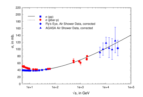
Figure 1: The fitted $\sigma_{pp}$ and $\sigma_{\bar{p}p}$, in mb vs. $\sqrt{s}$, in GeV, for the QCD-inspired fit of total cross section, $B$ and $\rho$ for both $pp$ and $\bar{p}p$. The accelerator data (squares are pp and circles are $\bar{\rm p}$p ) and the cosmic ray points (diamond, Fly’s Eye and triangles, AGASA) have been fitted simultaneously. The cosmic ray data that are shown have been converted from $\sigma_{p{-}\rm air}^{\rm inel}$ to $\sigma_{pp}$.

which are taken from ref. [6]—in addition, the high energy cosmic ray cross sections of Fly’s Eye [7] and AGASA [8] experiments are also simultaneously fit[6]. Because the parameterization is both unitary and analytic, its high energy predictions are effectively model–independent, if you require that the proton is asymptotically a black disk. A major difference between simultaneously fitting the cosmic ray and accelerator data and earlier results in which only accelerator data were used, is a lowering (by about a factor of $\approx 2$) of the error of the predictions for the high energy cross sections. In particular, the error in $\sigma_{pp}$ at $\sqrt{s}=30$ TeV is reduced to $\approx 1.5$ %, because of significant reductions in the errors estimated for the fit parameters (for a more complete explanation, see ref. [6]).

The plot of $\sigma_{pp}$ vs. $\sqrt{s}$, including the cosmic ray data, is shown in Fig. 1, which was taken from ref. [6]. The overall agreement between the accelerator and the cosmic ray $pp$ cross sections with the QCD-inspired fit, as shown in Fig. 1, is striking.

In brief, the eikonal description provides an excellent description of the experimental data at high energy for both $pp$ and $\bar{p}p$ scattering at high energies.

4 Factorization

We emphasize that the QCD-inspired parameterization of the $pp$ and $\bar{p}p$ data [2, 3, 6] allows us to calculate accurately the even eikonal of eq. (8) needed for:

• the total cross section $\sigma_{\rm nn}$ (from eq. (3)) used in the factorization theorem 1,

• the nuclear slope parameter $B_{\rm nn}$ (from eq. (7)) used in the factorization theorem 2,

• and the $\rho$-value $\rho_{\rm nn}$ (from eq. (6)) used in the factorization theorem 3,

since we must compare nn to $\gamma p$ and $\gamma\gamma$ reactions.

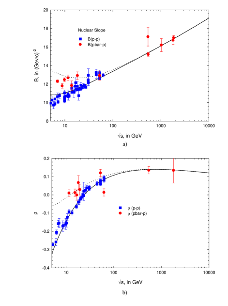
Figure 2: The fitted values for the nuclear slope parameters $B_{pp}$ and $B_{\bar{p}p}$, in (GeV/c)^-2 vs. $\sqrt{s}$, in GeV, for the QCD-inspired fit are shown in (a). In (b), the fitted values for $\rho_{\bar{p}p}$ and $\rho_{pp}$ are shown.

4.1 Theorems

As shown in ref. [1], the eikonals for $\gamma p$ and $\gamma\gamma$ scattering that satisfy eq. (1)are given by

$$\chi^{\gamma p}(s,b)=i\left[\kappa\sigma_{\rm gg}(s)W(b\,;\sqrt{\frac{1}{\kappa}}\mu_{\rm gg})+\kappa\sigma_{\rm qg}(s)W(b\,;\sqrt{\frac{1}{\kappa}}\sqrt{\mu_{\rm qq}\mu_{\rm gg}}+\kappa\sigma_{\rm qq}(s)W(b\,;\sqrt{\frac{1}{\kappa}}\mu_{\rm qq})\right],$$ (13)

and

$$\chi^{\gamma\gamma}(s,b)=i\left[\kappa^{2}\sigma_{\rm gg}(s)W(b\,;\frac{1}{\kappa}\mu_{\rm gg})+\kappa^{2}\sigma_{\rm qg}(s)W(b\,;\frac{1}{\kappa}\sqrt{\mu_{\rm qq}\mu_{\rm gg}}+\kappa^{2}\sigma_{\rm qq}(s)W(b\,;\frac{1}{\kappa}\mu_{\rm qq})\right],$$ (14)

where we obtain $\chi^{\gamma p}$ from $\chi^{\rm even}$ from multiplying each $\sigma$ in $\chi^{\rm even}$ by $\kappa$ and each $\mu$ by $\sqrt{\frac{1}{\kappa}}$, and, in turn, we next obtain $\chi^{\gamma\gamma}$ from $\chi^{\gamma p}$ from multiplying each $\sigma$ in $\chi^{\gamma p}$ by $\kappa$ and each $\mu$ by $\sqrt{\frac{1}{\kappa}}$. The $\kappa$ in eq. (13) and eq. (14) is an energy-independent proportionality constant. We emphasize that the same $\kappa$ must be used in the gluon sector as in the quark sector for the ratio of $\left(\frac{\sigma_{\rm el}}{\sigma_{\rm tot}}\right)$ to be process-independent (see eq. (1). The functional forms of the impact parameter distributions are assumed to be the same for $\gamma p$, $\gamma\gamma$ and $nn$ reactions. It is clear from using eq. (9), eq. (13), eq. (14) and then comparing to the opacity of eq. (10), that the three opacities are all the same, i.e.,

$$O^{\rm nn}=O^{\gamma p}=O^{\gamma\gamma}=\frac{i}{12\pi}\left[\sigma_{\rm gg}(s)\mu_{\rm gg}^{2}+\sigma_{\rm qg}(s)\mu_{\rm qg}^{2}+\sigma_{\rm qq}(s)\mu_{\rm qq}^{2}\right].$$ (15)

Hence, from ref. [1], we have the three factorization theorems

$$\frac{\sigma_{\rm nn}(s)}{\sigma_{\gamma\rm p}(s)} = \frac{\sigma_{\gamma\rm p}(s)}{\sigma_{\gamma\gamma}(s)}$$ (16)

$$\frac{B_{\rm nn}(s)}{B_{\gamma\rm p}(s)} = \frac{B_{\gamma\rm p}(s)}{B_{\gamma\gamma}(s)}$$ (17)

$$\frac{\rho_{\rm nn}(s)}{\rho_{\gamma\rm p}(s)} = \frac{\rho_{\gamma\rm p}(s)}{\rho_{\gamma\gamma}(s)},$$ (18)

valid for all $s$. It is easily inferred from ref. [1] that

$$\sigma_{\gamma\gamma}(s) =\kappa P_{\rm had}^{\gamma}\sigma_{\gamma\rm p}(s) ={\left(\kappa P_{\rm had}^{\gamma}\right)}^{2}\sigma_{\rm nn}(s)$$ (19)

$$B_{\gamma\gamma}(s) =\kappa B_{\gamma\rm p}(s) =\kappa^{2}B_{\rm nn}(s)$$ (20)

$$\rho_{\gamma\gamma}(s) =\rho_{\gamma\rm p}(s) =\rho_{\rm nn}(s),$$ (21)

where $P_{\rm had}^{\gamma}$ is the probability that a photon transforms into a hadron, assumed to be independent of energy and $\kappa$ is a proportionality constant, also independent of energy. The value of $\kappa$, of course, is model-dependent. For the case of the additive quark model, $\kappa=\frac{2}{3}$.

We emphasize the importance of the result of eq. (21) that the $\rho$’s are all equal, independent of the assumed value of $\kappa$, i.e., the equality does not depend on the assumed model.

4.2 Experimental Verification of Factorization using Compton Scattering

The solid curve in Fig. 3

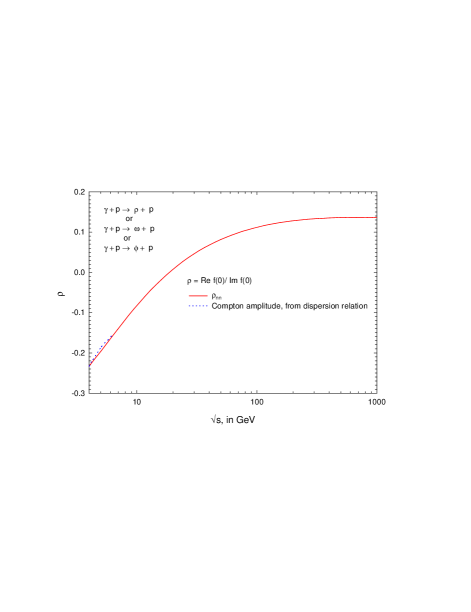
Figure 3: The solid curve is $\rho_{\rm nn}$, the predicted ratio of the real to imaginary part of the forward scattering amplitude for the ‘elastic’ reactions , $\gamma+p\rightarrow V+p$ scattering amplitude, where $V$ is $\rho$, $\omega$ or $\phi$ (using the factorization theorem of eq. (21)). The dotted curve is ratio of the real to imaginary part of the forward scattering amplitude for Compton scattering , $\gamma+p\rightarrow\gamma+p$, found from dispersion relations[9]. It has been slightly displaced from the solid curve for clarity in viewing.

is $\rho_{\rm nn}$, plotted as a function of the c.m.s. energy $\sqrt{s}$. According to eq. (21), this should be the same as $\rho_{\gamma\rm p}$. No experimental data for the ‘elastic scattering’ reactions $\gamma+p\rightarrow V+p$, where $V$ is the vector meson $\rho$, $\omega$ or $\phi$, are available for direct comparison. However, Damashek and Gilman [9] have calculated the $\rho$ value for Compton scattering $\gamma+p\rightarrow\gamma+p$ using dispersion relations, i.e., the true elastic scattering reaction for photon-proton scattering. The dispersion relation calculation gives $\rho_{\gamma\rm p}$ if we assume that it is the same as that for the ‘elastic scattering’ reactions $\gamma+p\rightarrow V+p$. In this picture we expect that $B_{\gamma\rm p}=B_{\rho}=B_{\omega}=B_{\phi}$. We then compare the dispersion relation calculation, the dotted line in Fig. 3, with our prediction for $\rho_{\gamma\rm p}$ from eq. (21) ($\rho_{\rm nn}$, the solid line taken from ref. [6]). The agreement is so close that the two curves had to be moved apart so that they may be viewed more clearly. It is clearly of importance to extend the energy region of the dispersion calculation. However, over the limited energy range available from the dispersion calculation, the prediction from eq. (21) of equal $\rho$-values is well verified experimentally.

4.3 Quark Counting

The additive quark model tells us from quark counting that $\kappa$ in eq. (20) is given by $\kappa=\frac{2}{3}$. We can experimentally determine $\kappa$ by invoking from eq. (20) the relation $B_{\gamma\rm p}=\kappa B_{\rm nn}$ ($B_{\rm nn}$ is computed using the parameters from ref. [6]), and fitting $\kappa$. In our picture, the ‘elastic scattering’ reactions $\gamma+p\rightarrow V+p$, where $V$ is the vector meson $\rho$, $\omega$ or $\phi$, require that $B_{\rho}=B_{\omega}=B_{\phi}(=B_{\gamma\rm p})$. To determine the value of $\kappa$ in the relation $B_{\gamma\rm p}=\kappa\,B_{\rm nn}$, a $\chi^{2}$ fit was made to the available $B_{\gamma\rm p}$ data. In Fig. 4 we plot $\kappa B_{\rm nn}$ vs. the c.m.s. energy $\sqrt{s}$, using the best-fit value of $\kappa=0.661$, against the experimental values of $B_{\gamma\rm p}$. The fit gave $\kappa=0.661\pm 0.008$, with a total $\chi^{2}=16.4$ for 10 degrees of freedom. Inspection of Fig. 4 shows that the experimental point of $B_{\rho}$ at $\sqrt{s}=5.2$ GeV— which contributes 6.44 to the $\chi^{2}$—clearly cannot lie on any smooth curve and thus can safely be ignored. Neglecting the contribution of this point gives a $\chi^{2}$/d.f.=0.999, a very satisfactory result. We emphasize that the experimental $\gamma p$ data thus

• require $\kappa=0.661\pm 0.008$, a $\approx 1\%$ measurement in excellent agreement with the value of 2/3 that is obtained from the additive quark model.

• clearly verify the nuclear slope factorization theorem of eq. (20) over the available energy range spanned by the data.

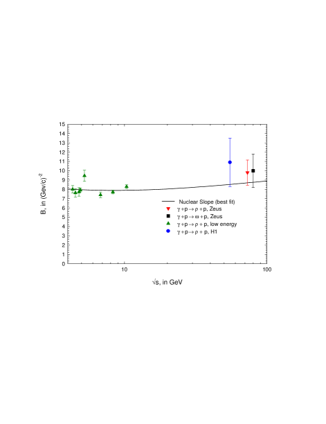
Figure 4: A $\chi^{2}$ fit of experimental data for the nuclear slopes $B$, from the ‘elastic scattering’ reactions $\gamma+p\rightarrow V+p$, where $V$ is $\rho$, $\omega$ or $\phi$, to the relation $B_{\gamma\rm p}=\kappa B_{\rm nn}$, of eq. (20), where $\kappa=0.661\pm 0.008$

For additional evidence involving the equality of the nuclear slopes $B_{\rho}$, $B_{\gamma}$ and $B_{\phi}$ from differential elastic scatttering data $\frac{d\sigma}{dt}$, see Figures (13,14,15) of ref. [3].

4.4 Vector Dominance, using $\gamma p$ Cross Sections

Using $\kappa=\frac{2}{3}$ and eq. (19), we write

$$\sigma_{\gamma\rm p}(s)=\frac{2}{3}P_{\rm had}^{\gamma}\,\sigma_{\rm nn}(s),$$ (22)

where $P_{\rm had}^{\gamma}$ is the probability that a photon will interact as a hadron. We will use the value $P_{\rm had}^{\gamma}=1/240$. This value is approximately 4% greater than that derived from vector dominance, 1/249. Using (see Table XXXV, pag. 393 of ref. [10]) $f_{\rho}^{2}/4\pi=2.2$, $f_{\omega}^{2}/4\pi=23.6$ and $f_{\phi}^{2}/4\pi=18.4$, we find $\Sigma_{V}(4\pi\alpha/f_{V}^{2})=1/249$, where $V=\rho,\omega,\phi$. The value we use of 1/240 is found by normalizing the total $\gamma p$ cross section to the low energy data and is illustrated in Fig. 5, where we plot the total cross section for $\gamma+p\rightarrow{\rm hadrons}$ from eq. (22) as a function of the c.m.s. energy $\sqrt{s}$. The values for $\sigma_{\rm nn}$ have been deduced from the results of ref. [6], using the even eikonal from eq. (8). The fit is exceptionally good, reproducing the rising cross section for $\gamma p$, using the parameters fixed by nucleon-nucleon scattering. The fact that we use the value 1/240 rather than 1/249 (4% greater than the vector meson prediction) reflects the fact that $P_{\rm had}^{\gamma}$, the total probability that the photon is a hadron, should have a small contribution from the continuum, as well as from the vector mesons $\rho$, $\phi$ and $\omega$. Thus, within the uncertainties of our calculation, the experimental data in the $\gamma p$ sector

• are compatible with vector meson dominance.

• agree with cross section factorization theorem of eq. (19).

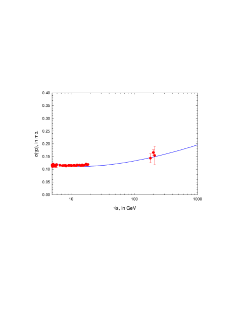
Figure 5: The total cross section for $\gamma p$ scattering. The solid curve is the predicted total cross section from the factorization relation of eq. (19), $\sigma_{\gamma\rm p}=\frac{2}{3}P_{\rm had}^{\gamma}\,\sigma_{\rm nn}$, where $P_{\rm had}^{\gamma}=1/240$.

4.5 Experimental Verification of Factorization using $\gamma\gamma$ Scattering

Using quark counting and the factorization theorem of eq. (19), we now write $\sigma_{\gamma\gamma}={\left(\frac{2}{3}P_{\rm had}^{\gamma}\right)}^{2}\,\sigma_{\rm nn}$ where $P_{\rm had}^{\gamma}=1/240$. In Fig. 6

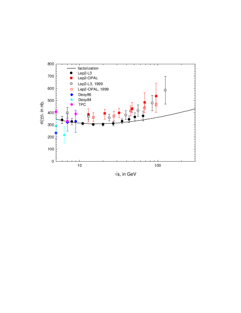
Figure 6: The predicted total cross section for $\gamma\gamma$ scattering from the factorization theorem of eq. (19), $\sigma_{\gamma\gamma}={\left(\frac{2}{3}P_{\rm had}^{\gamma}\right)}^{2}\,\sigma_{\rm nn}$, where $P_{\rm had}^{\gamma}=1/240$. The data sources are indicated in the legend.

we plot our factorization prediction for $\sigma_{\gamma\gamma}(s)$ as a function of the c.m.s. energy $\sqrt{s}$ and compare it to various sets of experimental data. It is clear that factorization, as expressed in eq. (19), selects the preliminary L3 data (solid circles) rather than the preliminary OPAL results (solid squares) [11]. The Monte Carlo-averaged final results of L3, given by the open circles, agrees, within errors, with the revised OPAL data, with both new sets having a normalization of about 15-20 % higher than the factorization prediction given by the solid line. The major difference between the earlier L3 result and the revised data was the use of the average normalization from the output of two different Monte Carlos. We find it remarkable that the cross section factorization theorem of eq. (19), using only input from the additive quark model and vector meson dominance, gives a reasonable prediction of the experimental data over a cross section magnitude span of more than a factor of $10^{5}$ and an energy region of $3\leq\sqrt{s}\leq 100$ GeV. On the other hand, a literal interpretation of the experimental data at the higher energies might indicate that the $\gamma\gamma$ cross section is rising slightly more rapidly than our prediction, a consequence perhaps of hard processes not accounted for by the vector dominance model. More accurate data are required for confirmation of this hypothesis.

5 Conclusions

The available data on nn, $\gamma p$ and $\gamma\gamma$ reactions lend strong experimental support to the factorization hypotheses of

• the well-known cross section factorization theorem of eq. (16) and eq. (19),

• the lessor-known nuclear slope factorization theorem of eq. (17) and eq. (20),

• the relatively obscure requirement of eq. (21) that $\rho_{\rm nn}=\rho_{\gamma\rm p}=\rho_{\gamma\gamma}$,

as well as

• verifying the additive quark model by measuring $\kappa=0.661\pm 0.008$, a result within $\approx 1\%$ of the value of 2/3 expected for the quark model, using $B_{\gamma\rm p}$ measurements over a wide span of energies, $3\leq\sqrt{s}\leq 200$.

• confirming vector dominance using $\sigma_{\rm nn}$, $\sigma_{\gamma\rm p}$ and $\sigma_{\gamma\gamma}$ over an energy region of $3\leq\sqrt{s}\leq 100$ GeV and a cross section factor of over $10^{5}$.

  The QCD-inspired model[3] that we use fits the $pp$ and $\bar{p}p$ data on total cross sections, $\rho$-values and $B$ quite well and thus gives a good phenomological fit to those data. We emphasize that the conclusions on factorization that we presented above are rooted in the available high energy experimental data for nn, $\gamma p$ and $\gamma\gamma$ collisions and do not depend on the details of the model used to fit nn data.

Appendix A Appendix

For completeness, we summarize here the formulae and parameters needed to calculate nucleon-nucleon scattering, taken from ref. [3] and ref. [6], which should be consulted for more detail.

We model the gluon-gluon contribution to the nucleon-nucleon cross section following the parton model

$$\sigma_{gg}(s)=C_{gg}\int\Sigma_{gg}\,\Theta(\hat{s}-m_{0}^{2})F_{gg}(x_{1},x_{2})\,d\tau\;,$$ (23)

where $\Sigma_{gg}=9\pi\alpha_{s}^{2}/m_{0}^{2}$ is a normalization constant, ${\hat{s}}=\tau s$, and

$$F_{gg}=\int\!\!\int f_{g}(x_{1})f_{g}(x_{2})\delta(\tau-x_{1}x_{2})\,dx_{1}\,dx_{2}\;.$$ (24)

Note that for the parameterization of the gluon structure function as $f_{g}(x)=N_{g}(1-x)^{5}/x^{1+\epsilon}$, where $N_{g}=\frac{1}{2}(6-\epsilon)(5-\epsilon)\cdots(1-\epsilon)/5!$, we can carry out explicitly the integrations, obtaining

$$\sigma_{\rm gg}(s)=C^{\prime}_{\rm gg}\Sigma_{\rm gg}N_{\rm g}^{2}\sum_{i=0}^{5}\left\{\frac{a(i)-\frac{b(i)}{i-\epsilon}}{i-\epsilon}-\tau_{0}^{i-\epsilon}\left(\frac{a(i)-\frac{b(i)}{i-\epsilon}}{i-\epsilon}+\frac{b(i)}{i-\epsilon}\log(\tau_{0})\right)\right\}$$ (25)

where $C^{\prime}_{\rm gg}=C_{\rm gg}/9$, $\tau_{0}=m_{0}^{2}/s$, $a(0)=-a(5)=-411/10$, $a(1)=-a(4)=-975/2,$ $a(2)=-a(3)=-600$, $b(0)=b(5)=-9,$ $b(1)=b(4)=-225,$ and $b(2)=b(3)=-900$. The normalization constant $C^{\prime}_{gg}$ is a fitted parameter and the threshold mass $m_{0}$ is determined by experiment. The role of $m_{0}$, which is the onset of $\sigma_{gg}(s)$ with $\hat{s}$, is somewhat analagous to the role played by $p_{T}^{min}$ in the minijet models. However, numerical exercises show that the value of $m_{0}$ is not dependent on energy and that the fit is not very sensitive to the value.

Also our quark-quark and quark-gluon cross sections will be parameterized following the scaling parton model. We approximate the quark-quark contribution with

$$\sigma_{qq}(s)=\Sigma_{gg}\left(C+C_{Regge}^{even}\frac{m_{0}}{\sqrt{s}}\right)\;,$$ (26)

where $C$ and $C_{Regge}^{even}$ are parameters to be fitted. The quark-gluon interaction is approximated as

$$\sigma_{qg}(s)=\Sigma_{gg}C_{qg}^{log}\log\frac{s}{s_{0}},$$ (27)

where the normalization constant $C_{qg}^{log}$ and the square of the energy scale in the log term $s_{0}$ are parameters are parameters to be fitted.

In summary, the even contribution to the eikonal is

$$\chi_{even} = i\left\{\sigma_{gg}(s)W(b\,;\mu_{gg})+\Sigma_{gg}\left(C+C_{Regge}^{even}\frac{m_{0}}{\sqrt{s}}\right)W(b\,;\mu_{qq})\right.$$ (28)

$$\left.+\Sigma_{gg}C_{qg}^{log}\log\frac{s}{s_{0}}W(b\,;\sqrt{\mu_{qq}\mu_{gg}})\right\}\;.$$

The total even contribution is not yet analytic. For large $s$, the even amplitude in eq. (8) is made analytic by the substitution (see the table on p. 580 of reference [4], along with reference [12]) $s\rightarrow se^{-i\pi/2}.$ The quark contribution $\chi_{\rm qq}(s,b)$ accounts for the constant cross section and a Regge descending component ($\propto 1/\sqrt{s}$), whereas the mixed quark-gluon term $\chi_{\rm qg}(s,b)$ simulates diffraction ($\propto\log s$). The gluon-gluon term $\chi_{\rm gg}(s,b)$, which eventually rises as a power law $s^{\epsilon}$, accounts for the rising cross section and dominates at the highest energies. In eq. (8), the inverse sizes (in impact parameter space) $\mu_{\rm qq}$ and $\mu_{\rm gg}$ are determined by experiment, whereas the quark-gluon inverse size is taken as $\sqrt{\mu_{\rm qq}\mu_{\rm gg}}$.

Fitted	Fixed
$C=5.65\pm 0.14$	$\alpha_{s}=0.5$
$C^{log}_{qg}=0.103\pm 0.026$	$\epsilon=0.05$
$C^{\prime}_{gg}=(1.12\pm 0.05)\times 10^{-3}$	$m_{0}=0.6$ GeV
$C^{even}_{Regge}=25.3\pm 2.0$	$\mu_{qq}=0.89$ GeV
$C_{odd}=7.62\pm 0.28$	$\mu_{gg}=0.73$ GeV
$s_{0}=16.9\pm 4.9$ GeV2	$\mu_{odd}=0.53$ GeV
	$k=1.349\pm 0.045$

Table 1: Value of the parameters.

In addition to the parameters in ref. [3], the cosmic ray data fit requires the specification of another parameter $k$, the proportionality constant between the measured mean free path (in air) and the true mean free path in air. The major difference between the parameters of Table 1 and the parameters of ref. [3] is that the errors of $C^{\prime}_{gg}$ and $s_{0}$ are now smaller by a factor of $\approx 2$, due to the large lever arm of the hign energy cosmic ray points. This in turn leads to significantly smaller errors in our predictions for high energy cross sections, since the dominant term at high energies is $\sigma_{\rm gg}(s)$.

References

• [1] M. M. Block and A. B. Kaidalov, “Consequences of the Factorization Hypothesis in $\bar{p}p,\ pp,\ \gamma p\ {\rm and\ }\gamma\gamma$ Collisions”, e-Print Archive: hep-ph/0012365, Northwestern University preprint N.U.H.E.P No. 712, Nov. 2000.
• [2] M. M. Block et al., Phys. Rev. D45, 839 (1992).
• [3] M. M. Block et al., e-Print Archive: hep-ph/9809403, Phys. Rev. D60, 054024 (1999).
• [4] M. M. Block and R. N. Cahn, Rev. Mod. Phys. 57, 563 (1985).
• [5] The accelerator data the of the new E-811 high energy cross section at the Tevatron has been included: C. Avila et al., Phys. Lett. B 445, 419 (1999).
• [6] M. M. Block et al., e-Print Archive: hep-ph/0004232, Phys. Rev. D62, 077501 (2000).
• [7] R. M. Baltrusaitis et al., Phys. Rev. Lett. 52, 1380 (1984).
• [8] M. Honda et al., Phys. Rev. Lett. 70, 525 (1993).
• [9] M. Damashek and F.J. Gilman, Phys. Rev. D1,1319 (1970).
• [10] T.H. Bauer et al., Rev. Mod. Phys. 50, 261 (1978).
• [11] PLUTO Collaboration, Ch. Berger et al., Phys. Lett. B149, 421 (1984); TPC/2$\gamma$ Collaboration, H. Aihara et al., Phys. Rev. D41, 2667 (1990); MD-1 Collaboration, S.E. Baru et al., Z. Phys. C53, 219 (1992); L3 Collaboration, M. Acciarri et al., Phys. Lett. B408, 450 (1997); F. Wäckerle, “Total Hadronic Cross-Section for Photon-Photon Interactions at LEP”, to be published in the Proceedings of the XXVII International Symposium on Multiparticle Dynamics, Frascati, September 1997, and Nucl. Phys.  B, Proc. Suppl.
• [12] Eden, R. J., “High Energy Collisions of Elementary Particles”, Cambridge University Press, Cambridge (1967).