On the structure of the pion:
A QCD–inspired point of view

Abstract

The effective interaction between a quark and an anti-quark as obtained previously with by the method of iterated resolvents is replaced by the so called up-down-model and applied to flavor off-diagonal mesons including the pion. The only free parameters are those of canonical quantum chromo-dynamics (QCD), particularly the coupling constant and the masses of the quarks.

The so obtained light-cone wave function can be used to calculate the pion’s form factor, particularly its mean-square radius can be computed analytically. The results allow for the exciting conclusion that the pion is built by highly relativistic constituents, in strong contrast to composite systems like atoms or nuclei with non-relativistic constituents.

1 Introduction

One of the most urgent problems in contemporary physics is to compute the structure of hadrons in terms of their constituents, based on a covariant theory such as QCD.

Among the hadrons the pion is the most mysterious particle. I have proposed an oversimplified model, the $\uparrow\downarrow$-model, which has many drawbacks but the virtue of being inspired by QCD and of having the same number of parameters one expects in a full theory: namely the 6 flavor quark masses, the strong coupling constant (7) and one additional scale parameter (8) originating in the murky depth of renormalization theory.

The model is QCD-inspired by virtue of the fact, that it is based on the full light-cone Hamiltonian as obtained from the QCD-Lagrangian in the light-cone gauge, with zero-modes disregarded. In consequence, the pion is treated on the same footing as all other pseudo-scalar and pseudo-vector mesons.

The model should be contrasted to Lattice Gauge Calculations, see for example [1]. It is not generally known that LGC’s have considerable uncertainty to extrapolate their results down to such light mesons as a pion. It is also not generally known that lattice gauge calculations get always strict and linear confinement even for QED, where we know the ionization threshold. The ‘breaking of the string’, or in a more physical language, the ionization threshold is one of the hot topics at the lattice conferences [2]. Moreover, in order to get the size of the pion, thus the form factor, another generation of computers is required, as well as physicists to run them.

The model should be contrasted also to phenomenological approaches. They usually do not address to get the pion. For the heavy mesons, where they are so successful [3], phenomenological model have quite many parameters, in any case more that the above canonical ones. A detailed comparison and systematic discussion of the bulky literature can however be postponed, until we are ready to solve the full Eq.(11).

The model should be contrasted, finally, to Nambu-Jona-Lasinio-like models which are so successful in accounting for isospin-aspects. I cannot quote the huge body of literature but mention in passing that the NJL-models are not renormalizable, that NJL has no relation to QCD, and that NJL deals mostly with the very light mesons. There is no way to treat the heavy flavors, see also [4].

2 Motivation

The light-cone approach to the bound-state problem in gauge theory [5] aims at solving $H_{LC}|\Psi\rangle=M^{2}|\Psi\rangle$. If one disregards possible zero modes and works in the light-cone gauge, the (light-cone) Hamiltonian $H_{LC}$ is a well defined Fock-space operator and given in [5]. Its eigenvalues are the invariant mass-squares $M^{2}$ of physical particles associated with the eigenstates $|\Psi\rangle$. In general, they are superpositions of all possible Fock states with its many-particle configurations. For a meson, for example, holds

$\displaystyle\begin{array}[]{rclllllll}{|\Psi_{\rm meson}\rangle}&=&{\sum\limits_{i}\ }{\Psi_{q\bar{q}}(x_{i},\vec{k}_{\!\perp_{i}},\lambda_{i})}{|q\bar{q}\rangle}&+&{\sum\limits_{i}\ }{\Psi_{gg}(x_{i},\vec{k}_{\!\perp_{i}},\lambda_{i})}{|gg\rangle}\\ &+&{\sum\limits_{i}\ }{\Psi_{q\bar{q}g}(x_{i},\vec{k}_{\!\perp_{i}},\lambda_{i})}{|q\bar{q}g\rangle}&+&{\sum\limits_{i}\ }{\Psi_{q\bar{q}q\bar{q}}(x_{i},\vec{k}_{\!\perp_{i}},\lambda_{i})}{|q\bar{q}q\bar{q}\rangle}&+&{\dots}\ .\end{array}$

If all wave functions like $\Psi_{q\bar{q}}$ or $\Psi_{gg}$ are available, one can analyze hadronic structure in terms of quarks and gluons [5].

For example, one can calculate the space-like form factor of a hadron quite straightforwardly. As illustrated in Fig. 2, it is just a sum of overlap integrals analogous to the corresponding non-relativistic formula [5]:

$$F(q^{2})=\sum_{n,\lambda_{i}}\sum_{a}e_{a}\int\overline{\prod_{i}}\ {dx_{i}\,d^{2}\vec{k}_{\perp}{}_{i}\over 16\pi^{3}}\,\psi_{n}^{(\Lambda)*}(x_{i},\vec{\ell}_{\perp}{}_{i},\lambda_{i})\,\psi_{n}^{(\Lambda)}(x_{i},\vec{k}_{\perp}{}_{i},\lambda_{i}).$$ (1)

Here $e_{a}$ is the charge of the struck quark, $\Lambda^{2}\gg\vec{q}_{\perp}^{\,2}$, and

$$\vec{\ell}_{\perp}{}_{i}\equiv\cases{\vec{k}_{\perp}{}_{i}-x_{i}\vec{q}_{\perp}+\vec{q}_{\perp}&\hbox{for the struck quark}\cr\vec{k}_{\perp}{}_{i}-x_{i}\vec{q}_{\perp}&\hbox{for all other partons,}\cr}$$

with $\vec{q}_{\perp}^{\,2}=Q^{2}=-q^{2}$. All of the various form factors of hadrons with spin can be obtained by computing the matrix element of the plus current between states of different initial and final hadron helicities.

3 The method of iterated resolvents

Because of the inherent divergencies in a gauge field theory, the QCD-Hamiltonian in 3+1 dimensions must be regulated from the outset. One of the few practical ways is vertex regularization [5, 6], where every Hamiltonian matrix element, particularly those of the vertex interaction (the Dirac interaction proper), is multiplied with a convergence-enforcing momentum-dependent function. It can be viewed as a form factor [5]. The precise form of this function is unimportant here, as long as it is a function of a cut-off scale ($\Lambda$).

Perhaps one can attack the problem of diagonalizing the (light-cone) Hamiltonian $H_{LC}$ by DLCQ, see for example [7]. But, alternatively, it might be better to reduce the many-body problem behind a field theory to an effective one-body problem. The derivation of the effective interaction becomes then the key issue. By definition, an effective Hamiltonian acts only in the lowest sector of the theory (here: in the Fock space of one quark and one anti-quark). And, again by definition, it has the same eigenvalue spectrum as the full problem. I have derived such an effective interaction by the method of iterated resolvents [6], that is by systematically expressing the higher Fock-space wave functions as functionals of the lower ones. In doing so the Fock-space is not truncated and all Lagrangian symmetries are preserved. The projections of the eigenstates onto the higher Fock spaces can be retrieved systematically from the $q\bar{q}$-projection, with explicit formulas given in [8].

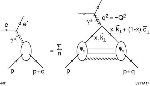
Figure 1: Calculation of the form factor of a bound state from the convolution of light-cone Fock amplitudes. The result is exact if one sums over all $\psi_{n}$.

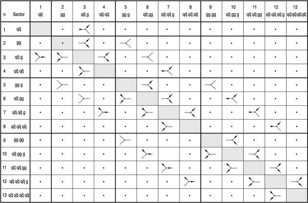
Figure 2: The Hamiltonian matrix for a meson. The matrix elements are represented by energy diagrams. Only vertex diagrams $V$ are shown. Zero matrices are marked by a dot ($\cdot$).

Let me sketch the method briefly. Details may be found in [6, 8]. DLCQ with its periodic boundary conditions has the advantage that the LC-Hamiltonian is a matrix with a finite number of Fock-space sectors, which we denumerate by $n$, with $1<n\leq N$. The so called harmonic resolution $K=LP^{+}/(2\pi)$ acts as a natural cut-off of the particle number. As shown in Figure 2, $K=3$ allows for $N=8$, and $K=4$ for $N=13$ Fock-space sectors, for example. The Hamiltonian matrix is sparse: Most of the matrix elements are zero, particularly if one includes only the vertex interaction $V$. For $n$ sectors, the eigenvalue problem in terms of block matrices reads

$$\sum_{j=1}^{n}\langle i|H_{n}(\omega)|j\rangle\langle j|\Psi(\omega)\rangle=E(\omega)\ \langle i|\Psi(\omega)\rangle,\qquad{\rm for}\ i=1,2,\dots,n.$$ (2)

I can always invert the quadratic block matrix of the Hamitonian in the last sector to define the $n$-space resolvent $G_{n}$, that is

$$G_{n}(\omega)={1\over\omega-H_{n}(\omega)}.$$ (3)

Using $G_{n}$, I can express the projection of the eigenfunction in the last sector by

$$\langle n|\Psi(\omega)\rangle=G_{n}(\omega)\sum_{j=1}^{n-1}\langle n|H_{n}(\omega)|j\rangle\ \langle j|\Psi(\omega)\rangle,$$ (4)

and substitute it in Eq.(2). I then get an effective Hamiltonian where the number is sectors is diminuished by 1:

$$H_{n-1}(\omega)=H_{n}(\omega)+H_{n}(\omega)G_{n}(\omega)H_{n}(\omega).$$ (5)

This is a recursion relation, which can repeated until one arrives at the $q\bar{q}$-space. The fixed point equation $E(\omega)=\omega$ determines then all eigenvalues.

For the block matrix structure as in Figure 2, with its many zero matrices, the reduction is particularly easy and transparent. For $K=3$ one has the following sequence of effective interactions:

$$H_{8}=T_{8},\quad H_{7}=T_{7}+VG_{8}V,\quad H_{6}=T_{6}+VG_{7}V,\quad H_{5}=T_{5}+VG_{6}V.$$ (6)

The remaining ones get more complicated, i.e.

$$H_{4} = T_{4}+VG_{7}V+VG_{7}VG_{6}VG_{7}V,$$ (7)

$$H_{3} = T_{3}+VG_{6}V+VG_{6}VG_{5}VG_{6}V+VG_{4}V,$$ (8)

$$H_{2} = T_{2}+VG_{3}V+VG_{5}V,$$ (9)

$$H_{1} = T_{1}+VG_{3}V+VG_{3}VG_{2}VG_{3}V.$$ (10)

For $K=4$, the effective interactions in Eq.(6) are different, see for example [8], but it is quite remarkable, that they are the same for the remainder, particularly Eq.(10). In fact, the effective interactions in sectors 1-4 are independent of $K$: The continuum limit $K\rightarrow\infty$ is then trivial, and will be taken in the sequel.

In the continuum limit, the effective interaction in the $q\bar{q}$-space has thus two contributions: A flavor-conserving piece $U_{\mathit{eff-conser}}=VG_{3}V$ and a flavor-changing piece $U_{\mathit{eff-change}}=VG_{3}VG_{2}VG_{3}V$. The latter cannot get active in flavor-off-diagonal mesons. Notice that these expressions are an exact result.

4 The eigenvalue equation in the $q\bar{q}$-space

After some approximations [6], the effective one-body equation for flavor off-diagonal mesons (mesons with a different flavor for quark and anti-quark), becomes quite simple:

$$M^{2}\langle x,\vec{k}_{\!\perp};\lambda_{1},\lambda_{2}|\psi\rangle=\left[\frac{\overline{m}^{2}_{1}+\vec{k}_{\!\perp}^{\,2}}{x}+\frac{\overline{m}^{2}_{2}+\vec{k}_{\!\perp}^{\,2}}{1-x}\right]\langle x,\vec{k}_{\!\perp};\lambda_{1},\lambda_{2}|\psi\rangle$$ (11)

$$-\frac{1}{3\pi^{2}}\sum_{\lambda_{q}^{\prime},\lambda_{2}^{\prime}}\!\int\frac{dx^{\prime}d^{2}\vec{k}_{\!\perp}^{\prime}\,R(x^{\prime},\vec{k}^{\prime}_{\!\perp};\Lambda)}{\sqrt{x(1-x)x^{\prime}(1-x^{\prime})}}\frac{\overline{\alpha}}{\,Q^{2}}\langle\lambda_{1},\lambda_{2}|S|\lambda_{1}^{\prime},\lambda_{2}^{\prime}\rangle\,\langle x^{\prime},\vec{k}_{\!\perp}^{\prime};\lambda_{1}^{\prime},\lambda_{2}^{\prime}|\psi\rangle.$$

Here, $M^{2}$ is the eigenvalue of the invariant-mass squared. The associated eigenfunction $\psi\equiv\Psi_{q\bar{q}}$ is the probability amplitude $\langle x,\vec{k}_{\!\perp};\lambda_{1},\lambda_{2}|\psi\rangle$ for finding a quark with momentum fraction $x$, transversal momentum $\vec{k}_{\!\perp}$ and helicity $\lambda_{1}$, and correspondingly the anti-quark with $1-x$, $-\vec{k}_{\!\perp}$ and $\lambda_{2}$. The $\overline{m}_{1}$ and $\overline{m}_{2}$ are (effective) quark masses and $\overline{\alpha}$ is the (effective) coupling constant. The mean Feynman-momentum transfer of the quarks is denoted by

$$Q^{2}\equiv Q^{2}(x,\vec{k}_{\!\perp};x^{\prime},\vec{k}_{\!\perp}^{\prime})=-\frac{1}{2}\left[(k_{1}-k_{1}^{\prime})^{2}+(k_{2}-k_{2}^{\prime})^{2}\right],$$ (12)

and the spinor factor $S=S(x,\vec{k}_{\!\perp};x^{\prime},\vec{k}_{\!\perp}^{\prime})$ by

$$\langle\lambda_{1},\lambda_{2}|S|\lambda_{1}^{\prime},\lambda_{2}^{\prime}\rangle=\left[\overline{u}(k_{1},\lambda_{1})\gamma^{\mu}u(k_{1}^{\prime},\lambda_{1}^{\prime})\right]\,\left[\overline{v}(k_{2}^{\prime},\lambda_{2}^{\prime})\gamma_{\mu}v(k_{2},\lambda_{2})\right].$$ (13)

The regulator function $R(x^{\prime},\vec{k}^{\prime}_{\!\perp};\Lambda)$ restricts the range of integration as function of some mass scale $\Lambda$. I happen to choose here a soft cut-off (see below), in contrast to the previous sharp cut-off [9]. Note that Eq.(11) is a fully relativistic equation. I have derived the same effective interaction also with the method of Hamiltonian flow equations, see [10].

The effective quark masses $\overline{m}_{1}$ and $\overline{m}_{2}$ and the effective coupling constant $\overline{\alpha}$ depend, in general, on $\Lambda$. In the spirit of renormalization theory they are renormalization constants, subject to be determined by experiment, and hence-forward will be denoted by $m_{1}$, $m_{2}$, and $\alpha$, respectively. In next-to-lowest order of approximation the coupling constant becomes a function of the momentum transfer, $\overline{\alpha}\longrightarrow\overline{\alpha}(Q;\Lambda)$, with the explicit expression given in [6].

5 The $\uparrow\downarrow$-model and its renormalization

It might be to early for solving Eq.(11) numerically in full glory like in Ref.[9]. Rather should I try to dismantle the equation of all irrelevant details, and develop a simple model.

The quarks are at relative rest, when $\vec{k}_{\!\perp}=0$ and $x=\overline{x}\equiv m_{1}/(m_{1}+m_{2})$. For very small deviations from these equilibrium values the spinor matrix is proportional to the unit matrix, with

$$\langle\lambda_{1},\lambda_{2}|S|\lambda_{1}^{\prime}\lambda_{2}^{\prime}\rangle\sim 4m_{1}m_{2}\ \delta_{\lambda_{1},\lambda_{1}^{\prime}}\ \delta_{\lambda_{2},\lambda_{2}^{\prime}},$$ (14)

for details see [10]. For very large deviations, particularly for $\vec{k}_{\!\perp}^{\prime\,2}\gg\vec{k}_{\!\perp}^{\,2}$, holds

$$Q^{2}\simeq\vec{k}_{\!\perp}^{\prime\,2},\hskip 20.00003pt\mbox{ and }\hskip 20.00003pt\langle\uparrow\downarrow|S|\uparrow\downarrow\rangle\simeq 2\vec{k}_{\!\perp}^{\prime\,2}.$$ (15)

Both extremes are combined in the “$\uparrow\downarrow$-model” [10]:

$$\frac{S}{Q^{2}}\equiv\frac{4m_{1}m_{2}}{Q^{2}}+2\Longrightarrow\frac{4m_{1}m_{2}}{Q^{2}}+2R(\Lambda,Q),\quad\textrm{with}\quad R(\Lambda,Q)=\frac{\Lambda^{2}}{\Lambda^{2}+Q^{2}}.$$ (16)

It interpolates between two extremes: For small momentum transfer, the ‘2’ generated by the hyperfine interaction is unimportant and the dominant Coulomb aspects of the first term prevail. For large momentum transfers the Coulomb aspects are unimportant and the hyperfine interaction dominates.

Figure 3: Nine contours $\alpha_{n}(\Lambda)$ are plotted versus $\Lambda/\Delta$, from bottom to top with $n=4,3,\cdots,-3,-4$. The contours are obtained by $M_{0}^{2}(\alpha,\Lambda)=n\Delta^{2}+M_{\pi}^{2}$. The thick contour $n=0$ refers to the pion with $M_{0}^{2}=M_{\pi}^{2}$. Mass unit is $\Delta=350$ MeV.

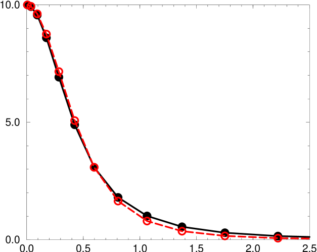
Figure 4: The pion wave function $\Phi(p)$ is plotted versus $p/(1.338m)$ in an arbitrary normalization. The filled circles indicate the numerical results, the open circles the analytical function $\Phi_{a}(p)$.

The model over-emphasizes many aspects: It neglects the momentum dependence of the Dirac spinors and thus the spin-orbit interaction; it also neglects the momentum dependence of the spin-spin interaction. But the 2 creates havoc: Its Fourier transform is a Dirac-delta function with all its consequences in a bound-state equation.

Here is an interesting point: One is familiar with field theoretic divergences like the effective masses and the effective coupling constant. One is used less to “divergences” residing in a finite number 2. They must be regulated also, and renormalized.

In consequence I replace Eq.(11) by

$$M^{2}\psi(x,\vec{k}_{\!\perp})=\left[\frac{m^{2}_{1}+\vec{k}_{\!\perp}^{\,2}}{x}+\frac{m^{2}_{2}+\vec{k}_{\!\perp}^{\,2}}{1-x}\right]\psi(x,\vec{k}_{\!\perp})$$

$$-\frac{\alpha}{3\pi^{2}}\!\int\frac{dx^{\prime}d^{2}\vec{k}_{\!\perp}^{\prime}}{\sqrt{x(1-x)x^{\prime}(1-x^{\prime})}}\left(\frac{4m_{1}m_{2}}{Q^{2}}+\frac{2\Lambda^{2}}{\Lambda^{2}+Q^{2}}\right)\psi(x^{\prime},\vec{k}_{\!\perp}^{\prime}),$$ (17)

where $\psi(x,\vec{k}_{\!\perp})\equiv\langle x,\vec{k}_{\!\perp};\uparrow,\downarrow|\psi\rangle$.

For equal quark masses $m_{1}=m_{2}=m$, the eigenvalues depend now on three parameters, the canonical $\alpha$ and $m$, and the regularization scale $\Lambda$. The dependence can be quite strong as seen in Figure 4. There, the lowest mass-squared eigenvalue is plotted versus $\alpha$ and $\Lambda$ for the fixed quark mass $m=406$ MeV.

Since $\Lambda$ is an unphysical parameter, its impact must be removed by renormalization. Recently, much progress was made on this question [11, 12]: Adding to $R(\Lambda,Q)$ a counterterm $C(\Lambda,Q)$ and requiring that the sum $\widetilde{R}(\Lambda,Q)=R(\Lambda,Q)+C(\Lambda,Q)$, and thus $M^{2}(\Lambda;\alpha,m)$, be independent of $\Lambda$, determines $C(\Lambda,Q)$. One remains with $\widetilde{R}(\Lambda,Q)=\mu^{2}/(\mu^{2}+Q^{2})$. In line with renormalization theory, one then can go to the limit $\Lambda\longrightarrow\infty$. In turn, $\mu$ becomes one of the parameters of the theory to be determined by experiment.

6 Determining the canonical parameters

The theory has seven canonical parameters which have to be determined by experiment: $\alpha$, $\mu$ and the 5 flavor masses $m_{f}$ (if we disregard the top). How can we determine them?

The problem is not completely trivial. Let me restrict first to the light flavors. With $m_{u}=m_{d}=m$, one has 3 parameters, and in consequence needs 3 experimental data. The pion mass $M_{\pi}=140$ MeV and the rho mass $M_{\rho}=768$ MeV do not suffice. One needs a third datum, the mass of an exited pion, for example.

Since the mass of the excited pion $\pi^{\pm}$ is not known with sufficient experimental precision, and since the $\uparrow\downarrow$-model might be to crude a model to begin with, I choose here $m_{u}=m_{d}=406$ MeV and $M_{\pi^{*}}=M_{\rho}=768$ MeV, for no good reason other than convenience. These assumptions are less stringent than they sound, by two reasons. First, the rho has a mass less than $2m$ and should be a true bound state. Second, the Yukawa potential in Eq.(17) acts like a Dirac-delta function in pairing theory for example: it pulls down essentially one state, the pion, but leaves the other states unchanged.

We thus remain with the two parameters $\alpha$ and $\mu$. Each of the two equations, $M_{0}^{2}(\alpha,\mu)=M_{\pi}^{2}$ and $M_{1}^{2}(\alpha,\mu)=M_{\pi^{*}}^{2}$ determine a function $\alpha(\mu)$. Their intersection point determines the required solution, which is $\alpha=0.761$ and $\mu=1.15$ GeV [11]. These differ marginally from the previous analysis [10], with $\mu=1.33$ GeV, for which Figure 4 yields $\alpha=0.6904$. Once I have the up and down mass, the strange, charm and bottom quark mass can be determined by reproducing the masses of the $K,^{-}$ $D^{0}$ and $B,^{-}$ respectively. The parameters in the $\uparrow\downarrow$-model can thus be taken as

$\alpha$	$\mu$	$m_{u}=m_{d}$	$m_{s}$	$m_{c}$	$m_{b}$
0.6904	1.33 GeV	406 MeV	508 MeV	1666 MeV	5054 MeV.

(I)

	$\overline{u}$	$\overline{d}$	$\overline{s}$	$\overline{c}$	$\overline{b}$
$u$		768	871	2030	5418
$d$	140		871	2030	5418
$s$	494	494		2124	5510
$c$	1865	1865	1929		6580
$b$	5279	5279	5338	6114

Table 1: The calculated mass eigenvalues in MeV. Those for singlet-1s states are given in the lower, those for singlet-2s states in the upper triangle.

	$\overline{u}$	$\overline{d}$	$\overline{s}$	$\overline{c}$	$\overline{b}$
$u$		768	892	2007	5325
$d$	140		896	2010	5325
$s$	494	498		2110	—
$c$	1865	1869	1969		—
$b$	5278	5279	5375	—

Table 2: Empirical masses of the flavor-off-diagonal physical mesons in MeV. Vector mesons are given in the upper, scalar mesons in the lower triangle.

7 The masses of the physical mesons

Solving Eq.(17) with the parameters of Eq.(I) generates the mass²-eigenvalues of all flavor off-diagonal pseudo-scalar mesons. They are compiled in Table 2. The corresponding wave functions are also available, but not shown here. In view of the simplicity of the model, the agreement with the empirical values [13] in Table 2 is remarkable. The mass of the first excited states in Table 2 correlates astoundingly well with the experimental mass of the pseudo-vector mesons, as given in Table 2. Notice that all numbers in Tables 2 and 2 are rounded for convenience.

Since the $\uparrow\downarrow$-model in Eq.(17) does not expose confinement one should emphasize that the difference between the physical meson masses in Table 2 amd the sum of the bare quark masses is larger than a pion mass. One could call this a kind of practical confinement.

	$M_{f\bar{f}}$	$M$	$M_{\mathrm{exp}}$
$\pi^{0}$	140	140	135
$\eta$	140	485	549
$\eta^{\prime}$	661	958	958
$\eta_{c}$	2870	2915	2980
$\eta_{b}$	8922	8935	—

Table 3: Flavor-diagonal mass eigenvalues in the FM-model for pseudo-scalar mesons with the parameter $a=(491\mbox{ MeV})^{2}$.

	$M_{f\bar{f}}$	$M$	$M_{\mathrm{exp}}$
$\rho^{0}$	768	768	768
$\omega$	768	832	782
$\Phi$	973	1019	1019
$J/\Psi$	3231	3242	3097
$\Upsilon$	9822	9825	9460

Table 4: Flavor-diagonal mass eigenvalues in the FM-model for pseudo-vector mesons with the parameter $a=(255\mbox{ MeV})^{2}$.

What about the flavor diagonal mesons?– They cannot be a solution to Eqs.(11) or (17), since the flavor-changing piece of the full effective interaction can generate matrix elements between different flavors. Thus far the precise structure of the flavor changing part $U_{\mathit{eff-change}}=VG_{3}VG_{2}VG_{3}V$ has not been analyzed in detail, because it requires a considerable effort.

Rather, the following flavor-mixing model (FM-model [15]) has been investigated. In the FM-model, the full effective Hamiltonian including its flavor mixing is reduced to the lowest $f\bar{f}$-states, i.e. to

$$\langle f\bar{f}|H_{\mathit{eff}}|f^{\prime}\bar{f}^{\prime}\rangle=\langle\psi_{f\bar{f}}|T+VG_{3}V+VG_{3}VG_{2}VG_{3}V|\psi_{f^{\prime}\bar{f}^{\prime}}\rangle=M_{ff^{\prime}}^{2}\ \delta_{ff^{\prime}}+a.$$ (18)

Conceptually, it is important that $M_{ff^{\prime}}^{2}$ is the eigenvalue of Eq.(17). The flavor-mixing matrix element $a=\langle\psi_{f\bar{f}}|VG_{3}VG_{2}VG_{3}V|\psi_{f^{\prime}\bar{f}^{\prime}}\rangle$ depends on the flavors and could be calculated with a solution of Eqs.(11) or (17). In the crude FM-model, however, it is treated as a flavor-independent parameter to be fixed by experiment. For 5 flavors one faces thus the numerical diagonalization of a $5\times 5$ matrix.

The parameter $a$ for pseudo-scalar mesons was fitted to the mass of the $\eta^{\prime}$, and for pseudo-vector mesons to the $\Phi$, with the results compiled in Tables 4 and 4 . Three facts, however, one gets for free: First, the $\pi^{0}$ is degenerate in mass with $\pi^{\pm}$, as well as the $\rho^{0}$ with $\rho^{\pm}$. That they form isospin-triplets is a non-trivial aspect of QCD. Second, both the $\eta$–$\eta^{\prime}$ and the $\omega$–$\Phi$ splitting are in the right bull park. Third, that the wave functions of the $\pi^{0},\eta$ and $\eta^{\prime}$ have very much SU(3)-character [15] is even less trivial from the point of view of QCD.

8 The wavefunction of the pion

For carrying out this programme in practice, I need an efficient tool for solving Eq.(17). Such one has been developed recently [10]. I outline in short the procedure for the special case $m_{1}=m_{2}=m$. I change integration variables from $x$ to $k_{z}$ by substituting

$$x(k_{z})=\frac{1}{2}+\frac{k_{z}}{2\sqrt{m^{2}+\vec{k}_{\!\perp}^{\,2}+k_{z}^{2}}},\hskip 30.00005pt\psi(x,\vec{k}_{\!\perp})=\frac{\sqrt{1+(\vec{k}_{\!\perp}^{\,2}+k_{z}^{2})/m^{2}}}{\sqrt{x(1-x)}}\ \phi(k_{z},\vec{k}_{\!\perp}).$$ (19)

The variables $(k_{z},\vec{k}_{\!\perp})$ are collected in a 3-vector $\vec{p}$ and Eq.(17) becomes

$$\left[M^{2}-4m^{2}-4\vec{p}^{\,2}\right]\phi(\vec{p}) = -\frac{4\alpha}{3\pi^{2}}\int\!\!d^{3}\vec{p}\,^{\prime}\left(\frac{2m}{(\vec{p}-\vec{p}\,^{\prime})^{\,2}}+\frac{1}{m}\frac{\mu^{2}}{\mu^{2}+(\vec{p}-\vec{p}\,^{\prime})^{2}}\right)\phi(\vec{p}\,^{\prime}).$$ (20)

For the present purpose it suffices to restrict to spherically symmetric $s$-states $\phi(\vec{p})=\phi(p)$ and to apply Gaussian quadratures with 16 points. On an alpha work station it takes a couple of micro-seconds to solve this equation for a particular case. The resulting numerical wavefunction $\phi(p)$ is displayed in Figure 4 and compared with

$$\Phi_{a}(p)=\mathcal{N}\left(1+\displaystyle\frac{p^{2}}{p_{a}^{2}}\right)^{-2},\hskip 30.00005pt\mathrm{with}\quad p_{a}=1.338\ m.$$ (21)

Such an analytical form is convenient in many applications. For example, the light-cone wavefunction $\psi(x,\vec{k}_{\!\perp})$ can be obtained in closed form by Eq.(19), i.e.

$$\psi(x,\vec{k}_{\!\perp})=\frac{\mathcal{N}}{\sqrt{x(1-x)}}\frac{\left(1+\displaystyle\frac{m^{2}\left(2x-1\right)^{2}+\vec{k}_{\!\perp}^{\,2}}{4x(1-x)\ m^{2}}\right)^{\frac{1}{2}}}{\left(1+\displaystyle\frac{m^{2}\left(2x-1\right)^{2}+\vec{k}_{\!\perp}^{\,2}}{4x(1-x)\ p_{a}^{2}}\right)^{2}}.$$ (22)

I can use this to calculate the form factor from Eq.(1), and thus the exact root-mean-square radius [14], even in closed form with $\langle r^{2}\rangle=-6\left.{dF_{2}(Q^{2})}/{dQ^{2}}\right|_{Q^{2}=0}$:

$$\langle r^{2}\rangle = \frac{3}{4p_{a}^{2}}\ \frac{34+37s^{2}-41s^{4}+15s^{6}+3b(s)(-8-16s^{2}+21s^{4}-17s^{6}+5s^{8})}{5(s^{2}-1)[4-4s^{2}+3s^{4}+3b(s)s^{4}(-2+s^{2})]},$$ (23)

with $s={m}/{p_{a}}$ and the abbreviation $b(s)=\mathrm{arctan}(\sqrt{s^{2}-1})/\sqrt{s^{2}-1}$. The size of the $q\bar{q}$ wavefunction is thus $\langle r^{2}\rangle^{\frac{1}{2}}=0.33$ fm, half as large as the empirical value $\langle r^{2}\rangle_{\mathrm{exp}}^{\frac{1}{2}}=0.67$ fm.

This completes the goal: I have a pion with the correct mass, and I have an analytic expression for its light-cone wave function. Eq.(22) could be used thus as a baseline for calculating the higher Fock-space amplitudes, as explained in [8].

It might well be that the wavefunction in Eq.(22) is consistent with Ashery’s experiment [16].

9 Conclusions

The proposed pion of the $\uparrow\downarrow$-model is rather different from the pions in the literature. I have found no evidence that the vacuum condensates are important, but I conclude that the pion is describable by a QCD-inspired theory: The very large coupling constant in conjunction with a very strong hyperfine interaction makes it a ultra strongly bounded system of constituent quarks. More then 80 percent of the constituent quark mass is eaten up by binding effects. No other physical system has such a property.

The effective Bohr momentum of the constituents in the pion turns out as $p_{a}=1.338\,m$, see Eq.(21). The mean momentum of the constituents is thus 40 percent larger than their mass, which means that they move highly relativistically quite in contrast with the constituents of atoms or nuclei. No wonder that potential models thus far have failed for the pion. One might mention that lattice gauge calculations use all the computer power in this world to generate the potential energy of the quarks and then one uses a non-relativistic Schrödinger equation to calculate the bound states.

All this is to be confronted with the present oversimplified $\uparrow\downarrow$-model, which however has the virtue to calculate the pion and other physical mesons by a covariant and relativistically correct theory. To the best of my knowledge there is no other model which can describe all mesons quantitatively from the $\pi$ up to the $\Upsilon$ from a common point of view, which here is QCD.

References

- [1] G. Schierholz, Nucl. Phys. Proc. Suppl. 90 (2000) 207.
- [2] K. Schilling, Nucl. Phys. Proc. Suppl. 83 (2000) 140.
- [3] W. Plessas, these proceedings.
- [4] H. Leutwyler, Workshop on LC-Physics, Trento, Sep 2001.
- [5] S.J. Brodsky, H.C. Pauli, and S.S. Pinsky, Phys. Rep. 301 (1998) 299-486.
- [6] H.C. Pauli, Eur. Phys. J. C7 (1998) 289. hep-th/9809005.
- [7] J. Hiller, Nucl. Phys. Proc. Suppl. 90 (2000) 170.
- [8] H.C. Pauli, in: New directions in Quantum Chromodynamics, C.R. Ji and D.P. Min, Eds., American Institute of Physics, 1999, p. 80-139. hep-ph/9910203.
- [9] U. Trittmann and H.C. Pauli, Nucl. Phys. Proc. Suppl. 90 (2000) 161.
- [10] H.C. Pauli, Nucl. Phys. B (Proc. Suppl.) 90 (2000) 147, 259.
- [11] M. Frewer et al., Workshop on LC-Physics, Trento, Sep 2001.
- [12] T. Frederico, M. Frewer, and H.C. Pauli Workshop on LC-Physics, Trento, Sep 2001. hep-ph/0111039
- [13] C. Caso et al., Eur.Phys.J. C3 (1998) 1.
- [14] H.C. Pauli, and A. Mukherjee, to appear in Int.Jour.Mod.Phys. (2001), hep-ph/0104175. H.C. Pauli, Submitted to Nucl.Phys. A(2001), hep-ph/0107302.
- [15] H.C. Pauli, Submitted to Nucl.Phys. A(2001), hep-ph/0103254.
- [16] D. Ashery, Nucl. Phys. Proc. Suppl. 90 (2000) 67.