Prospects for Searching for Excited Leptons during Run II of the Fermilab Tevatron

Abstract

This letter presents a study of prospects of searching for excited leptons during Run II of the Fermilab Tevatron. We concentrate on single and pair production of excited electrons in the photonic decay channel in one CDF/D$\O$ detector equivalent for 2 fb^-1. By the end of Run IIa, the limits should be easily extended beyond those set by LEP and HERA for excited leptons with mass above about 190 GeV.

E. Boos¹, A. Vologdin¹, D. Toback², and J. Gaspard<sup>2

1</sup>Institute of Nuclear Physics, Moscow State University, 119899, Moscow, Russia
²Texas A&M University, College Station, TX 77843 USA

The Standard Model (SM) of particle physics is known to give results that match the current experimental data with a high precision. However, because of well known theoretical problems and disadvantages, it is widely believed it can not be a complete theory of elementary particles, but rather, likely a kind of effective theory at energies below some scale of the order of a TeV. While many models of “new physics” beyond the SM have been suggested over the years, one of the most straight-forward ideas proposes that quarks and leptons are composite particles. Such a scenario is a recurring theme in nature; molecules are composed of atoms, which are in turn composed of nuclei, which are in turn composed of nucleons and so on. Furthermore, composite models can explain, in principle, family replication, mixing in the quark and lepton sectors, and even make the fermion masses and weak mixing angles calculable.

In most composite models fermions possess an underlying substructure which is characterized by a scale $\Lambda$ [1] with $\Lambda$ about 1 TeV or higher [2]. While there is no unified model of compositeness, a model-independent effective Lagrangian for excited leptons, originally proposed in [3], can be used to model single and pair production in experiments. The Lagrangian:

$$L_{l^{*}l^{*}} = \overline{l}^{*}\gamma^{\mu}(\frac{\tau}{2}W_{\mu}+g^{{}^{\prime}}\frac{Y}{2}B_{\mu})l^{*}$$ (1)

$$L_{l^{*}l} = \frac{1}{2\Lambda}\overline{l}^{*}_{R}\sigma^{\mu\nu}(fg\frac{\tau}{2}W_{\mu\nu}+f^{{}^{\prime}}g^{{}^{\prime}}\frac{Y}{2}B_{\mu\nu})l_{L}+h.c.$$ (2)

where $f$ and $f^{\prime}$ are coupling constants, has been used extensively in a number of phenomenological papers which presents ideas on searching for excited fermion production and decay to final state gauge bosons in $e^{+}e^{-}$, $p\bar{p}$, $ep$, and $e\gamma$ collisions [4, 5, 6]. Direct searches for lepton compositeness has been done extensively at LEP [7] and HERA [8], each with no discovery, but with ever more sensitive limits. Unfortunately, only direct searches for quark compositeness have been done at the Fermilab Tevatron [9].

In this Letter we present a study for searching for excited lepton production and decay for the upcoming Run II of CDF and D$\O$ detectors. We begin with an updated simulation of excited lepton production, and optimize the sensitivity by studying the kinematics of excited lepton production and decay. With these results we estimate the mass reach and compare to the recent results from LEP and HERA.

To study the mass reach of the Tevatron, we simulated single and pair production and decay of excited leptons using the upgraded Fermilab accelerator (1.8 $\rightarrow$ 2.0 TeV), and CDF and D$\O$ detectors for Run II. The Feynman rules from the effective Lagrangian (Eqn. 1) are implemented into CompHEP [10] using the LanHEP [11] software package. We have included into this simulation a complete tree-level calculation which takes into account all the spin correlations between excited states production, subsequent decays, and incorporate the known NLO corrections. All the partial width and known 2$\rightarrow$ 2 cross-section have been cross-checked at the symbolic level. Events on parton level generated by means of CompHEP have been used as an external process for pythia with the help of the CompHEP-pythia interface [12]. The underlying event, jet fragmentation, ISR and FSR are modeled using the pythia [13] Monte Carlo with the cteq4l [14] structure functions. Since Drell-Yan production of excited leptons production is similar to that of Supersymmetric leptons, we take the K-factors given in [15], which only depend on the masses of final particles, and vary between 1.23 and 1.24 in the mass range of the search.

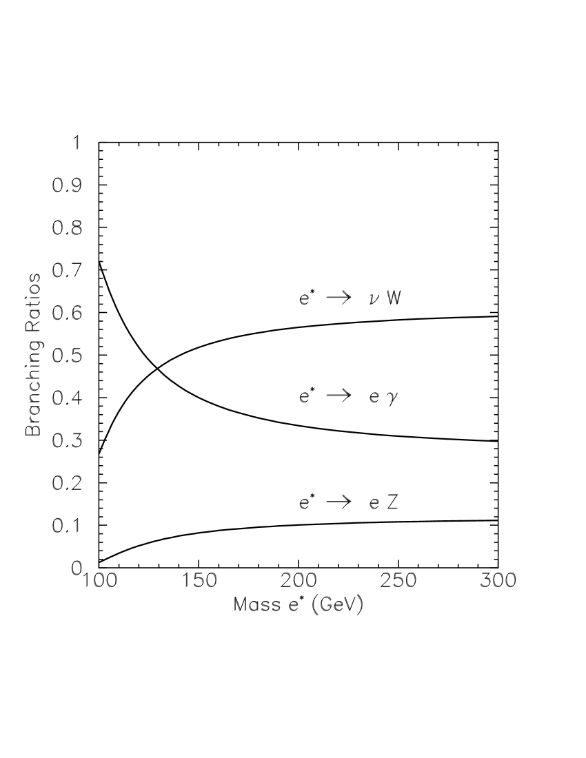
Figure 1: The branching ratios for excited leptons as a function of the mass of the excited lepton.

While excited leptons can come in three flavors: $e^{*}$, $\mu^{*}$ and $\tau^{*}$, we chose to concentrate on the electron since the result of $\mu^{*}$ expected to be similar to $e^{*}$, and $\tau$’s at the Tevatron are still difficult to trigger on and identify. Excited electrons can decay via: $e^{*}\rightarrow e\gamma$, $e^{*}\rightarrow eZ$, and $e^{*}\rightarrow W\nu$ channels with the branching ratios shown in Fig. 1. The backgrounds to the $W$ and $Z$ decay channels in the hadronic channels are fairly large and the leptonic branching fractions needed to identify the $W$ and $Z$ channels are small; however, the backgrounds to the photonic final states are relatively small in comparison making them a gold-plated signature.

In the case of the single excited electron production mode, there are two possible signal $p\overline{p}\rightarrow e^{*}e\rightarrow e^{+}e^{-}\gamma$ and $p\overline{p}\rightarrow e^{*}\nu\rightarrow e\nu\gamma$. Similarly, pair production gives $p\overline{p}\rightarrow e^{*+}e^{*-}\rightarrow e^{+}e^{-}\gamma\gamma$ and $p\overline{p}\rightarrow e^{*}\nu^{*}\rightarrow e\nu\gamma\gamma$. For simplicity we concentrate on inclusive $ee\gamma$ final state for both single and pair production as it covers most of the production in both single and pair production cases. Before taking into account the branching ratio to photons, the total production cross section is shown in Fig. 2 for the case $f/\Lambda=10^{-2}~{}{\rm GeV}^{-1}$ and $f=f^{{}^{\prime}}$.

There are a number of backgrounds to the $ee\gamma$ channel. The dominant backgrounds are $W\gamma$+jets and $Z\gamma$+jets production. Others include $W$+jets and $Z$+jets, and multijets, where jets can fake leptons and/or photons. Studies have shown [16] that the fake backgrounds can be modeled by the kinematics of the irreducible backgrounds. The backgrounds are modeled using the same CompHEP simulation structure described above. Since there is an infrared singularity at $p_{T}^{\gamma}=0$, we require $P_{T}^{\gamma}>10$ GeV and $\Delta R_{ij}>0.1$, where $\Delta R_{ij}\equiv\sqrt{(\Delta\eta)^{2}+(\Delta\varphi)^{2}}$, and at the generator level, $i$ and $j$ are any lepton-photon combination. We take the K-factor, which has a value of about 1.36 depending on $p_{T}^{\gamma}$, for the background processes from the literature [17].

For both signal and backgrounds, we use a parametric simulation to model the detector response. The SHW detector simulation [18] has been shown to be an effective averaging between the CDF [19] and DØ [20] detectors for Run II. After detector simulation the kinematic distributions for both the signal and estimated backgrounds are shown in Figs 3 and 4. We find acceptances at about the 0.3 level for signal.

To maximize our sensitivity we assume, for simplicity, that taking a set of cuts which minimizes the expected cross section limit also maximizes our sensitivity to calculate these limits. To calculate these limits, we use the signal acceptance and background estimates from the simulations above. We add in a single detector with 2 fb^-1 of luminosity and we assume the experimental parameters of Table 1 for systematic uncertainties. We use a frequentist method [21] to incorporate the errors and assume that all errors on acceptance, background and luminosity are uncorrelated. To determine the expected limit as a function of a given cut using Run II data, under the assumption of no observed signal, the 95% confidence level (C.L.) cross section upper limit, for a given cut, is uniquely determined by number of events observed in the data. With no signal, the number of events observed in the data, $N$, fluctuates around the mean number of expected events, $M$, according to Poisson statistics. Thus, an average expected cross section limit is given by:

$$\sigma_{95}^{cut}=\sum_{N=0}^{\infty}\sigma_{95}(N,cut)\frac{e^{-M}M^{N}}{N!}$$ (3)

Luminosity (fb-1)	2.0 $\pm$ 0.1
Background error $\frac{\delta N_{back}}{N_{back}}$	0.1
Acceptance error $\frac{\delta A}{A}$	0.1

Table 1: Parameters used to calculate the 95% C.L. cross section upper limits.

In this way we get an average expected cross section limits as a function of each cut. We can then optimize for each mass point as a function of the cuts.

After a study of multi-dimensional distributions for background and signal, we determined that the $e^{+}e^{-}\gamma$ final state has the best signal to background ratio and kinematical distributions. Furthermore, we find that applying a single cut on the kinematical variable $M_{e\gamma}$ (where $e$ is the electron with highest $p_{T}$) gives the best relation between acceptance and $N$ to find minimal value of $\sigma_{95}$ for a given mass of the excited electron. This is readily apparent using Figs. 3 and 4 which shows that the best separation between signal and background is the $M_{e\gamma}$ variable.

$M_{e^{*}}$	$\sigma^{prod}$	$\cal B$ ($e^{*}\rightarrow e\gamma$)	Cut	Nback	$\sigma_{\rm 95\%~{}C.L}^{expected}$	$\sigma_{\rm 95\%~{}C.L}^{expected}\cdot\cal B$
(GeV)	(fb)		(GeV)		(fb)	(fb)
150	712	0.400	140.0	42.0	41.3	16.5
200	312	0.334	185.0	18.0	30.9	10.3
250	160	0.309	230.0	7.64	23.7	7.3
300	87	0.297	275.0	4.36	20.0	5.9

Table 2: Values for $\frac{f}{\Lambda}$ = $\frac{1}{100}$ GeV^-1 optimized points.

Figure 5 shows the expected 95% C.L. cross section upper limit, $\sigma_{95}$, as a function of the $M_{e\gamma}$ cut for different masses of $e^{*}$ for $\frac{f}{\Lambda}$ = $\frac{1}{100}$ GeV^-1. Placing our cut at the minimum of the curve gives our optimization, and final expected cross section limit. These results are shown in Fig. 6. Using the Feynman rules for the Lagrangian in Eqn. 1 leads to a simple relation between cross-section and $\frac{f}{\Lambda}$ for signal:

$$(\Lambda_{1})^{2}\sigma(\frac{f}{\Lambda_{1}},M_{e^{*}})=(\Lambda_{2})^{2}\sigma(\frac{f}{\Lambda_{2}},M_{e^{*}})$$ (4)

$$\frac{f}{\Lambda}=\frac{\sigma_{95}}{10^{4}\sigma(10^{-2},M_{e^{*}})}$$ (5)

Taking into account this equation, numerical values of signal cross-sections (where $\frac{f}{\Lambda}=10^{-2}$ GeV^-1) and results for $\sigma_{95}$ we can make an exclusion plot in the $\frac{f}{\Lambda}$ vs. $M_{e^{*}}$ plane. This result is shown in Fig. 7. We compare our results to those of LEP and HERA in Fig. 8 which would give the most stringent limits, to date, for masses above 190 GeV.

The prospects for searching for excited electrons at the upgraded Fermilab Tevatron are excellent. We expect that with a single detector and 2 fb^-1 of data should significantly extend the mass reach, especially in the low $\frac{f}{\Lambda}$ region and large masses. We also point out that similar results are obtained for excited muons which significantly improve on the current limits which are not producible at HERA.

The authors would like to thank John Hobbs for the use of his limit calculator, Bruce Knuteson for his relation in Eqn. 3, and Bhaskar Dutta for helpful discussions. We would also like to thank the D$\O$ collaboration for the use of their computers to do the simulation work. We also would like to thanks the Institute of Nuclear Physics of Moscow State University, the University of Maryland and Texas A&M University for their support. Finally we would like to thank the US DOE and Russian Ministry of Industry, Science and Technology for their support during this project. The work of E.B. and A.V. was partly supported by the RFBR-DFG 99-02-04011, RFBR 00-01-00704, CERN-INTAS 99-377, and Universities of Russia 990588 grants.

Figure 2: Total cross section for the sum of both single and pair production and decay of excited electrons in the $ee\gamma$ final state.

Figure 3: A comparison of the kinematic distributions of the final state electrons and photons for excited electron and standard model background processes. The figures show the results for single and pair production of ${e^{*}}e\rightarrow ee\gamma$ and ${e^{*}}{e^{*}}\rightarrow ee\gamma$.

Figure 4: A comparison of some of the variables studied which gave good separation between excited leptons and standard model background processes in the $ee\gamma$ final state. Note that the $M_{e\gamma}$ variable gives the best separation between signal and background for $M_{e^{*}}=200$ GeV at $M_{e\gamma}>185$ GeV.

Figure 5: The expected 95% C.L. cross section upper limit as a function of the $M_{e\gamma}$ cut for different masses of $e^{*}$. There the cross section is defined as $\sigma(p\bar{p}\rightarrow ee^{*}\rightarrow ee\gamma)$ + $\sigma(p\bar{p}\rightarrow e^{*}e^{*}\rightarrow ee\gamma)$ and $\mathcal{L}$ = 2 fb^-1.

Figure 6: Optimized expected 95% C.L. for $e^{*}\rightarrow ee\gamma$ production using the $ee\gamma$ final state and 2 fb^-1 of data with a single detector.

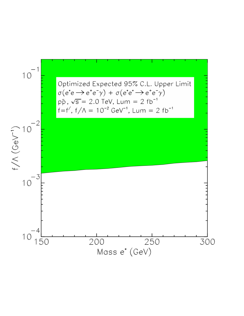
Figure 7: Exclusion plot for $\frac{f}{\Lambda}$ as a function of $e^{*}$ mass using 2 fb^-1 worth of data and a single detector.

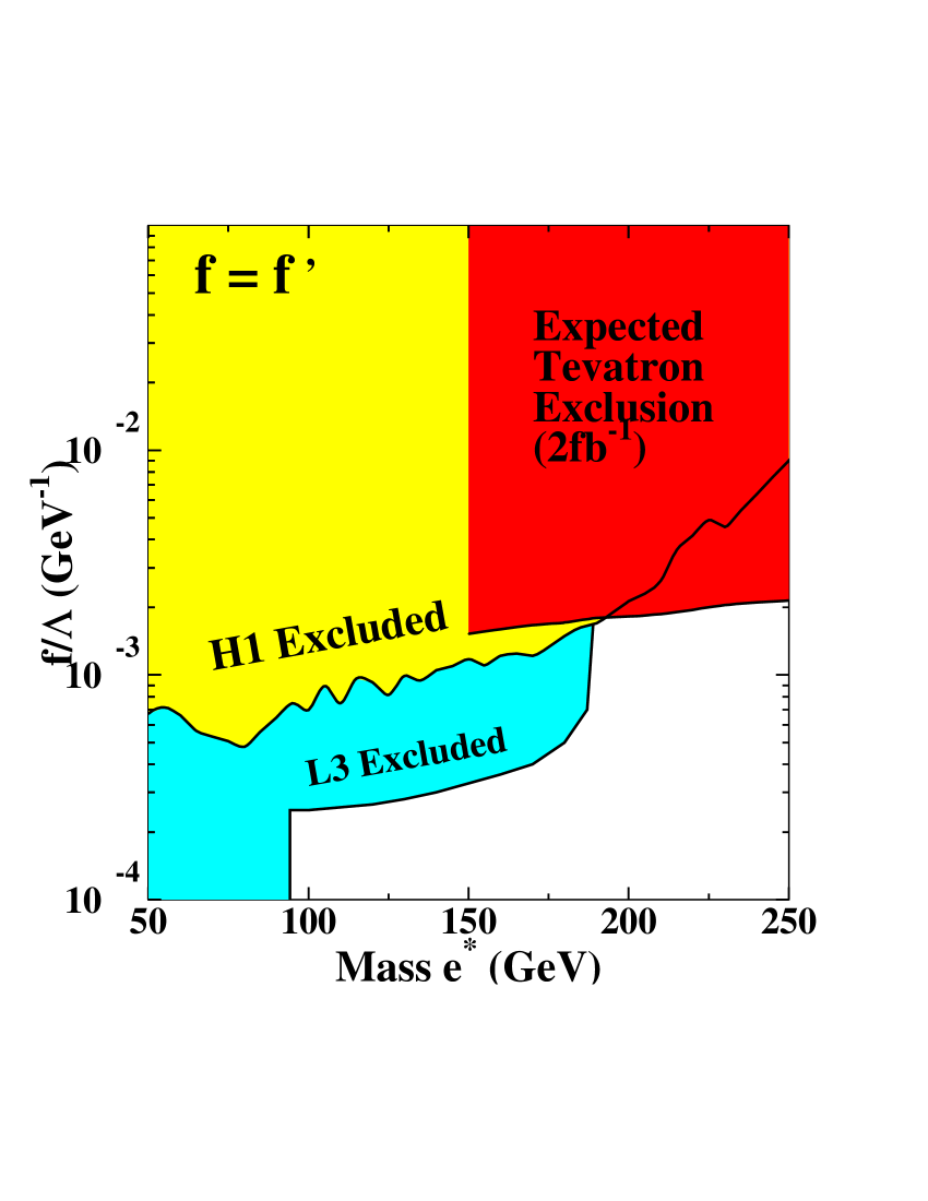
Figure 8: For masses above about 190 GeV, we expect that the Tevatron should, with 2 fb^-1 of data, and one detector, produce the most stringent limits.

References

- [1] On the other hand an existence of the excited states may be a results of a presence of extra dimensions. This may occur if the quark, lepton and boson fields can propagate in extra dimensions. However in that case one would expect an appearance of excited states in pairs as discussed in T. Appelquist, H. Cheng and B. A. Dobrescu, Phys. Rev. D 64, 035002 (2001).
- [2] Current experimental constraints come from the analysis of the properties of muon and electron, and from the estimate of quark and lepton radii. See A. Czarnecki, W. J. Marciano, [hep-ph/0010194], talk given at the Fifth International Symposium on Radiative Corrections (RADCOR 2000), Carmel, CA, September 2000; K. Lane, [hep-ph/01022131].
- [3] K. Hagiwara et al., Z. Phys. C 29, 115 (1985).
- [4] F. Boudjema et al., Z. Phys. C 57, 425 (1993).
- [5] U. Baur et al., Phys. Rev. D 42, 815 (1990).
- [6] E. Boos et al., Nucl. Phys. V 56, 5 (1993).
- [7] L3 Collaboration, M. Acciarri et al., Phys. Lett. B 473, 177 (2000); ALEPH Collaboration, D. Decamp et al., Phys. Lett. B 236, 501 (1990); ALEPH Collaboration, D. Buskulic et al., Phys. Lett. B 385, 445 (1996).
- [8] ZEUS Collaboration, M. Derrick et al., Phys. Lett. B 316, 207 (1993); ZEUS Collaboration, M. Derrick et al., Z. Phys. C 65, 627 (1995); ZEUS Collaboration, J. Breitweg et al., Z. Phys. C 76, 631 (1997); H1 Collaboration, C. Adloff et al., Eur. Phys. J. C17, 567 (2000); H1 Collaboration, S. Aid et al., Nucl. Phys. B 483, 44 (1997); H1 Collaboration, T. Ahmed et al., Phys. Lett. B 340, 205 (1994)
- [9] D Collaboration, B. Abbott et al., Phys. Rev. Lett. 82, 2457 (1999); D Collaboration, B. Abbott et al., Phys. Rev. Lett. 80, 666 (1998); D Collaboration, B. Abbott et al., Phys. Rev. D 62, 031101 (2000); CDF Collaboration, F. Abe et al., Phys. Rev. Lett. 71, 2542 (1993).
- [10] E. E. Boos et al., hep-ph/9503280, P. Baikov et al., Workshop on High Energy Physics and Quantum Field Theory, ed. by B. Levtchenko and V. Savrin, Moscow, 1996, 101; A. Pukhov et al., hep-ph/9908288.
- [11] A. Semenov, Nucl. Instrum. Methods A 393, 293 (1997); hep-ph 9608488.
- [12] A. S. Belyaev et al., hep-ph/0101232, To appear in the proceedings of the Seventh International Workshop on Advanced Computing and Analysis Technics in Physics Research (ACAT2000, Fermilab, October 16-20, 2000).
- [13] T. Sjöstrand, Comp. Phys. Comm. 82, 74 (1994); S. Mrenna, Computer Phys. Commun. 101, 232 (1997); T. Sjöstrand, P. Eden, C. Friberg, L. Lonnblad, G. Miu, S. Mrenna and E. Norrbin, Comp. Phys. Comm. 135, 238 (2001).
- [14] H. L. Lai et al.. Phys. Rev. D 55, 1280 (1997).
- [15] H. Baer et al., Phys. Rev. D 57, 5871 (1998).
- [16] D Collaboration, F. Abachi et al., Phys. Rev. Lett. 75, 1023 (1995).
- [17] J. Smith et al., Z. Phys. C 44, 267 (1989).
- [18] The Supersymmetry/Higgs Workshop, Version 2.3, Fermilab, Batavia IL, November 19, 1998. http://fnth37.fnal.gov/susy.html
- [19] CDF Collaboration, F. Abe et al., Nucl. Instrum. Methods A 271, 387 (1988).
- [20] D Collaboration, F. Abachi et al., Nucl. Instrum. Methods A 338, 185 (1994).
- [21] G. Zech, Nucl. Instrum. Methods A 227, 608 (1989); T. Huber et al., Phys. Rev. D 41, 2709 (1990).