Models with Extra Dimensions
and Their Phenomenology

Abstract

The Arkani-Hamed-Dimopoulos-Dvali and the Randall-Sundrum models with extra spacelike dimensions, recently proposed as a solution to the hierarchy problem, are reviewed. We discuss their basic properties and phenomenological effects of particle interactions at high energies, predicted within these models.

1 Introduction

Studies of field theoretical models in the space-time with additional spatial dimensions were started by T. Kaluza and O. Klein in their pioneering articles [1], [2] in the 20th. This gave the origin to a field theoretical approach to the description of particle interactions in a multidimensional space-time called the Kaluza-Klein (KK) approach.

Very detailed studies of various mathematical and physical aspects of models within the KK approach were carried out in the literature, see Refs. [3] - [5] for reviews and references therein. A strong motivation for the KK approach comes from the string theory where the multidimensionality of the space-time is required for the consistent formulation.

Recently models with extra dimensions of a new type, namely the Arkani-Hamed-Dimopoulos-Dvali (ADD) and Randall-Sundrum (RS) models, have been proposed in Refs. [6] - [9]. They were designed to provide a novel solution to the hierarchy problem. Many essential features of these models were inherited from the KK approach. Also many ideas and concepts, recently discovered in string/M-theories, have been incorporated. The ADD and RS models are the subject of the present contribution.

In the rest of this section we discuss main elements of the ”classical” KK theories. We also introduce the notion of localization of fields on branes by considering a simple model and mention briefly some recent results in string theories which serve as motivations for the ADD and RS models. Sect. 2 and Sect. 3 are devoted to the ADD model and the RS1 model respectively. We explain the basics of the models and discuss possible effects, predicted by them, which can be observed in high energy particle experiments. We almost do not touch astrophysical effects and cosmological scenarios within the ADD and RS models restricting ourselves to a very general discussion and brief remarks. Sect. 4 contains a short summary of results on the ADD and RS1 models.

In the present account we follow mainly the original papers on the subject and some recent reviews, Refs. [10] - [13].

1.1 Kaluza-Klein approach

The KK approach is based on the hypothesis that the space-time is a $(4+d)$-dimensional pseudo-Euclidean space

$$E_{4+d}=M_{4}\times K_{d},$$ (1)

where $M_{4}$ is the four-dimensional space-time and $K_{d}$ is a $d$-dimensional compact space of characteristic size (scale) $R$. The latter plays the role of the space of additional (spatial) dimensions of the space-time. Let us denote local coordinates of $E_{4+d}$ as $\{\hat{x}^{M}\}=\{x^{\mu},y^{m}\}$, where $M=0,1,\ldots,3+d$, $\mu=0,1,2,3$ and $m=1,2,\ldots,d$. In accordance with the direct product structure of the space-time, Eq. (1), the metric is usually chosen to be

$$ds^{2}=\hat{G}_{MN}(\hat{x})d\hat{x}^{M}d\hat{x}^{N}=g_{\mu\nu}(x)dx^{\mu}dx^{\nu}+\gamma_{mn}(x,y)dy^{m}dy^{n}.$$

To illustrate main elements and ideas of the KK approach which will be important for us later, let us consider the case of $M_{4}=M^{4}$, the Minkowski space-time, and a simple $(4+d)$-dimensional scalar model with the action given by

$$S=\int d^{4+d}\hat{x}\sqrt{-\hat{G}}\left[-\frac{1}{2}\left(\partial_{M}\hat{\phi}\right)^{2}-\frac{m^{2}}{2}\hat{\phi}^{2}-\frac{g_{(4+d)}}{4!}\hat{\phi}^{4}\right],$$ (2)

where $\hat{G}=\det(\hat{G}_{MN})$. To interprete the theory as an effective four-dimensional one the multidimensional field $\hat{\phi}(x,y)$ is expanded in a Fourier series

$$\hat{\phi}(x,y)=\sum_{n}\phi^{(n)}(x)Y_{n}(y),$$ (3)

where $Y_{n}(y)$ are orthogonal normalized eigenfunctions of the Laplace operator $\Delta_{K_{d}}$ on the internal space $K_{d}$,

$$\Delta_{K_{d}}Y_{n}(y)=\frac{\lambda_{n}}{R^{2}}Y_{n}(y),$$ (4)

and $n$ is a (multi-) index labeling the eigenvalue $\lambda_{n}$ of the eigenfunction $Y_{n}(y)$.

The case of the toroidal compactification of the space of extra dimensions $K_{d}=T^{d}$, where $T^{d}$ denotes the $d$-dimensional torus with equal radii $R$, is particularly simple. The multi-index $n=\{n_{1},n_{2},\ldots,n_{d}\}$ with $n_{m}$ being integer numbers, $-\infty\leq n_{m}\leq\infty$. The eigenfunctions and eigenvalues in Eqs. (3), (4) are given by

$$Y_{\{n_{1},n_{2},\ldots n_{d}\}} = \frac{1}{\sqrt{V_{d}}}\exp\left\{\frac{i\sum_{m=1}^{d}n_{m}y^{m}}{R}\right\},$$ (5)

$$\lambda_{\{n_{1},n_{2},\ldots n_{d}\}} = n_{1}^{2}+n_{2}^{2}+\ldots n_{d}^{2},$$

where $V_{(d)}=(2\pi R)^{d}$ is the volume of the torus.

The coefficients $\phi^{(n)}(x)$ of the Fourier expansion (3) are called KK modes and play the role of fields of the effective four-dimensional theory. Usually they include the zero-mode $\phi^{(0)}(x)$, corresponding to $n=0$ and the eigenvalue $\lambda_{0}=0$. Substituting the KK mode expansion into action (2) and integrating over the internal space $K_{d}$ one gets

$$S = \int d^{4}x\sqrt{-g}\left\{-\frac{1}{2}\left(\partial_{\mu}\phi^{(0)}\right)^{2}-\frac{m^{2}}{2}(\phi^{(0)})^{2}\right.$$

$$- \left.\sum_{n\neq 0}\left[\left(\partial_{\mu}\phi^{(n)}\right)\left(\partial^{\mu}\phi^{(n)}\right)^{*}+m_{n}^{2}\phi^{(n)}\phi^{(n)*}\right]\right.$$

$$- \left.\frac{g_{(4)}}{4!}(\phi^{(0)})^{4}-\frac{g_{(4)}}{4}(\phi^{(0)})^{2}\sum_{n\neq 0}\phi^{(n)}\phi^{(n)*}-\ldots\right\},$$

where the dots stand for the terms which do not contain the zero mode. The masses of the modes are given by

$$m_{n}^{2}=m^{2}+\frac{\lambda_{n}}{R^{2}}.$$ (6)

The coupling constant $g_{(4)}$ of the four-dimensional theory is related to the coupling constant $g_{(4+d)}$ of the initial multidimensional theory by the formula

$$g_{(4)}=\frac{g_{(4+d)}}{V_{(d)}},$$ (7)

$V_{(d)}$ being the volume of the space of extra dimensions.

Similar relations take place for other types of multidimensional theories. Consider the example of the Einstein $(4+d)$-dimensional gravity with the action

$$S_{E}=\int d^{4+d}\hat{x}\sqrt{-\hat{G}}\frac{1}{16\pi G_{N(4+d)}}{\cal R}^{(4+d)}[\hat{G}_{MN}],$$

where the scalar curvature ${\cal R}^{(4+d)}[\hat{G}_{MN}]$ is calculated using the metric $\hat{G}_{MN}$. Performing the mode expansion and integrating over $K_{d}$ one arrives at the four-dimensional action

$$S_{E}=\int d^{4}x\sqrt{-g}\left\{\frac{1}{16\pi G_{N(4)}}{\cal R}^{(4)}[g^{(0)}_{MN}]+\ldots\right\},$$

where the dots stand for the terms with non-zero modes. Similar to Eq. (7), the relation between the four-dimensional and $(4+d)$-dimensional gravitational (Newton) constants is given by

$$G_{N(4)}=\frac{1}{V_{(d)}}G_{N(4+d)},$$ (8)

where, as before, $V_{(d)}\propto R^{d}$ is the volume of the space of extra dimensions and $R$ is its size. It is convenient to rewrite this relation in terms of the four-dimensional Planck mass $M_{Pl}=(G_{N(4)})^{-1/2}=1.2\cdot 10^{19}\;\mbox{GeV}$ and a fundamental mass scale of the $(4+d)$-dimensional theory $M\equiv(G_{N(4+d)})^{-\frac{1}{d+2}}$. We obtain

$$M_{Pl}^{2}=V_{(d)}M^{d+2}.$$ (9)

The latter formula is often referred to as the reduction formula.

Initially the goal of the KK approach was to achieve a unification of a few types of interactions in four dimensions within a unique interaction in the multidimensional space-time. A classical example is the model proposed and studied in Ref. [1]. It was shown there that the zero-mode sector of the five-dimensional Einstein gravity in $E_{5}=M^{4}\times S^{1}$, where $M^{4}$ is the Minkowski space-time and $S^{1}$ is the circle, is equivalent to the four-dimensional theory which describes the Einstein gravity and electromagnetism. In this model the electromagnetic potential appears from the $\hat{G}_{\mu 5}$ components of the multidimensional metric.

For multidimensional Yang-Mills theories with the space of extra dimensions being a homogeneous space an elegant scheme of dimensional reduction, called the coset space dimensional reduction, was developed [14] (see Refs. [4], [5] for reviews and Refs. [15] for recent studies). An attractive feature of this scheme is that the effective four-dimensional gauge theory contains scalar fields. Their potential is of the Higgs type (i.e. leads to the spontaneous symmetry breaking) and appears in a purely geometrical way from the initial multidimensional Yang-Mills action.

As we have seen, a characteristic feature of multidimensional theories is the appearance of the infinite set of KK modes (called the KK tower of modes). Correspondingly, a characteristic signature of the existence of extra dimensions would be detection of series of KK excitations with a spectrum of the form (6). So far no evidence of such excitations has been observed in high energy experiments. The bound on the size $R$, derived from the absence of signals of KK excitations of the particles of the Standard Model (SM) in the available experimental data, is

$$m_{1}\sim\frac{1}{R}\mathrel{\mathchoice{\lower 3.01385pt\vbox{\halign{$\matth\displaystyle\hfil#\hfil$\cr>\crcr\sim\crcr}}}{\lower 3.01385pt\vbox{\halign{$\matth\textstyle\hfil#\hfil$\cr>\crcr\sim\crcr}}}{\lower 3.01385pt\vbox{\halign{$\matth\scriptstyle\hfil#\hfil$\cr>\crcr\sim\crcr}}}{\lower 3.01385pt\vbox{\halign{$\matth\scriptscriptstyle\hfil#\hfil$\cr>\crcr\sim\crcr}}}}1\;\;\mbox{TeV}$$

(see, for example, [16]).

1.2 Localization of fields

A new ingredient which turned out to be essential for the recent developments was elaborated by V. Rubakov and M. Shaposhnikov in article [17] (see also Ref. [18]). This is the mechanism of localization of fields on branes. The authors considered the theory of the scalar field $\Phi(x,y)$ with a quartic potential in the five-dimensional space-time $M^{4}\times R^{1}$, i.e. with the infinite fifth dimension. Here the coordinate $\hat{x}^{4}\equiv y^{1}$ is denoted by $y$. The potential was chosen to be

$$V(\Phi)=\frac{\lambda}{4}\left(\Phi^{2}-\frac{m^{2}}{\lambda}\right)^{2}=-\frac{m^{2}}{2}\Phi^{2}+\frac{\lambda}{4}\Phi^{4}+\frac{m^{4}}{4\lambda}.$$ (10)

It is easy to check that there exists a kink solution which depends on the fifth coordinate only. The solution is given by

$$\Phi_{cl}(y)=\frac{m}{\sqrt{\lambda}}\tanh\frac{m(y-y_{0})}{\sqrt{2}}.$$

The kink solution centered at $y=y_{0}=0$ is shown in Fig. 1. The energy density of this configuration is localized in the vicinity of the hyperplane $y=y_{0}$ within a region of thickness $\sim 1/m$. The spectrum of quantum fluctuations (KK modes) around the kink solution includes a zero mode (corresponding to the translational symmetry of the theory), one massive mode and a continuum of states. For low enough energies only the discrete modes are excited, and effectively the theory describes fields moving inside the potential well along the plane $y_{0}=0$. The model provides an example of dynamical localization of fields on the hyperplane which plays the role of our three-dimensional space embedded into the four-dimensional space. This hyperplane is referred to as a wall or 3-brane. If the energy is high enough modes of the continuous spectrum are excited, and a manifestation of this may be effects with particles escaping into the fifth dimension.

Figure 1: The kink solution and its energy density in the scalar model with potential (10).

In a similar way fermions coupled to the scalar field can be localized on the wall. Localization of vector fields was discussed in Ref. [19]. A field theoretical and string theory realizations of the localization mechanism are discussed in Refs. [6], [20]. Within the string theory framework localization of vector fields on branes is automatic (see [21]).

1.3 String/M-theory motivations

In recent years there were a number of developments in string theories which motivated the models with additional dimensions we are going to discuss in Sect. 2 and Sect. 3.

An important case is when the space of extra dimensions is an orbifold. In this paper we will be dealing only with the orbifold $S^{1}/Z_{2}$ which is defined in the following way. Let us consider the circle $S^{1}$ of the radius $R$ and denote its points by $y$. The orbifold is constructed by identifying the points which are related by the $Z_{2}$-transformations $y\rightarrow(-y)$. We will write this orbifold $Z_{2}$-identification as $y\cong(-y)$. In addition we have the usual identification of points of $S^{1}$ due to periodicity: $y\cong(y+2\pi R)$. The points $y=0$ and $y=\pi R$ are fixed points of the $Z_{2}$-identification. 3-branes , or three-dimensional hyperplanes, playing the role of our three-dimensional space, can be located at these fixed points.

In the case of the orbifold compactification all multidimensional fields either even or odd. In the former case they satisfy the condition $\Phi(x,y)=\Phi(x,-y)$, whereas in the latter one they satisfy $\Phi(x,y)=-\Phi(x,-y)$. Their mode decompositions are of the form

$$\Phi(x,y) = \sum_{n=0}^{\infty}\Phi^{(n)}(x)\cos\frac{ny}{R}\;\;\mbox{if}\;\;\Phi(x,y)\;\;\mbox{is even},$$

$$\Phi(x,y) = \sum_{n=1}^{\infty}\Phi^{(n)}(x)\sin\frac{ny}{R}\;\;\mbox{if}\;\;\Phi(x,y)\;\;\mbox{is odd}.$$

Note that only even fields contain zero modes. Correspondingly, only even fields are non-vanishing on the branes at $y=0$ and $y=\pi R$.

One important feature of string theories is that there exist $p$-brane configurations which confine gauge and other degrees of freedom naturally (see [21], [22]). Another one is that there are consistent compactifications of the 11D limit of M-theory [23] - [25], regarded as a theory of everything, down to $(3+1)$ dimensions. The path of compactification is not unique.

In Refs. [23], [24] it was shown that the non-perturbative regime of the $E_{8}\times E_{8}$ heterotic string can be identified as the 11D limit of M-theory with one dimension being compactified to the $S^{1}/Z_{2}$ orbifold and with a set of $E_{8}$ gauge fields at each 10D fixed point of the orbifold. By compactifying this theory on the Calabi-Yau manifold one arrives at a theory which, for certain range of energies, behaves like a 5D ${\cal N}=1$ supersymmetric (SUSY) model with one dimension compactified on $S^{1}/Z_{2}$ [25], [26]. The effective action of this theory was derived in [27].

The main features of string motivated scenarios, considered in the literature, are the following. The ends of open strings are restricted to $D4$-branes in the 11-dimensional space-time. Excitations of open strings include gauge bosons, scalar fields and fermions. A low energy effective theory of these excitations is supposed to contain the SM, hence the SM fields are localized on the $D4$-brane. Closed strings propagate in the bulk, i.e. in the whole space-time. Excitations of closed strings include the graviton, therefore gravity propagates in the bulk. A schematical picture of the space-time in the Type I^′ string theory, as viewed in Ref. [28], is presented in Fig. 2. The $D4$-brane contains three non-compact spacelike dimensions, corresponding to our usual space, and one dimension compactified to the circle $S^{1}$ of the radius $r$. As far as the rest of the dimensions are concerned, $5$ spatial dimensions or a part of them may form a compact space of the characteristic size $R$. A systematic effective field theory model of a 3-brane Universe was considered in Ref. [29]. In Ref. [30] the creation of brane-worlds within the minisuperspace restriction of the canonical Wheeler-DeWitt formalism was discussed.

Figure 2: Schematical picture of the space-time in the Type I^′ string theory, taken from Ref. [28].

The assumption $R\gg r$ does not seem to be impossible. It is motivated by the fact that in string theory the tree-level formula

$$M_{str}=M_{Pl}\frac{\sqrt{k\alpha_{GUT}}}{2}$$

between the Planck mass $M_{Pl}$ and the string scale $M_{str}$ receives large corrections. Therefore the relations $M_{str}\ll M_{Pl}$ and $R\sim M^{-1}_{str}\gg M^{-1}_{Pl}\sim r$ are not inconsistent with the string theory [24], [25], [31]. With this possibility in mind there were proposals of scenarios where part of the compact dimensions had relatively large size. For example, in a scenario shown in Fig. 2 a physically interesting case corresponds to $R^{-1}\sim 10$MeV, $r^{-1}\sim 1$TeV.

Additional motivations of scenarios with large extra dimensions are the following:

1) possibility of unification of strong and electroweak interactions at a lower scale $M^{\prime}_{GUT}\sim 10$TeV due to the power law running of couplings in multidimensional models [32] (see also [28]);

2) existence of novel mechanisms of SUSY breaking [33] - [37] and electroweak symmetry breaking [38]. For example, one of them is to break SUSY on the hidden brane, then the SUSY breaking is communicated to the SM brane via fields in the bulk (see, for example, [33], [39]).

We would like to mention that studies of the power law running of couplings in the minimal supersymmetric standard model within the exact renormalization group approach were carried out in Ref. [40], various aspects of the running of coupling constants in KK theories were addressed, for example, in Refs. [41].

In fact, extensive studies of physical effects and phenomenological predictions of Kaluza-Klein theories with the size of extra dimensions $R\sim 1\;\mbox{TeV}^{-1}$ have been started almost a decade ago (see [42] - [44], [35] and references therein). In particular, it was shown that in such models the cross section $\sigma$ of a given process deviates from the cross section $\sigma^{(SM)}$ of the SM in four dimensions even for energies below the threshold of the creation of the first non-zero mode in the KK tower. This effect is due to contributions of the processes of the exchange via virtual KK excitations. A characteristic dependence of $\Delta=(\sigma-\sigma^{(SM)})/\sigma^{(SM)}$ on the inverse size of extra dimensions $R^{-1}$ and on the centre-of-mass energy $\sqrt{s}$ of colliding particles is shown in Figs. 3, 4.

Figure 3: Deviation of the cross section in a KK model as a function of the inverse size $R^{-1}$ of extra dimensions.

Figure 4: Deviation of the cross section in a KK model as a function of $\sqrt{s}/(2m_{1})$, where $\sqrt{s}$ is the centre-of-mass energy of colliding particles and $m_{1}$ is the mass of the first non-zero KK mode.

Above we explained basics of the traditional KK approach, which will be essential to us. We also outlined some recent ideas, which lie in the basis of the new type KK models. Whereas the main goal of the ”classical” KK theories was unification of various types of interactions within a more fundamental interaction in the multidimensional space-time, the aim of the new models with extra dimensions is to solve the hierarchy problem. The essence of this problem is the huge difference between the fundamental Planck scale $M_{Pl}$, which is also the scale of the gravitational interaction, and the electroweak scale $M_{EW}\sim 1$TeV. Namely, $M_{EW}/M_{Pl}\sim 10^{-16}$.

2 Arkani-Hamed - Dimopoulos - Dvali Model

2.1 Main features of the model

We consider first the ADD model proposed and studied by N. Arkani-Hamed, S. Dimopoulos and G. Dvali in Refs. [6], [7]. The model includes the SM localized on a 3-brane embedded into the $(4+d)$-dimensional space-time with compact extra dimensions. The gravitational field is the only field which propagates in the bulk. This construction is usually viewed as a part of a more general string/M-theory with, possibly, other branes and more complicated geometry of the space of extra dimensions. Reduction formula (9) is valid in this case too. Since the volume of the space of extra dimensions $V_{(d)}\sim R^{d}$, where $R$ is its characteristic size, the reduction formula can be written as

$$M_{Pl}^{2}\sim R^{d}M^{2+d}$$ (11)

(we assume for simplicity that all $d$ extra dimensions are of the same size). The hierarchy problem is avoided simply by removing the hierarchy, namely by taking the fundamental mass scale $M$ of the multidimensional theory to be $M\sim 1$TeV. In this way $M$ becomes the only fundamental scale both for gravity and the electroweak interactions. At distances $r\mathrel{\mathchoice{\lower 3.01385pt\vbox{\halign{$\matth\displaystyle\hfil#\hfil$\cr<\crcr\sim\crcr}}}{\lower 3.01385pt\vbox{\halign{$\matth\textstyle\hfil#\hfil$\cr<\crcr\sim\crcr}}}{\lower 3.01385pt\vbox{\halign{$\matth\scriptstyle\hfil#\hfil$\cr<\crcr\sim\crcr}}}{\lower 3.01385pt\vbox{\halign{$\matth\scriptscriptstyle\hfil#\hfil$\cr<\crcr\sim\crcr}}}}R$ the gravity is essentially $(4+d)$-dimensional. Using the value of the Planck mass Eq. (11) can be rewritten as

$$R\sim\frac{1}{M}\left(\frac{M_{Pl}}{M}\right)^{2/d}\sim 10^{\frac{30}{d}-17}\;\mbox{cm},$$

or

$$R^{-1}\sim M\left(\frac{M}{M_{Pl}}\right)^{2/d}\sim 10^{-\frac{30}{d}+3}\;\mbox{GeV}$$

[7].

Let us analyze various cases. In the case $d=1$ it follows from the formulas above that $R\sim 10^{13}\mbox{cm}$, i.e. the size of extra dimensions is of the order of the solar distance. This case is obviously excluded. For $d\geq 2$ we obtain:

for $d=2$	$R\sim 0.1\;\mbox{mm}$,	$R^{-1}\sim 10^{-3}\;\mbox{eV}$
for $d=3$	$R\sim 10^{-7}\;\mbox{cm}$,	$R^{-1}\sim 100\;\mbox{eV}$
$\ldots$	$\ldots$	$\ldots$
for $d=6$	$R\sim 10^{-12}\;\mbox{cm}$,	$R^{-1}\sim 10\;\mbox{MeV}$

Such size of extra dimensions is already acceptable because no deviations from the Newtonian gravity have been observed for distances $r\mathrel{\mathchoice{\lower 3.01385pt\vbox{\halign{$\matth\displaystyle\hfil#\hfil$\cr<\crcr\sim\crcr}}}{\lower 3.01385pt\vbox{\halign{$\matth\textstyle\hfil#\hfil$\cr<\crcr\sim\crcr}}}{\lower 3.01385pt\vbox{\halign{$\matth\scriptstyle\hfil#\hfil$\cr<\crcr\sim\crcr}}}{\lower 3.01385pt\vbox{\halign{$\matth\scriptscriptstyle\hfil#\hfil$\cr<\crcr\sim\crcr}}}}1$mm so far (see, for example, [45]). On the other hand, as it was already mentioned in the previous section, the SM gauge forces have been accurately measured already at the scale $\sim 100$GeV. Hence, for the model to be consistent fields of the SM must be localized on the 3-brane. Therefore, only gravity propagates in the bulk.

Let us assume for simplicity that the space of extra dimensions is the $d$-dimensional torus. To analyze the field content of the effective (dimensionally reduced) four-dimensional model we first introduce the field $\hat{h}_{MN}(x,y)$, describing the linear deviation of the metric around the $(4+d)$-dimensional Minkowski background $\eta_{MN}$, by

$$\hat{G}_{MN}(x,y)=\eta_{MN}+\frac{2}{M^{1+d/2}}\hat{h}_{MN}(x,y)$$ (12)

and then perform the KK mode expansion

$$\hat{h}_{MN}(x,y)=\sum_{n}h^{(n)}_{MN}(x)\frac{1}{\sqrt{V_{(d)}}}e^{-i\frac{n_{m}y^{m}}{R}}$$ (13)

(cf. (3), (5)), where $V_{(d)}$ is the volume of the space of extra dimensions. The masses of the KK modes are given by

$$m_{n}=\frac{1}{R}\sqrt{n_{1}^{2}+n_{2}^{2}+\ldots+n_{d}^{2}}\equiv\frac{|n|}{R},$$ (14)

so that the mass splitting of the spectrum is

$$\Delta m\propto 1/R.$$ (15)

The Newton potential between two test masses $m_{1}$ and $m_{2}$, separated by a distance $r$, is equal to

$$V(r)=G_{N(4)}m_{1}m_{2}\sum_{n}\frac{1}{r}e^{-m_{n}r}=G_{N(4)}m_{1}m_{2}\left(\frac{1}{r}+\sum_{n\neq 0}\frac{1}{r}e^{-|n|r/R}\right).$$

The first term in the last bracket is the contribution of the usual massless graviton (zero mode). The second term is the sum of the Yukawa potentials due to contributions of the massive gravitons. For the size $R$ large enough (i.e. for the spacing between the modes small enough) this sum can be substituted by the integral and we get [7]

$$V(r) = G_{N(4)}\frac{m_{1}m_{2}}{r}\left[1+S_{d-1}\int_{1/R}^{\infty}e^{-mr}m^{d-1}dm\right]$$ (16)

$$= G_{N(4)}\frac{m_{1}m_{2}}{r}\left[1+S_{d-1}\left(\frac{R}{r}\right)^{d}\int_{r/R}^{\infty}e^{-z}z^{d-1}dz\right],$$

where $S_{d-1}$ is the area of the $(d-1)$-dimensional sphere $S^{d-1}$ of the unit radius. It is easy to see that when the distance between the test masses $r\gg R$ the potential $V(r)$ is the usual Newton potential in four dimensions,

$$V(r)\approx G_{N(4)}\frac{m_{1}m_{2}}{r}.$$

At short distances, when $r\ll R$, the second term in Eq. (16) dominates so that

$$V(r)\approx G_{N(4)}\frac{m_{1}m_{2}}{r}S_{d-1}\left(\frac{R}{r}\right)^{d}\Gamma(d)=G_{N(4+d)}\frac{m_{1}m_{2}}{r^{d+1}}S_{d-1}\Gamma(d),$$

i.e. the $(4+d)$-dimensional gravity law is restored. Here we used relation (8) which is essentially the reduction formula, Eq. (11).

Using simple considerations, it was shown in Ref. [7] that the model, described here, is pretty consistent. In particular, for $d=2$ the deviation $\Delta E_{grav}$ of the gravitational energy of a simple system from its four-dimensional gravitational energy $E_{grav}$ at a distance $r$ was estimated to be

$$\left.\frac{\Delta E_{grav}}{E_{grav}}\right|_{r}\sim\left(\frac{R}{r}\right)^{2}\sim\left(\frac{1\;\mbox{mm}}{r}\right)^{2}.$$

Though at atomic distances gravity becomes multidimensional it is still much weaker than the electromagnetic forces and still need not to be taken into account. For example, for $d=2$ the ratio of the gravitational force between an electron and a positron to the electromagnetic attractive force between them at distances $r\sim 10^{-8}\;\mbox{cm}$ was estimated to be

$$\frac{F_{grav}}{F_{em}}\sim 10^{-25}.$$

Let us discuss now the interaction of the KK modes $h^{(n)}_{MN}(x)$ with fields on the brane. It is determined by the universal minimal coupling of the $(4+d)$-dimensional theory:

$$S_{int}=\int d^{4+d}\hat{x}\sqrt{-\hat{G}}\hat{T}_{MN}\hat{h}^{MN}(x,y),$$

where the energy-momentum tensor of matter on the brane localized at $y=0$ is of the form

$$\hat{T}_{MN}(x,y)=\delta_{M}^{\mu}\delta_{N}^{\nu}T_{\mu\nu}(x)\delta^{(d)}(y).$$

Using the reduction formula, Eq. (11), and KK expansion (13) we obtain that

$$S_{int} = \int d^{4}xT_{\mu\nu}\sum_{n}\frac{1}{M^{1+d/2}\sqrt{V_{(d)}}}h^{(n)\mu\nu}(x)$$ (17)

$$\sim \sum_{n}\int d^{4}x\frac{1}{M_{Pl}}T^{\mu\nu}(x)h^{(n)}_{\mu\nu}.$$

The degrees of freedom of the four-dimensional theory, which emerge from the multidimensional metric, are described in Refs. [46], [49]. They include: (1) the massless graviton and the massive KK gravitons (spin-2 fields) with masses given by Eq. (14), we will denote the gravitons by $G^{(n)}$; (2) $(d-1)$ KK towers of spin-1 fields which do not couple to $T_{\mu\nu}$; (3) $(d^{2}-d-2)/2$ KK towers of real scalar fields (for $d\geq 2$), they do not couple to $T_{\mu\nu}$ either; (4) a KK tower of scalar fields coupled to the trace of the energy-momentum tensor $T_{\mu}^{\mu}$, its zero mode is called radion and describes fluctuations of the volume of extra dimensions. We would like to note that for the model to be viable a mechanism of the radion stabilization need to be included. With this modification the radion becomes massive.

As in the ”classical” KK approach, there are two equivalent pictures which can be used for the analysis of the model at energies below $M$. One can consider the $(4+d)$-dimensional theory with the $(4+d)$-dimensional massless graviton $\hat{h}_{MN}(x,y)$ interacting with the SM fields with couplings $\sim 1/M^{1+d/2}$. Equivalently, one can consider the effective four-dimensional theory with the field content described above. In the latter picture the coupling of each individual graviton (both massless and massive) to the SM fields is small, namely $\sim 1/M_{Pl}$. However, the smallness of the coupling constant is compensated by the high multiplicity of states with the same mass. Indeed, the number $d{\cal N}(|n|)$ of modes with the modulus $|n|$ of the quantum number being in the interval $(|n|,|n|+d|n|)$ is equal to

$$d{\cal N}(|n|)=S_{d-1}|n|^{d-1}d|n|=S_{d-1}R^{d}m^{d-1}dm\sim S_{d-1}\frac{M_{Pl}}{M^{d+2}}m^{d-1}dm,$$ (18)

where we used the mass formula $m=|n|/R$ and the reduction formula, Eq. (11). The number of KK gravitons $G^{(n)}$ with masses $m_{n}\leq E<M$ is equal to

$${\cal N}(E)\sim\int_{0}^{ER}d{\cal N}(|n|)\sim S_{d-1}\frac{M^{2}_{Pl}}{M^{d+2}}\int_{0}^{E}m^{d-1}dm=\frac{S_{d-1}}{d}\frac{M^{2}_{Pl}}{M^{d+2}}E^{d}\sim R^{d}E^{d}.$$

Here we used integration instead of summation. As it was already mentioned above, this is justified because of smallness of the mass splitting (see Eq. (15)). We see that for $E\gg R^{-1}$ the multiplicity of states which can be produced is large. According to Eq. (17) the amplitude of emission of the mode $n$ is ${\cal A}\sim 1/M_{Pl}$, and correspondingly its rate is $|{\cal A}|^{2}\sim 1/M_{Pl}^{2}$. The total combined rate of emission of the KK gravitons with masses $m_{n}\leq E$ is

$$\sim\frac{1}{M_{Pl}^{2}}{\cal N}(E)\sim\frac{E^{d}}{M^{d+2}}.$$ (19)

We see that there is a considerable enhancement of the effective coupling due to the large phase space of KK modes, or, in another way of saying, due to the large volume of the space of extra dimensions. Because of this enhancement the cross-sections of processes involving the production of KK gravitons may turn out to be quite noticeable at the future colliders.

The ADD model is often considered in the approximation when the wall is infinitely heavy and is described by a hyperplane of zero thickness fixed at, say, $y=0$, i.e. the translational invariance along the internal space is broken. In this case the discrete momentum $n_{m}$ along the extra dimensions is not conserved in the interactions on the brane. The energy, however, is conserved. In the bulk the discrete momentum $n_{m}$ is conserved. So, for example, the decay $G^{(n)}\rightarrow G^{(k)}G^{(l)}$ of the massive KK graviton into lighter KK modes $G^{(m)}$, $G^{(k)}$ is possible only if $n_{m}=k_{m}+l_{m}$, $m=1,2,\ldots,d$.

Let us now analyze decays of the massive gravitons into the SM particles, for example, $G^{(n)}\rightarrow\gamma\gamma$. Such processes are very different from decays of four-dimensional particles on the brane. Intuitively it is clear that the gravitons escape into the bulk with a low probability of returning to interact with the SM fields on the brane. As it was estimated in Ref. [7] the total width of such decay is equal to $\Gamma_{n}=P\times\Gamma_{n}^{\prime}$. Here $P$ is the probability of the graviton to happen to be near the brane. It can be estimated as the ratio of the $d$th power of the Compton wavelength to the volume $V_{(d)}$ of the space of extra dimensions, so that

$$P\sim\frac{(1/m_{n})^{d}}{V_{(d)}}\sim\frac{1}{R^{d}m_{n}^{d}}.$$

$\Gamma_{n}^{\prime}$ is the width of the decay of the graviton into the SM particles, $\Gamma_{n}^{\prime}\sim m_{n}^{d+3}/M^{d+2}$. Combining these expressions and using the reduction formula we obtain that

$$\Gamma_{n}\sim\frac{m_{n}^{3}}{M_{Pl}^{2}}.$$ (20)

This formula can be also understood in a different way. The factor $1/M_{Pl}^{2}$ reflects the fact that each mode interacts with the coupling suppressed by the Planck mass. Then the factor $m_{n}^{3}$ in Eq. (20) can be restored by dimensional considerations. The lifetime of the mode $n$ is equal to

$$\tau_{n}=\frac{1}{\Gamma_{n}}=\frac{1}{M_{Pl}}\left(\frac{M_{Pl}}{m_{n}}\right)^{3}=10^{31}\;\mbox{yr}\;\left(\frac{1\;\mbox{eV}}{m_{n}}\right)^{3}.$$ (21)

We see that the KK gravitons behave like massive, almost stable non-interacting spin-2 particles. A possible collider signature is imbalance in final state momenta and missing mass. Since the mass splitting $\Delta m\sim 1/R$ the inclusive cross-section reflects an almost continuous distribution in mass. This characteristic feature of the ADD model may enable to distinguish its predictions from other new-physics effects.

2.2 HEP phenomenology

The Feynman rules for diagrams involving gravitons in the ADD model were derived in Refs. [46], [47]. The high energy effects predicted by the model were studied in [46], [48] - [51], and many others.

There are two types of processes at high energies in which effects due to KK modes of the graviton can be observed at running or planned experiments. These are the graviton emission and virtual graviton exchange processes.

We start with the graviton emission, i.e. the reactions where the KK gravitons are created as final state particles. These particles escape from the detector, so that a characteristic signature of such processes is missing energy. As we explained above, though the rate of production of each individual mode is suppressed by the Planck mass, due to the high multiplicity of KK states, Eq. (18), the magnitude of the total rate of production is determined by the TeV scale (see Eq. (19)). Taking Eq. (18) into account, the relevant differential cross section [46]

$$\frac{d^{2}\sigma}{dtdm}\sim S_{d-1}\frac{M^{2}_{Pl}}{M^{d+2}}m^{d-1}\frac{d\sigma_{m}}{dt}\sim\frac{1}{M^{d+2}},$$ (22)

where $d\sigma_{m}/dt$ is the differential cross section of the production of a single KK mode with mass $m$.

At $e^{+}e^{-}$ colliders the main contribution comes from the $e^{+}e^{-}\rightarrow\gamma G^{(n)}$ process. The main background comes from the process $e^{+}e^{-}\rightarrow\nu\bar{\nu}\gamma$ and can be effectively suppressed by using polarized beams. Fig. 5 shows the total cross section of the graviton production in electron-positron collisions [51]. Fig. 6 shows the same cross section as a function of $M$ for $\sqrt{s}=800\;\mbox{GeV}$ [11], [52].

Figure 5: The total cross sections for $e^{+}e^{-}\rightarrow\gamma\nu_{i}\bar{\nu}_{i}$ ($i=e,\mu,\tau$) (curves with the peak) and $e^{+}e^{-}\rightarrow\gamma G$ (faster growing curves) with cuts as shown for $d=2$ and $M=2.5$ TeV [51]. On the plot $M$ is denoted as $M_{S}$. The peak corresponds to the threshold of the $Z$-boson.

Figure 6: Total cross section for $e^{+}e^{-}\rightarrow\gamma G^{(n)}$ at $\sqrt{s}=800$ GeV as a function of the scale $M$ (denoted as $M_{D}$ on the plot) for different number $d\equiv\delta$ of extra dimensions. The three horizontal lines indicate the background cross sections from $e^{+}e^{-}\rightarrow\gamma\nu\bar{\nu}$ for both beams polarized (solid line), only electron beam polarization (dashed) and no polarization (dot-dashed) [52].

In Table 1 sensitivity in mass scale $M$ in TeV at 95% C.L. is presented. The results for $\sqrt{s}=1$ TeV and the integrated luminocity ${\cal L}=200\mbox{fb}^{-1}$ (left part of the table) are taken from Ref. [46]. The expected sensitivity at TESLA (right part of the table) is taken from Ref. [11]. We see that in experiments with polarized beams the background is suppressed, and the upper value of $M$, for which the signal of the graviton creation can be detected, is higher.

Table 1:

			TESLA:
$d$	$\sqrt{s}=1$ TeV, ${\cal L}=200\mbox{fb}^{-1}$		$\sqrt{s}=800$ GeV, ${\cal L}=1\mbox{ab}^{-1}$
	$P_{-,+}=0$	$P_{-,+}=0.9$	$P_{-,+}=0$	$P_{-}=0.8$	$P_{-,+}=0.8/0.6$
$2$	$4.1$	$5.7$	$5.9$	$8.3$	$10.4$
$3$	$3.1$	$4.0$	$4.4$	$5.8$	$6.9$
$4$	$2.5$	$3.0$	$3.5$	$4.4$	$5.1$

Effects due to gravitons can also be observed at hadron colliders. A characteristic process at the LHC would be $pp\rightarrow(\mbox{jet}+\mbox{missing}\;E)$. The subprocess which gives the largest contribution is the quark-gluon collision $qg\rightarrow qG^{(n)}$. Other subprocesses are $q\bar{q}\rightarrow gG^{(n)}$ and $gg\rightarrow gG^{(n)}$. The range of values of the scale $M$ (in TeV) which can lead to a discovery at at least $5\sigma$ for the direct graviton production at LHC (ATLAS study, Ref. [53]) and TESLA with polarized beams [11] are presented in Table 2 (the Table is borrowed from Ref. [11]). The lower value of $M$ appears because for $\sqrt{s}>M$ the effective theory approach breaks down.

Table 2:

$d$	$2$	$3$	$4$	$5$	$6$
LHC	$4.0-7.5$	$4.5-5.9$	$5.0-5.3$	none	none
TESLA	$0.5-7.9$	$0.5-5.6$	$0.5-4.2$	$0.5-3.4$	$0.5-2.9$

Processes of another type, in which the effects of extra dimensions can be observed, are exchanges via virtual KK modes, namely virtual graviton exchanges. Contributions to the cross section from these additional channels lead to its deviation from the behaviour expected in the four-dimensional SM. The effect is similar to the one mentioned in Sect. 1.3 (see Figs. 3, 4). Deviations due to the KK modes can be also observed in the left-right asymmetry. Since the momentum along the extra dimensions is not conserved on the branes, processes of such type appear already at tree-level. An example is $e^{+}e^{-}\rightarrow f\bar{f}$ with $G^{(n)}$ being the internal line. Moreover, gravitons can mediate processes absent in the SM at tree-level, for example, $e^{+}e^{-}\rightarrow HH$, $e^{+}e^{-}\rightarrow gg$. Detection of such events with the large enough cross section may serve as an indication of the existence of extra dimensions.

The $s$-channel amplitude of a graviton-mediated scattering process is given by

$${\cal A}=\frac{1}{M_{Pl}^{2}}\sum_{n}\left\{T_{\mu\nu}\frac{P^{\mu\nu}P^{\rho\sigma}}{s-m_{n}^{2}}T_{\rho\sigma}+\sqrt{\frac{3(d-1)}{d+2}}\frac{T^{\mu}_{\mu}T^{\nu}_{\nu}}{s-m_{n}^{2}}\right\}={\cal S}{\cal T},$$

where $P_{\mu\nu}$ is a polarization factor coming from the propagator of the massive graviton and $T_{\mu\nu}$ is the energy-momentum tensor [46]. The factor ${\cal T}$ contains contractions of this tensor, whereas ${\cal S}$ is a kinematical factor,

$${\cal S} = \frac{1}{M_{Pl}^{2}}\sum_{n}\frac{1}{s-m_{n}^{2}}\approx\frac{1}{M_{Pl}^{2}}S_{d-1}\frac{M_{Pl}^{2}}{M^{d+2}}\int^{\Lambda}\frac{m^{d-1}dm}{s-m^{2}}$$

$$= \frac{S_{d-1}}{2M^{4}}\left\{i\pi\left(\frac{s}{M^{2}}\right)^{d/2-1}+\sum_{k=1}^{[(d-1)/2]}c_{k}\left(\frac{s}{M^{2}}\right)^{k-1}\left(\frac{\Lambda}{M}\right)^{d-2k}\right\}.$$

Here, as before, we substituted summation over KK modes by integration. Since the integrals are divergent for $d\geq 2$ the cutoff $\Lambda$ was introduced. It sets the limit of applicability of the effective theory. Because of the cutoff the amplitude cannot be calculated explicitly without knowledge of a full fundamental theory. Usually in the literature it is assumed that the amplitude is dominated by the lowest-dimensional local operator (see [46]). This amounts to the estimate

$${\cal A}\approx\frac{\lambda}{M^{4}}{\cal T}(\cos\theta),$$

where the constant $\lambda$ is supposed to be of order $1$. Note that in this approximation ${\cal A}$ does not depend on the number of extra dimensions. Characteristic features are the spin-2 particle exchange and the gravitational universality.

Typical processes, in which the virtual exchange via massive gravitons can be observed, are: (a) $e^{+}e^{-}\rightarrow\gamma\gamma$; (b) $e^{+}e^{-}\rightarrow f\bar{f}$, for example the Bhabha scattering $e^{+}e^{-}\rightarrow e^{+}e^{-}$ or Möller scattering $e^{-}e^{-}\rightarrow e^{-}e^{-}$; (c) graviton exchange contribution to the Drell-Yang production. A signal of the KK graviton mediated processes is the deviation in the number of events and in the left-right polarization asymmetry from those predicted by the SM (see Figs. 7, 8) [50].

The constraints on $M$ are essentially independent of $d$, the number of extra dimensions, and details of the fundamental theory. The spin-2 nature of the KK gravitons, mediating these processes, is revealed through angular distributions in $e^{+}e^{-}$ collisions in a unique way and can be distinguished from other sources of new physics. Signals for an exchange of the KK tower of gravitons appear in many complementary channels simultaneously.

As an illustration let us present combined estimates for the sensitivity in $M$ at 95% C.L. obtained in Ref. [11] for TESLA by considering various processes:

$\sqrt{s}=0.5$ TeV	$M\geq 5.6$ TeV
$\sqrt{s}=0.8$ TeV	$M\geq 8$ TeV

Figure 7: Deviation from the expectations of the SM (histogram) for Bhabha scattering at a $500\;\mbox{GeV}$ $e^{+}e^{-}$ collider for the number $N$ of events per angular bin as a function of $z=\cos\theta$ for $M=1.5\;\mbox{TeV}$ and the integrated luminocity ${\cal L}=75\;\mbox{fb}^{-1}$ [50]. The two sets of data points correspond to the choices $\lambda=\pm 1$.

Figure 8: Deviation from the expectations of the SM (histogram) for Bhabha scattering at a $500\;\mbox{GeV}$ $e^{+}e^{-}$ collider for the Left-Right polarization asymmetry as a function of $z=\cos\theta$ for $M=1.5\;\mbox{TeV}$ and the integrated luminocity ${\cal L}=75\;\mbox{fb}^{-1}$ [50]. The two sets of data points correspond to the choices $\lambda=\pm 1$.

2.3 Cosmology and Astrophysical constraints

In the ADD model a conceivable concept of space-time, where the Universe is born and evolves, exists for temperatures $T\mathrel{\mathchoice{\lower 3.01385pt\vbox{\halign{$\matth\displaystyle\hfil#\hfil$\cr<\crcr\sim\crcr}}}{\lower 3.01385pt\vbox{\halign{$\matth\textstyle\hfil#\hfil$\cr<\crcr\sim\crcr}}}{\lower 3.01385pt\vbox{\halign{$\matth\scriptstyle\hfil#\hfil$\cr<\crcr\sim\crcr}}}{\lower 3.01385pt\vbox{\halign{$\matth\scriptscriptstyle\hfil#\hfil$\cr<\crcr\sim\crcr}}}}M$ only. Recall that the fundamental scale $M$ is assumed to be $M\mathrel{\mathchoice{\lower 3.01385pt\vbox{\halign{$\matth\displaystyle\hfil#\hfil$\cr>\crcr\sim\crcr}}}{\lower 3.01385pt\vbox{\halign{$\matth\textstyle\hfil#\hfil$\cr>\crcr\sim\crcr}}}{\lower 3.01385pt\vbox{\halign{$\matth\scriptstyle\hfil#\hfil$\cr>\crcr\sim\crcr}}}{\lower 3.01385pt\vbox{\halign{$\matth\scriptscriptstyle\hfil#\hfil$\cr>\crcr\sim\crcr}}}}1\;\mbox{TeV}$. For the predictions of the Big-Bang Nucleosynthesis (BBN) scenario not to be spoiled within the ADD model the expansion rate of the universe during the BBN cannot be modified by more than $10\%$ approximately. Therefore, it should be required that before the onset of the BBN at the time $t=t_{BBN}$

(1) the size $R$ of extra dimensions is stabilized to its present value and satisfy

$$RH|_{t=t_{BBN}}\sim\frac{1mm}{10^{10}cm}\sim 10^{-13},$$

(2) the influence of extra dimensions on the expansion of the 3-brane is negligible.

Here $H$ is the Hubble parameter. As a consequence, there exists some maximal temperature $T_{*}$ in the Universe, often referred to as the ”normalcy temperature”. For $T<T_{*}$ the bulk is virtually empty and $R$ is fixed. Usually the normalcy temperature is associated with the temperature of the reheating $T_{RH}$.

Implementing the constraints, mentioned above, in various astrophysical effects leads to bounds on the fundamental scale $M$. They are summarized in Table 3. Let us make short comments concerning these bounds.

Table 3:

Nature of the constraint	$d=2$	$d=3$
1. Cooling of the Universe [7]	$M\mathrel{\mathchoice{\lower 3.01385pt\vbox{\halign{$\matth\displaystyle\hfil#\hfil$\cr>\crcr\sim\crcr}}}{\lower 3.01385pt\vbox{\halign{$\matth\textstyle\hfil#\hfil$\cr>\crcr\sim\crcr}}}{\lower 3.01385pt\vbox{\halign{$\matth\scriptstyle\hfil#\hfil$\cr>\crcr\sim\crcr}}}{\lower 3.01385pt\vbox{\halign{$\matth\scriptscriptstyle\hfil#\hfil$\cr>\crcr\sim\crcr}}}}1$ TeV	$M\mathrel{\mathchoice{\lower 3.01385pt\vbox{\halign{$\matth\displaystyle\hfil#\hfil$\cr>\crcr\sim\crcr}}}{\lower 3.01385pt\vbox{\halign{$\matth\textstyle\hfil#\hfil$\cr>\crcr\sim\crcr}}}{\lower 3.01385pt\vbox{\halign{$\matth\scriptstyle\hfil#\hfil$\cr>\crcr\sim\crcr}}}{\lower 3.01385pt\vbox{\halign{$\matth\scriptscriptstyle\hfil#\hfil$\cr>\crcr\sim\crcr}}}}1$ TeV
2. Overclosure of the Universe [54]	$M\mathrel{\mathchoice{\lower 3.01385pt\vbox{\halign{$\matth\displaystyle\hfil#\hfil$\cr>\crcr\sim\crcr}}}{\lower 3.01385pt\vbox{\halign{$\matth\textstyle\hfil#\hfil$\cr>\crcr\sim\crcr}}}{\lower 3.01385pt\vbox{\halign{$\matth\scriptstyle\hfil#\hfil$\cr>\crcr\sim\crcr}}}{\lower 3.01385pt\vbox{\halign{$\matth\scriptscriptstyle\hfil#\hfil$\cr>\crcr\sim\crcr}}}}10$ TeV	$M\mathrel{\mathchoice{\lower 3.01385pt\vbox{\halign{$\matth\displaystyle\hfil#\hfil$\cr>\crcr\sim\crcr}}}{\lower 3.01385pt\vbox{\halign{$\matth\textstyle\hfil#\hfil$\cr>\crcr\sim\crcr}}}{\lower 3.01385pt\vbox{\halign{$\matth\scriptstyle\hfil#\hfil$\cr>\crcr\sim\crcr}}}{\lower 3.01385pt\vbox{\halign{$\matth\scriptscriptstyle\hfil#\hfil$\cr>\crcr\sim\crcr}}}}1$ TeV
3. SN1987A cooling [55, 56]	$M\mathrel{\mathchoice{\lower 3.01385pt\vbox{\halign{$\matth\displaystyle\hfil#\hfil$\cr>\crcr\sim\crcr}}}{\lower 3.01385pt\vbox{\halign{$\matth\textstyle\hfil#\hfil$\cr>\crcr\sim\crcr}}}{\lower 3.01385pt\vbox{\halign{$\matth\scriptstyle\hfil#\hfil$\cr>\crcr\sim\crcr}}}{\lower 3.01385pt\vbox{\halign{$\matth\scriptscriptstyle\hfil#\hfil$\cr>\crcr\sim\crcr}}}}50$ TeV	$M\mathrel{\mathchoice{\lower 3.01385pt\vbox{\halign{$\matth\displaystyle\hfil#\hfil$\cr>\crcr\sim\crcr}}}{\lower 3.01385pt\vbox{\halign{$\matth\textstyle\hfil#\hfil$\cr>\crcr\sim\crcr}}}{\lower 3.01385pt\vbox{\halign{$\matth\scriptstyle\hfil#\hfil$\cr>\crcr\sim\crcr}}}{\lower 3.01385pt\vbox{\halign{$\matth\scriptscriptstyle\hfil#\hfil$\cr>\crcr\sim\crcr}}}}5$ TeV
4. CDG radiation [7, 57, 59]	$M\mathrel{\mathchoice{\lower 3.01385pt\vbox{\halign{$\matth\displaystyle\hfil#\hfil$\cr>\crcr\sim\crcr}}}{\lower 3.01385pt\vbox{\halign{$\matth\textstyle\hfil#\hfil$\cr>\crcr\sim\crcr}}}{\lower 3.01385pt\vbox{\halign{$\matth\scriptstyle\hfil#\hfil$\cr>\crcr\sim\crcr}}}{\lower 3.01385pt\vbox{\halign{$\matth\scriptscriptstyle\hfil#\hfil$\cr>\crcr\sim\crcr}}}}80\div 100$ TeV	$M\mathrel{\mathchoice{\lower 3.01385pt\vbox{\halign{$\matth\displaystyle\hfil#\hfil$\cr>\crcr\sim\crcr}}}{\lower 3.01385pt\vbox{\halign{$\matth\textstyle\hfil#\hfil$\cr>\crcr\sim\crcr}}}{\lower 3.01385pt\vbox{\halign{$\matth\scriptstyle\hfil#\hfil$\cr>\crcr\sim\crcr}}}{\lower 3.01385pt\vbox{\halign{$\matth\scriptscriptstyle\hfil#\hfil$\cr>\crcr\sim\crcr}}}}7$ TeV

1. Cooling of the Universe. The radiation on the 3-brane cools in two ways: (1) due to the expansion of the Universe, the standard mechanism; and (2) due to the production of gravitons, which is a new channel of cooling present in the ADD model. The rates of decrease of the radiation energy density $\rho$ are given by

$${\cal R}_{1} \equiv \left.\frac{d\rho}{dt}\right|_{\mbox{expansion}}\sim-3H\rho\sim-3\frac{T^{2}}{M_{Pl}}\rho,$$

$${\cal R}_{2} \equiv \left.\frac{d\rho}{dt}\right|_{\mbox{evaporation}}\sim-\frac{T^{d+7}}{M^{d+2}}.$$

respectively [7]. The requirement ${\cal R}_{2}<{\cal R}_{1}$ gives the bound on the normalcy temperature:

$$T_{*}<M\left(\frac{M}{M_{Pl}}\right)^{\frac{1}{d+1}}\sim 10^{\frac{6d-9}{d+1}}\;\mbox{MeV}\;\left(\frac{M}{1\;\mbox{TeV}}\right)^{\frac{d+2}{d+1}}.$$ (23)

For $d=2$ and $M=1$TeV the bound is $T_{*}<10\;\mbox{MeV}$. The lowest possible value of the temperature of reheating $T_{RH}$ acceptable within the BBN scenario is $T_{RH}=0.7\;\mbox{MeV}$. Hence, inequality (23) on $T_{*}$ does not set any stronger bound on $M$.

2. Overclosure of the Universe. Since the KK excitations are massive and their lifetime $\tau_{grav}>\;(\mbox{age of the Universe})$ (see estimate (21)) they may overclose the Universe. The condition for this not to occur is $\rho_{grav}<\rho_{crit}$, where $\rho_{crit}$ is the critical density. Writing this inequality for $\rho/T^{3}$ and taking into account that this ratio is invariant, one gets [7]

$$\frac{\rho_{grav}}{T^{3}}\sim\frac{(T_{*}n_{grav})}{T_{*}^{3}}\sim\frac{1}{T_{*}^{3}}\frac{T_{*}^{d+5}M_{Pl}}{M^{d+2}}<\frac{\rho_{crit}}{T^{3}}\sim 3\cdot 10^{-9}\;\mbox{GeV}.$$

This amounts to the following bound on the normalcy temperature:

$$T_{*}\mathrel{\mathchoice{\lower 3.01385pt\vbox{\halign{$\matth\displaystyle\hfil#\hfil$\cr<\crcr\sim\crcr}}}{\lower 3.01385pt\vbox{\halign{$\matth\textstyle\hfil#\hfil$\cr<\crcr\sim\crcr}}}{\lower 3.01385pt\vbox{\halign{$\matth\scriptstyle\hfil#\hfil$\cr<\crcr\sim\crcr}}}{\lower 3.01385pt\vbox{\halign{$\matth\scriptscriptstyle\hfil#\hfil$\cr<\crcr\sim\crcr}}}}10^{\frac{6d-15}{d+2}}\;\mbox{MeV}\cdot\frac{M}{1\;\mbox{TeV}}$$ (24)

which already sets a stronger bound on $M$. Thus, for $d=2$ and $M=1$TeV inequality (24) gives $T_{*}\mathrel{\mathchoice{\lower 3.01385pt\vbox{\halign{$\matth\displaystyle\hfil#\hfil$\cr<\crcr\sim\crcr}}}{\lower 3.01385pt\vbox{\halign{$\matth\textstyle\hfil#\hfil$\cr<\crcr\sim\crcr}}}{\lower 3.01385pt\vbox{\halign{$\matth\scriptstyle\hfil#\hfil$\cr<\crcr\sim\crcr}}}{\lower 3.01385pt\vbox{\halign{$\matth\scriptscriptstyle\hfil#\hfil$\cr<\crcr\sim\crcr}}}}0.2\;\mbox{MeV}$. For $T_{*}$ to be higher than $0.7\;\mbox{MeV}$ the scale $M$ must be $M\mathrel{\mathchoice{\lower 3.01385pt\vbox{\halign{$\matth\displaystyle\hfil#\hfil$\cr>\crcr\sim\crcr}}}{\lower 3.01385pt\vbox{\halign{$\matth\textstyle\hfil#\hfil$\cr>\crcr\sim\crcr}}}{\lower 3.01385pt\vbox{\halign{$\matth\scriptstyle\hfil#\hfil$\cr>\crcr\sim\crcr}}}{\lower 3.01385pt\vbox{\halign{$\matth\scriptscriptstyle\hfil#\hfil$\cr>\crcr\sim\crcr}}}}4\;\mbox{TeV}$. More accurate estimates give bounds on $M$ as a function of the temperature of reheating. They are shown in Fig. 9 and summarized in Table 3.

Figure 9: The lower bound on $M$ as a function of the temperature of reheating $T_{RH}$, when only modes produced during the radiation dominated epoch are considered. The calculation is done for $d=2$ [54].

3. SN1987A cooling. The massive gravitons are copiously produced inside active stars, in particular inside the supernova SN1987A. The KK graviton emission competes with neutrinos carrying energy away from the stellar interior. This additional channel of energy loss accelerates the cooling of the supernova and can invalidate the current understanding of the late-time neutrino signal. To avoid this potential discrepancy with the observational data the supernova emissivity ${\cal E}$, calculated as the luminosity per unit mass of the star, should satisfy the Raffelt criterion:

$${\cal E}\leq 10^{19}\frac{\mbox{ergs}}{\mbox{g}\cdot\mbox{s}}.$$ (25)

Assuming that the graviton emission is dominated by two-body collisions and that the main contribution comes from the nucleon-nucleon bremsstrahlung $NN\rightarrow NNG^{(n)}$ it was shown in Ref. [7] that Eq. (25) implies

$$M\mathrel{\mathchoice{\lower 3.01385pt\vbox{\halign{$\matth\displaystyle\hfil#\hfil$\cr>\crcr\sim\crcr}}}{\lower 3.01385pt\vbox{\halign{$\matth\textstyle\hfil#\hfil$\cr>\crcr\sim\crcr}}}{\lower 3.01385pt\vbox{\halign{$\matth\scriptstyle\hfil#\hfil$\cr>\crcr\sim\crcr}}}{\lower 3.01385pt\vbox{\halign{$\matth\scriptscriptstyle\hfil#\hfil$\cr>\crcr\sim\crcr}}}}10^{\frac{30-9d}{2(d+2)}}\;\mbox{TeV}.$$

For $d=2$ this gives $M\geq 30\;\mbox{TeV}$. More accurate estimates were obtained in Refs. [55], [56] and are presented in Table 3.

4. CDG radiation. Though, according to Eq. (21), the lifetime of the massive KK mode exceeds the age of the Universe, the decay $G^{(n)}\rightarrow\gamma\gamma$ can still produce a noticeable effect in distorting the cosmic diffuse gamma (CDG) radiation.

A simple estimate, obtained in Ref. [7], gives

$$T_{*}\mathrel{\mathchoice{\lower 3.01385pt\vbox{\halign{$\matth\displaystyle\hfil#\hfil$\cr<\crcr\sim\crcr}}}{\lower 3.01385pt\vbox{\halign{$\matth\textstyle\hfil#\hfil$\cr<\crcr\sim\crcr}}}{\lower 3.01385pt\vbox{\halign{$\matth\scriptstyle\hfil#\hfil$\cr<\crcr\sim\crcr}}}{\lower 3.01385pt\vbox{\halign{$\matth\scriptscriptstyle\hfil#\hfil$\cr<\crcr\sim\crcr}}}}10^{\frac{6d-15}{d+5}}\;\mbox{MeV}\cdot\left(\frac{M}{1\;\mbox{TeV}}\right)^{\frac{d+2}{d+5}}.$$

In the case of two extra dimensions the scale $M$ must satisfy $M\mathrel{\mathchoice{\lower 3.01385pt\vbox{\halign{$\matth\displaystyle\hfil#\hfil$\cr>\crcr\sim\crcr}}}{\lower 3.01385pt\vbox{\halign{$\matth\textstyle\hfil#\hfil$\cr>\crcr\sim\crcr}}}{\lower 3.01385pt\vbox{\halign{$\matth\scriptstyle\hfil#\hfil$\cr>\crcr\sim\crcr}}}{\lower 3.01385pt\vbox{\halign{$\matth\scriptscriptstyle\hfil#\hfil$\cr>\crcr\sim\crcr}}}}3\;\mbox{TeV}$ in order to make possible the normalcy temperature to be $T_{*}\leq 0.7\;\mbox{MeV}$.

A more detailed study of photons produced in the decay of KK gravitons was carried out in Ref. [57]. The lower limit on $M$ was obtained by comparing the result of calculation of the photon spectrum $dn_{\gamma}/dE\propto(M/\mbox{TeV})^{-(d+2)}$ with the upper bound on the recently measured value (COMPTEL results, see Ref. [58]):

$$\left.\frac{dn_{\gamma}}{dE}\right|_{T=T_{*}}\leq\left(\frac{dn_{\gamma}}{dE}\right)_{\mbox{exp}}\approx 10^{-3}\;\mbox{MeV}^{-1}\cdot\mbox{cm}^{-2}\cdot\mbox{s}^{-1}\cdot\mbox{ster}^{-1}.$$ (26)

For $d=2$, the photon energy $E\simeq 4\;\mbox{MeV}$, that gives the most stringent limit, and $T_{*}=1\;\mbox{MeV}$ one gets $M>110\;\mbox{TeV}$.

The strongest bounds on $M$ were obtained in Ref. [59], they are presented in Table 3. These bounds were derived by constraining the present-day contribution of the KK emission from supernovae, exploded in the whole history of the Universe, to the MeV $\gamma$-ray background.

Scenarios of early cosmology within the ADD model can be very different from the standard ones. We will restrict ourselves to a few general remarks. First of all, for the effective theory to be valid the energy density of KK gravitons must satisfy

$$\rho_{KK}\ll M^{4}.$$ (27)

In addition to this, there is another constraint derived in Ref. [60] which comes from the condition that the total energy in the bulk should be much less than the total energy on the wall. It ensures that the influence of the bulk on the expansion of the Universe can be neglected. It amounts to the inequality

$$\rho_{bulk}\ll M^{4+d}\left(\frac{M^{2}}{M_{Pl}^{2}}\right).$$

Another new feature is that the only natural time scale for the beginning of the inflation in the ADD model is $t_{0}\sim M^{-1}$. Using condition (27) the Hubble parameter at that time can be estimated as

$$H\sim\sqrt{\frac{8\pi V(\phi)}{3M_{Pl}^{2}}}\mathrel{\mathchoice{\lower 3.01385pt\vbox{\halign{$\matth\displaystyle\hfil#\hfil$\cr<\crcr\sim\crcr}}}{\lower 3.01385pt\vbox{\halign{$\matth\textstyle\hfil#\hfil$\cr<\crcr\sim\crcr}}}{\lower 3.01385pt\vbox{\halign{$\matth\scriptstyle\hfil#\hfil$\cr<\crcr\sim\crcr}}}{\lower 3.01385pt\vbox{\halign{$\matth\scriptscriptstyle\hfil#\hfil$\cr<\crcr\sim\crcr}}}}\frac{M^{2}}{M_{Pl}}\ll M.$$

Hence, the inflation occurs at a time scale $t_{i}=H^{-1}\gg M^{-1}$.

Further details of ADD cosmology depend on particular models. For example, as it was shown in Ref. [61] (see also [62]), within scenarios in which the inflaton is a brane field, i.e. a field localized on the brane and not propagating in the bulk, its mass is tiny comparing to the scale $M$. Namely,

$$\frac{m_{inf}}{M}\mathrel{\mathchoice{\lower 3.01385pt\vbox{\halign{$\matth\displaystyle\hfil#\hfil$\cr<\crcr\sim\crcr}}}{\lower 3.01385pt\vbox{\halign{$\matth\textstyle\hfil#\hfil$\cr<\crcr\sim\crcr}}}{\lower 3.01385pt\vbox{\halign{$\matth\scriptstyle\hfil#\hfil$\cr<\crcr\sim\crcr}}}{\lower 3.01385pt\vbox{\halign{$\matth\scriptscriptstyle\hfil#\hfil$\cr<\crcr\sim\crcr}}}}\frac{M}{M_{Pl}}\sim 10^{-15}.$$ (28)

We see that such scenarios introduce a new hierarchy, and perhaps the SUSY is needed to protect the inflaton mass from quantum corrections. They also have problems in describing the density perturbations. In Ref. [62] it was argued that scenarios with the inflaton being a bulk field are free of many of these problems.

3 Randall-Sundrum Models

3.1 RS1 model

The Randall-Sundrum (RS) models are models based on solutions for the five-dimensional background metric obtained by L. Randall and R. Sundrum in Refs. [8], [9].

We begin with the model which was proposed in the first of these two papers, Ref. [8], and which was termed as the RS1 model. It provides a novel and interesting solution to the hierarchy problem.

The RS1 model is a model of Einstein gravity in a five-dimensional space-time with the extra dimension being compactified to the orbifold $S^{1}/Z_{2}$. There are two 3-branes located at the fixed points $y=0$ and $y=\pi R$ of the orbifold, where $R$ is the radius of the circle $S^{1}$. The brane at $y=0$ is usually referred to as brane 1, whereas the brane at $y=\pi R$ is called brane 2.

We denote space-time coordinates by $\hat{x}^{M}$, where $M=0,1,2,3,4$, the four-dimensional coordinates by $x^{\mu}\equiv\hat{x}^{\mu}$, $\mu=0,1,2,3$, and $\hat{x}^{4}\equiv y$. Let $\hat{G}_{MN}(x,y)$ be the metric tensor of the multidimensional gravity. Then $g^{(1)}(x)=\hat{G}_{\mu\nu}(x,0)$ and $g^{(2)}(x)=\hat{G}_{\mu\nu}(x,\pi R)$ describe the metrics induced on brane 1 and brane 2 respectively. The action of the model is given by

$$S = \int d^{4}x\int_{-\pi R}^{\pi R}dy\sqrt{-\hat{G}}\left\{2M^{3}{\cal R}^{(5)}\left[\hat{G}_{MN}\right]+\Lambda\right\}$$ (29)

$$+ \int_{B_{1}}d^{4}x\sqrt{-g^{(1)}}\left(L_{1}-\tau_{1}\right)+\int_{B_{2}}d^{4}x\sqrt{-g^{(2)}}\left(L_{2}-\tau_{2}\right),$$

where ${\cal R}^{(5)}$ is the five-dimensional scalar curvature, $M$ is a mass scale (the five-dimensional ”Planck mass”) and $\Lambda$ is the cosmological constant. $L_{j}$ is a matter Lagrangian and $\tau_{j}$ is a constant vacuum energy on brane $j$ $(j=1,2)$.

A background metric solution in such system satisfies the Einstein equation

$$\sqrt{-\hat{G}}\left[{\cal R}^{(5)}_{MN}-\frac{1}{2}\hat{G}_{MN}{\cal R}^{(5)}\right]=\frac{1}{4M^{3}}\Lambda\sqrt{-\hat{G}}\hat{G}_{MN}-\frac{1}{4M^{3}}T_{MN}.$$

If contributions of matter on the branes are neglected, then the energy-momentum tensor is determined by the vacuum energy terms:

$$T_{MN}=\tau_{1}\sqrt{-g^{(1)}}g^{(1)}_{\mu\nu}\delta_{M}^{\mu}\delta_{N}^{\nu}\delta(y)+\tau_{2}\sqrt{-g^{(2)}}g^{(2)}_{\mu\nu}\delta_{M}^{\mu}\delta_{N}^{\nu}\delta(y-\pi R).$$ (30)

The RS background solution describes the space-time with non-factorizable geometry and is given by

$$ds^{2}=e^{-2\sigma(y)}\eta_{\mu\nu}dx^{\mu}dx^{\nu}+dy^{2}.$$ (31)

Inside the interval $-\pi R<y\leq\pi R$ the function $\sigma(y)$ in the warp factor $\exp(-2\sigma)$ is equal to

$$\sigma(y)=k|y|,\;\;\;(k>0)$$ (32)

and for the solution to exist the parameters must be fine-tuned to satisfy the relations

$$\tau_{1}=-\tau_{2}=24M^{3}k,\;\;\;\Lambda=24M^{3}k^{2}.$$

Here $k$ is a dimensional parameter which was introduced for convenience. This fine-tuning is equivalent to the usual cosmological constant problem. If $k>0$, then the tension on brane 1 is positive, whreas the tension $\tau_{2}$ on brane 2 is negative.

For a certain choice of the gauge the most general perturbed metric is given by

$$ds^{2}=e^{-2k|y|}\left(\eta_{\mu\nu}+\tilde{h}_{\mu\nu}(x,y)\right)dx^{\mu}dx^{\nu}+(1+\phi(x))dy^{2}.$$

The Lagrangian of quadratic fluctuations is not diagonal in $\tilde{h}_{\mu\nu}(x,y)$ and $\phi(x)$, it contains $\tilde{h}_{\mu\nu}\phi$ cross-terms. Correspondingly, the equations of motion, which are obtained by expanding the Einstein equations around background solution (31) are coupled. The problem of diagonalization of the Lagrangian was considered in Ref. [67], [68]. Representing $\tilde{h}_{\mu\nu}(x,y)$ as a certain combination of a new field variable $h_{\mu\nu}$ and $\phi$ and using the freedom of the residual gauge transformations, the Lagrangian can be diagonalized and the equations can be decoupled. This procedure was carried out in a consistent way in Ref. [69].

As the next step the field $h_{\mu\nu}(x,y)$ is decomposed over an appropriate system of orthogonal and normalized functions:

$$h_{\mu\nu}(x,y)=\sum_{n=0}^{\infty}h_{\mu\nu}^{(n)}(x)\frac{\chi_{n}(y)}{R},$$ (33)

where

$$\chi_{0}(y) = 2\sqrt{kR}e^{-2k|y|},$$

$$\chi_{n}(y) = N_{n}\left[C_{1}Y_{2}\left(\frac{m_{n}}{k}e^{k|y|}\right)\right.+\left.C_{2}J_{2}\left(\frac{m_{n}}{k}e^{k|y|}\right)\right]\;\;\;(n\neq 0).$$

Here $J_{2}$ and $Y_{2}$ are the Bessel functions, $N_{n}$ are normalization factors. The boundary conditions (or junction conditions) on the branes, that are due to the $\delta$-function terms (see Eq. (30)), fix the constants $C_{1}=Y_{1}(m_{n}/k)$ and $C_{2}=-J_{1}(m_{n}/k)$ and lead to the eigenvalue equation

$$J_{1}\left(\beta_{n}e^{-k\pi R}\right)Y_{1}\left(\beta_{n}\right)-Y_{1}\left(\beta_{n}e^{-k\pi R}\right)J_{1}\left(\beta_{n}\right)=0.$$

The numbers $\beta_{n}$ are related to $m_{n}$ by $m_{n}=\beta_{n}ke^{-\pi kR}$. For small $n\geq 1$ this equation reduces to the approximate one: $J_{1}(\beta_{n})=0$, and $\beta_{n}$’s are equal to $\beta_{n}=3.83,7.02,10.17,13.32,\ldots$ for $n=1,2,3,4,\ldots$. The zero mode field $h_{\mu\nu}^{(0)}(x)$ describes the massless graviton. Within the five-dimensional picture it appears as a state localized on brane 1. The fields $h_{\mu\nu}^{(n)}(x)$ with $n\geq 1$ describe massive KK modes. The field $\phi(x)$ classically satisfies the equation of motion for a scalar massless field: $\Box_{(4)}\phi(x)=0$. This field was called radion. It represents the degree of freedom corresponding to the relative motion of the branes. Apparently, the radion as a particle was first identified in Ref. [63] (see also [29]) and studied in articles [64] - [66].

As we will see later, it is brane 2 which is most interesting from the point of view of the high energy physics phenomenology. However, because of the non-trivial warp factor $e^{-2\sigma(\pi R)}$ on brane 2, the coordinates $\{x^{\mu}\}$ are not Galiliean (coordinates are called Galilean if $g_{MN}=diag(-1,1,\dots,1)$). To have the correct interpretation of the effective theory on brane 2 one introduces the Galilean coordinates $z^{\mu}=x^{\mu}e^{-\pi kR}$. Correspondingly, the gravitational field and the energy-momentum tensor should be rewritten in these coordinates. Calculating the zero mode sector of the effective theory we obtain

$$S_{eff}\supset\int d^{4}ze^{4k\pi R}\int_{-\pi R}^{\pi R}dye^{-4k|y|}\left\{2M^{3}e^{-2k(\pi R-|y|)}{\cal R}^{(4)}\left[\eta_{\mu\nu}+h_{\mu\nu}^{(0)}\right]+\ldots\right\}.$$

Identifying the coefficient, which multiplies the four-dimensional scalar curvature, as $M_{Pl}^{2}$ one gets

$$M_{Pl}^{2}=e^{2k\pi R}\int_{-\pi R}^{\pi R}dye^{-2k|y|}=\frac{M^{3}}{k}\left(e^{2k\pi R}-1\right)$$ (34)

[12], [69], [70]. In the Galilean coordinates the four-dimensional effective action of quadratic fluctuations after expansion over KK modes is given by

$$S_{eff}=\int d^{4}z\left\{-\frac{1}{4}\sum_{n=0}^{\infty}\left[\partial_{\mu}h^{(n)}_{\rho\sigma}\partial^{\mu}h^{(n)\rho\sigma}+(m_{n}e^{k\pi R})^{2}h^{(n)}_{\rho\sigma}h^{(n)\rho\sigma}\right]-\frac{1}{2}\partial_{\mu}\varphi\partial^{\mu}\varphi\right\}.$$

Here the indices are raised with the Minkowski metric $\eta_{\mu\nu}$, and the field $\varphi(x)$ is related to $\phi$ by the rescaling

$$\phi=\sqrt{\frac{e^{2kR}-1}{3kR^{2}}}\varphi$$

which is chosen so that to bring the kinetic term of the radion to the canonical form. The masses of KK modes are equal to $M_{n}=m_{n}e^{k\pi R}=k\beta_{n}$.

The general form of the interaction of the fields, emerging from the five-dimensional metric, with the matter localized on the branes is given by the expression:

$$\frac{1}{2M^{3/2}}\int_{B_{1}}d^{4}xh_{\mu\nu}(x,0)T^{(1)}_{\mu\nu}+\frac{1}{2M^{3/2}}\int_{B_{2}}d^{4}zh_{\mu\nu}(z,0)T^{(2)}_{\mu\nu}\sqrt{-\det\gamma_{\mu\nu}(\pi R)}$$

following from Eq. (29). Here $T^{(1)}_{\mu\nu}$ and $T^{(2)}_{\mu\nu}$ are the energy-momentum tensors of the matter on brane 1 and brane 2 respectively. Decomposing the field $h_{\mu\nu}(x,y)$ according to (33) and rescaling the radion field, we obtain that the interaction term on brane 2 is equal to

$$\frac{1}{2}\int_{B_{2}}d^{4}z\left[\kappa h^{(0)}_{\mu\nu}T^{(2)\mu\nu}-\sum_{n=1}^{\infty}\kappa_{n}h^{(n)}_{\mu\nu}T^{(2)\mu\nu}-\frac{\kappa_{rad}}{\sqrt{3}}T^{(2)\mu}_{\mu}\right],$$ (35)

where

$$\kappa = \frac{\sqrt{k}}{M^{3/2}}\frac{e^{-k\pi R}}{\sqrt{1-\exp(-2k\pi R)}},$$ (36)

$$\kappa_{n} = \kappa w_{n}e^{k\pi R},\;\;\;\kappa_{rad}=\kappa e^{k\pi R}.$$

The factors $w_{n}$ are determined by the values $\chi_{n}(\pi R)$ of the eigenfunctions at $y=\pi R$. One can check that $w_{n}\approx 1.0$ for small $n$.

If a few first massive KK gravitons have masses $M_{n}\sim 1$TeV, then a new interesting phenomenology in TeV-region of energies takes place on brane 2. To have this situation the fundamental mass scale $M$ and the parameter $k$ are taken to be $M\sim k\sim 1$TeV. Then, to satisfy relation (34) we choose the radius $R$ such that $kR\approx 12$. With this choice $e^{k\pi R}\sim 10^{15}$, thus giving a solution to the hierarchy problem, namely allowing to relate two different scales: the TeV-scale and the Planck scale. In this model the Planck scale is generated from the TeV-scale via the exponential factor and no new large hierarchies are created. The exponenial factor is of geometrical origin: it comes from the warp factor of the RS solution.

The zero mode $h^{(0)}_{\mu\nu}(x)$ describes the usual massless graviton. Its coupling $\kappa$ to matter in Eq. (35) is therefore identified with $M_{Pl}^{-1}$. This is consistent because, as one can easily see, Eq. (36) with $\kappa=M_{Pl}^{-1}$ gives the same relation (34). The interaction Lagrangian can be rewritten in the following way:

$$\frac{1}{2}\int_{B_{2}}d^{4}z\left[\frac{1}{M_{Pl}}h^{(0)}_{\mu\nu}(z)T^{(2)\mu\nu}-\sum_{n=1}^{\infty}\frac{w_{n}}{\Lambda_{\pi}}h^{(n)}_{\mu\nu}T^{(2)\mu\nu}-\frac{1}{\Lambda_{\pi}\sqrt{3}}T^{(2)\mu}_{\mu}\right],$$ (37)

where $\Lambda_{\pi}=M_{Pl}e^{-k\pi R}\approx\sqrt{M^{3}/k}$. We see that the effective theory on brane 2 describes the massless graviton (spin-2 field), the massless radion (scalar field) and the infinite tower of massive spin-2 fields (massive gravitons) with masses $M_{n}=k\beta_{n}$. The massless graviton, as in the standard gravity, interacts with matter with the coupling $M_{Pl}^{-1}$. The interaction of the massive gravitons and radion are considerably stronger: their couplings are $\propto\Lambda_{\pi}^{-1}\sim 1\;\mbox{TeV}^{-1}$. This leads to new effects which in principle can be seen at the future colliders. In the literature brane 2 (the brane with negative tension) is referred to as the TeV-brane.

We would like to note that instead of choosing the Galiliean coordinates on the TeV-brane, one can introduce global five-dimensional coordinates $\{z^{\mu},y\}$ with $z^{\mu}=x^{\mu}e^{-k(\pi R-y)}$, for which the warp factor on this brane is equal to 1. This alternative description was used in Ref. [12]. All physical conclusions, derived there, are the same as the ones obtained within the formalism with the physical (Galilean) coordinates on the TeV-brane described above, see Refs. [69], [70]. In the latter formalism the effective Lagrangian and formulas (36), expressing the coupling constants in terms of the parameters $M$, $k$ and $R$ of the model, differ from the ones usually used in the literature (see, for example, Refs. [8, 72, 74]). In particular, we get $k\sim 1$TeV, whereas in the above mentioned papers one needs $k\sim M_{Pl}$. Nevertheless, it is easy to check that the ratios $\kappa_{n}/\kappa$ and $\kappa_{rad}/\kappa$ are the same both in physical (Galilean) coordinates $\{z^{\mu}\}$ and in ”non-physical” coordinates $\{x^{\mu}\}$. For this reason phenomenological predictions obtained in these and many other previous papers remain valid.

To conclude this subsection let us discuss briefly two other RS-type models. In article [9] a model with Lagrangian (29) and non-compact fifth dimension was proposed. This model contains only one brane, at $y=0$, and the fields of the SM are supposed to be localized there. The extra dimension is the infinite line. This model was called the RS2 model.

The solution for the background metric is given by the same Eqs. (31), (32), but now they are valid for $-\infty<y<\infty$. Fluctuations around the solution include a state with zero mass, which describes the massless graviton, and massive states. The massless graviton is localized on the brane, hence no contradiction with the Newton law appears at distances $r\gg k^{-1}$ with the parameter $k$ chosen to be $k\sim M_{Pl}$. Non-zero KK states are non-localized and form the continuous spectrum starting from $m=0$ (no mass gap). The RS2 model gives an elegant example of localized gravity with non-compact extra dimension. However, it does not provide a solution of the hierarchy problem.

The Lykken-Randall (LR) model, proposed in Ref. [71], is a combination of the RS1 and RS2 models. This is a model (29) with the non-compact fifth dimension and with two branes. Brane 1, the Planck brane, is located at $y=0$ and its tension determines the same background solution for the metric as in the RS2 model. Brane 2, the TeV-brane, is regarded as a probe brane, i.e. the tension $\tau_{2}\ll\tau_{1}$, so that it does not affect the solution. The TeV-brane is located at $y=\pi R$, and the value of $R$ is adjusted in such a way that

$$M_{Pl}e^{-k\pi R}\sim M_{Pl}\cdot 10^{-15}\sim 1\;\mbox{TeV}.$$

This assures that the hierarchy problem is solved on the TeV-brane. Therefore, it is considered to be ”our” brane, i.e. the brane where the SM is localized. Note that the tension $\tau_{2}$ can be chosen to be positive.

3.2 HEP phenomenology

In this subsection we discuss some effects in the RS1 model which can be observed in collider experiments at TeV-energies. They were studied in Refs. [72] - [74] and other subsequent papers.

Let us recall that according to Eq. (37) the couplings of the fields are determined by the Planck mass and $\Lambda_{\pi}$, which are related to the parameters of the model by

$$M_{Pl}^{2}\approx\frac{M^{3}}{k}e^{2k\pi R},\;\;\;\Lambda_{\pi}=M_{Pl}e^{-k\pi R}\sim 1\;\mbox{TeV}.$$

The presence of the massless scalar radion leads to a contradiction with the known experimental data. That is why it is assumed that the radion is stabilized by that or another mechanism and, thus, becomes massive. One of such mechanisms was proposed in Refs. [63], [75]. It provides the mass $\sim(10\div 100)\;\mbox{GeV}$ to the radion without strong fine-tuning of parameters. With such mass the radion does not violate the Newton gravity law on the TeV-brane. There is much literature on the phenomenology of the radion (see, for example, Refs. [65], [76] and references therein), we do not discuss it here.

Processes at high energies in the RS1 model (excluding the radion sector) are completely determined by two parameters. It is common to choose them to be

$$M_{1}=\beta_{1}k=\beta_{1}\Lambda_{\pi}\cdot\left(\frac{k}{M_{Pl}}e^{k\pi R}\right),$$

the mass of the first mode, and $\eta=(k/M_{Pl})e^{k\pi R}$ [72]. Recall that $\beta_{1}\approx 3.83$. Indeed, it is easy to check that all the couplings and observables can be expressed in terms of $M_{1}$ and $\eta$. For example, the total width of the first graviton resonance is equal to $\Gamma_{G^{(1)}}=\rho M_{1}\beta_{1}^{2}\eta^{2}$, where $\rho$ is a constant which depends on the number of open decay channels [72].

According to the assumptions made in the previous subsection, $\eta\sim 1$. There are two more restrictions on this parameter.

(1) The five-dimensional scalar curvature calculated for the RS solution is equal to ${\cal R}^{(5)}=-20k^{2}e^{2k\pi R}$. The RS solution can be trusted if

$$|{\cal R}^{(5)}|<M^{2}e^{2k\pi R}.$$ (38)

This gives the constraint $k/M<0.22$ or

$$\eta=\left(\frac{k}{M}\right)^{3/2}\frac{1}{\sqrt{1-e^{-2k\pi R}}}\approx\left(\frac{k}{M}\right)^{3/2}<0.1.$$ (39)

(2) Within the four-dimensional heterotic string model it can be shown (see, for example, [72]) that

$$\eta\geq\frac{1}{(2\pi)^{3/2}}\frac{g^{2}_{\mbox{\small YM}}}{\sqrt{24g_{\mbox{\small string}}}}.$$

For the gauge constant $g_{\mbox{\small YM}}\sim 0.7$ and string constant $g_{\mbox{\small string}}\sim 1$ this relation gives the inequality $\eta\mathrel{\mathchoice{\lower 3.01385pt\vbox{\halign{$\matth\displaystyle\hfil#\hfil$\cr>\crcr\sim\crcr}}}{\lower 3.01385pt\vbox{\halign{$\matth\textstyle\hfil#\hfil$\cr>\crcr\sim\crcr}}}{\lower 3.01385pt\vbox{\halign{$\matth\scriptstyle\hfil#\hfil$\cr>\crcr\sim\crcr}}}{\lower 3.01385pt\vbox{\halign{$\matth\scriptscriptstyle\hfil#\hfil$\cr>\crcr\sim\crcr}}}}0.01$. Combining this bound with inequality (39) we arrive at the following conservative estimate:

$$0.01\mathrel{\mathchoice{\lower 3.01385pt\vbox{\halign{$\matth\displaystyle\hfil#\hfil$\cr<\crcr\sim\crcr}}}{\lower 3.01385pt\vbox{\halign{$\matth\textstyle\hfil#\hfil$\cr<\crcr\sim\crcr}}}{\lower 3.01385pt\vbox{\halign{$\matth\scriptstyle\hfil#\hfil$\cr<\crcr\sim\crcr}}}{\lower 3.01385pt\vbox{\halign{$\matth\scriptscriptstyle\hfil#\hfil$\cr<\crcr\sim\crcr}}}}\eta\mathrel{\mathchoice{\lower 3.01385pt\vbox{\halign{$\matth\displaystyle\hfil#\hfil$\cr<\crcr\sim\crcr}}}{\lower 3.01385pt\vbox{\halign{$\matth\textstyle\hfil#\hfil$\cr<\crcr\sim\crcr}}}{\lower 3.01385pt\vbox{\halign{$\matth\scriptstyle\hfil#\hfil$\cr<\crcr\sim\crcr}}}{\lower 3.01385pt\vbox{\halign{$\matth\scriptscriptstyle\hfil#\hfil$\cr<\crcr\sim\crcr}}}}0.1.$$ (40)

For such values of the parameter $\eta$ and the mass of the first KK mode $M_{1}\sim 1\;\mbox{TeV}$ direct searches of the first KK graviton $G^{(1)}$ in the resonance production at the future colliders become quite possible. Signals of the graviton detection can be

(a) an excess in Drell-Yang processes

$$q\bar{q}\rightarrow G^{(1)}\rightarrow l^{+}l^{-},$$

$$gg\rightarrow G^{(1)}\rightarrow l^{+}l^{-};$$

(b) an excess in the dijet channel

$$q\bar{q},gg\rightarrow G^{(1)}\rightarrow q\bar{q},gg.$$

The plots of the exclusion regions for the Tevatron and LHC, taken from Ref. [72], are presented in Figs. 10, 11. The behaviour of the cross-section of the Drell-Yang process as a function of the invariant mass of the final leptons for two values of $M_{1}$ and a few values of $\eta$ are shown in Figs. 12, 13.

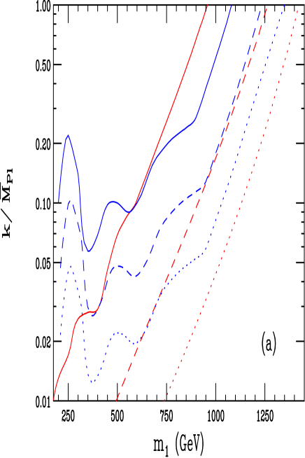
Figure 10: Exclusion region for resonance production of the first KK graviton excitation in the Drell-Yan (corresponding to the diagonal lines) and dijet (represented by the bumpy curves) channels at the Tevatron. The solid curves represent the results for Run I, while the dashed, dotted curves correspond to Run II with 2, 30 ${\rm fb}^{-1}$ of integrated luminosity, respectively. The excluded region lies above and to the left of the curves.

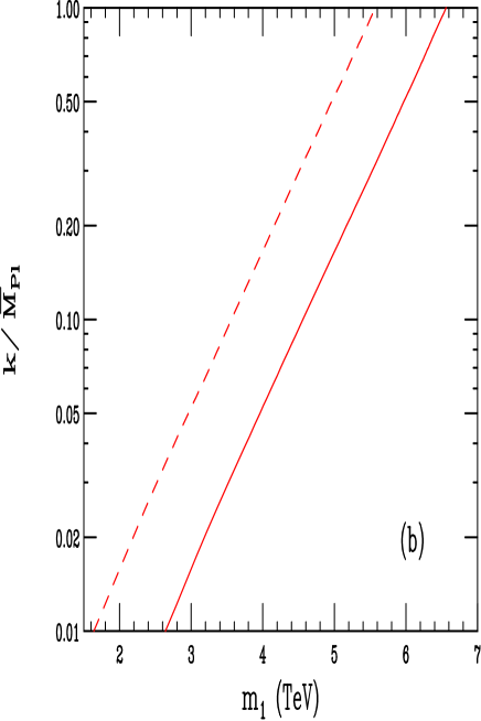
Figure 11: Exclusion region for resonance production of the first KK graviton excitation in the Drell-Yan production at the LHC. The dashed, solid curves correspond to 10, 100 ${\rm fb}^{-1}$ of integrated luminosity, respectively. The excluded region lies above and to the left of the curves.

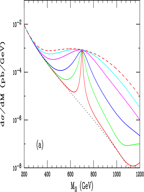
Figure 12: Drell-Yang production of the KK graviton with $M_{1}=700$ GeV at the Tevatron for $\eta=1,0.7,0.5,0.3,0.2$, and $0.1$, respectively, from top to bottom [72].

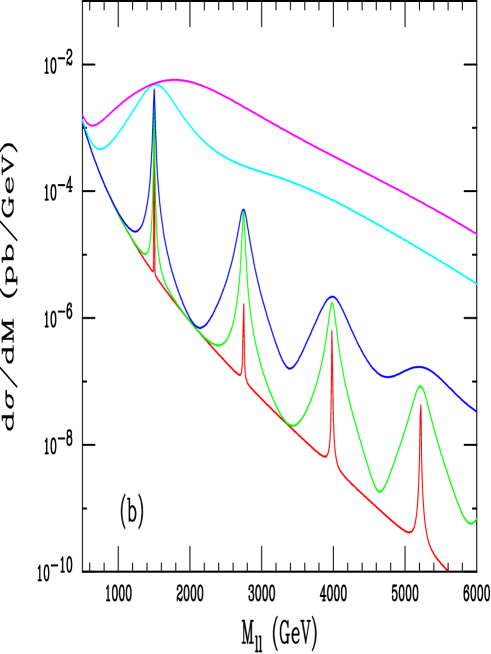
Figure 13: Drell-Yang production of the KK graviton with $M_{1}=1500$ GeV and its subsequent tower states at the LHC for $\eta=1,0.5,0.1,0.05,0.2$, and $0.01$, respectively, from top to bottom [72].

As an example let us discuss the possibility of detection of the resonance production of the first massive graviton in the proton - proton collisions $pp\rightarrow G^{(1)}\rightarrow e^{+}e^{-}$ at the LHC (ATLAS experiment) studied in Ref. [77]. The main background processes are $pp\rightarrow Z/\gamma^{*}\rightarrow e^{+}e^{-}$. By estimating the cross section of $G^{(1)}\rightarrow e^{+}e^{-}$ as a function of $M_{1}$ it was shown that the RS1 model would be detected if $M_{1}\leq 2080\;\mbox{GeV}$, see Fig. 14.

Figure 14: The cross-section times branching ratio, $\sigma\cdot B$, for $G^{(1)}\rightarrow e^{+}e^{-}$ in the RS1 model and the smallest detectable cross-section times the branching ratio, $(\sigma\cdot B)^{min}$ [77]. The plot is calculated for $\eta=0.01$.

To be able to conclude that the observed resonance is a graviton and not, for example, a spin-1 $Z^{\prime}$ or a similar particle it is necessary to check that it is produced by a spin-2 intermediate state. The spin of the intermediate state can be determined from the analysis of the angular distribution function $f(\theta)$ of the process, where $\theta$ is the angle between the initial and final beams. This function is $f=1$ for the scalar resonance, $f(\theta)=1+\cos^{2}\theta$ for a vector resonance, and is a polynomial of the 4th order in $\cos\theta$ for a spin-2 resonance. For example, for $gg\rightarrow G^{(1)}\rightarrow e^{+}e^{-}$ $f(\theta)=1-\cos^{4}\theta$, whereas for $q\bar{q}\rightarrow G^{(1)}\rightarrow e^{+}e^{-}$ $f(\theta)=1-3\cos^{2}\theta+4\cos^{4}\theta$. The analysis, carried out in Ref. [77], shows that angular distributions allow to determine the spin of the intermediate state with 90% C.L. for $M_{1}\leq 1720$ GeV.

As a next step it would be important to check the universality of the coupling of the first massive graviton $G^{(1)}$ by studing various processes, e.g. $pp\rightarrow G^{(1)}\rightarrow l^{+}l^{-},\;\mbox{jets},\;\gamma\gamma,W^{+}W^{-},HH$, etc. If it is kinematically feasible to produce higher KK modes, measuring the spacings of the spectrum will be another strong indication in favour of the RS1 model.

The conclusion drawn in Ref. [74] is that with the integrated luminocity ${\cal L}=100\;\mbox{fb}^{-1}$ the LHC will be able to cover the natural region of parameters $(M_{1},\eta)$ and, therefore, discover or exclude the RS1 model. This is illustrated in Fig. 15. The curves represent the theoretical constraint on the scalar curvature, Eq. (38) ($M_{5}=Me^{2k\pi R}$), the Tevatron bound (see Figs. 10, 11), the global fit from measurements of the oblique parameters S and T, and the bound $\Lambda_{\pi}<10\;\mbox{TeV}$. The latter is regarded as a condition for solving the hierarchy problem, i.e. it is supposed that if $\Lambda_{\pi}$ is large enough, namely $\Lambda_{\pi}\geq 10$TeV, the hierarchy remains and the motivation for introducing the RS1 model with one extra dimension is not sufficient. The range of the region in the $\eta$-direction is given by interval (40).

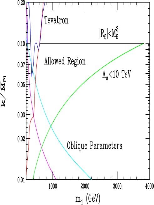
Figure 15: Summary of experimental and theoretical constraints on the parameters $M_{1}$ and $\eta=(k/M_{Pl})e^{k\pi R}$ of the RS1 model ($M_{1}$ is denoted as $m_{1}$ and $k/\bar{M}_{Pl}$ stands for $\eta$) [74]. The allowed region lies in the center as indicated.

There is an interesting phenomenology in theories when gauge fields and/or fermions of the SM are allowed to propagate in the bulk. We do not consider such cases here and present only a list of main references on the subject, see Refs. [36], [73], [74], [78] - [80].

In the present article we also do not analyze cosmological aspects of the RS models limiting ourselves only to a few short remarks. In a number of papers a Friedman-Robertson-Walker (FRW) generalization of the RS1 model was studied (see Refs. [64], [81], also Ref. [82] and an extensive list of references therein). Because of the presence of the branes the effective cosmological equations on the TeV-brane are non-standard. In particular, the effective Hubble parameter $H_{2}$ on this brane turns out to be proportional to the square of the energy density $\rho^{2}$ (and not to $\rho$, as in the standard cosmology), that for certain regimes leads to a contradiction with the standard behaviour of the scale factor of the three-dimensional space in the FRW Universe. In addition, the equation for $H_{2}$ includes an extra term which can be interpreted as an effective radiation term. However, as it was shown in Ref. [64], if a mechanism, stabilizing the radion (e.g. the Goldberger-Wise mechanism, Ref. [75]), is added, then the standard FRW cosmology is recovered for the temperatures $T<\Lambda_{\pi}$.

4 Discussion and Conclusions

We have considered two classes of models with extra dimensions, the ADD model and the RS-type models. The models were designed to solve the hierarchy problem. It turns out that they predict some new effects which can be detected at the existing (Tevatron) and future (LHC, TESLA) colliders. This opens new intriguing possibilities of discovering new physics and detecting extra dimensions of the space-time in high energy experiments in the near future. Their results may give us deeper understanding of the long standing hypothesis by T. Kaluza and O. Klein and even provide new arguments in favour or against it.

Limitations on the size of the article have not allowed us to include a number of interesting issues related to the ADD and RS models. In particular, we have not considered the neutrino physics within the KK approach. Apparently the idea of neutrinos experiencing extra dimensions was first introduced in articles [83], and later was developed in Refs. [79], [84]. Also topics like the analysis of the anomalous magnetic moment of the muon (see Ref. [85]), latest developments in SUSY extensions of the SM with extra dimensions (see Refs. [35], [38]), latest results on astrophysics with extra dimensions (see, for example, Ref. [86] and references therein), and many others are left beyond the scope of the present review.

We finish the article with a short summary of main features of the ADD and RS models.

ADD Model.

1. The ADD model removes the $M_{EW}/M_{Pl}$ hierarchy, but replaces it by the hierarchy

   $$\frac{R^{-1}}{M}\sim\left(\frac{M}{M_{Pl}}\right)^{2/d}\sim 10^{-\frac{30}{d}}.$$

   For $d=2$ this relation gives $R^{-1}/M\sim 10^{-15}$. This hierarchy is of different type and might be easier to understand or explain, perhaps with no need for SUSY.

2. The scheme is viable.

3. For $M$ small enough high energy physics effects, predicted by the model, can be discovered at future collider experiments.

4. For $d=2$ the cosmological and astrophysical bounds on $M$ are high enough ($M\geq 100$ TeV), so that a (mild) hierarchy is already re-introduced. For $d\geq 3$ the bounds on $M$ are sufficiently low.

5. Some natural cosmological scenarios within the ADD approach may bring further problems. One of them is the $m_{inf}/M$ hierarchy, where $m_{inf}$ is the mass of the inflaton (see Eq. (28)). Another is the moduli problem. These may be indications of the need for SUSY in multidimensional theories.

RS1 model

1. The model solves the $M_{EW}/M_{Pl}$ hierarchy problem without generating a new hierarchy.

2. A large part of the allowed range of parameters of the RS1 model will be studied in future collider experiments which will either discover the RS1 model or exclude the most ”natural” region of its parameter space (see Sect. 3.2).

3. With a mechanism of radion stabilization added the model is quite viable. In this case cosmological scenarios, based on the RS1 model, are consistent without additional fine-tuning of parameters (except the cosmological constant problem).

References

- [1] T. Kaluza, Sitzungsber. Preuss. Akad. Wiss., Phys.-Math.Kl., Berlin Math. Phys., Bd. K1 (1921) 966.
- [2] O. Klein, Z. Phys. 37 (1926) 895.
-
[3]
A. Salam and J. Strathdee, Ann. Phys. 141 (1982) 316.
W. Mecklenberg, Fortschr. d. Phys. 32 (1984) 207.
I.Ya. Arefeva, I.V. Volovich, Sov. Phys. Usp. 28 (1985) 694; Usp. Fiz. Nauk 146 (1985) 655.
M.J. Duff, B.E.W. Nilsson and C.N. Pope, Phys. Rep. 130C (1986) 1.
T. Appelquist, A. Chodos and P.G.O. Freund, ”Modern Kaluza-Klein Theories”. Reading, MA, Addison-Wesley, 1987. - [4] Yu.A. Kubyshin, J.M. Mourão, G. Rudolph and I.P. Volobuev, ”Dimensional Reduction of Gauge Theories, Spontaneous Compactification and Model Building”. Lecture Notes in Physics, v. 349. Berlin, Springer-Verlag, 1989.
- [5] D.Kapetanakis and G.Zoupanos, Phys. Rept. C219 (1992) 1.
- [6] N. Arkani-Hamed, S. Dimopoulos and G. Dvali, Phys. Lett. B429 (1998) 263 [hep-ph/9803315].
- [7] N. Arkani-Hamed, S. Dimopoulos and G. Dvali, Phys.Rev. D59 (1999) 086004 [hep-ph/9807344].
- [8] L. Randall and R. Sundrum, Phys. Rev. Lett. 83 (1999) 3370 [hep-ph/9905221].
- [9] L. Randall and R. Sundrum, Phys. Rev. Lett. 83 (1999) 4690 [hep-th/9906064].
- [10] I. Antoniadis, ”String and D-brane Physics at Low Energy”, hep-th/0102202.
- [11] R.-D. Heuer, D.J. Miller, F. Richard and P.M. Zerwas (editors), ”TESLA. Technical Design Report. Part III: Physics at an Linear Collider.” DESY 2001-011 (March 2001), hep-ph/0106315.
- [12] V.A. Rubakov, ”Large and infinite extra dimensions”, hep-ph/0104152.
- [13] M. Besançon, ”Experimental introduction to extra dimensions”, hep-ph/0106165.
-
[14]
E. Witten, Phys. Rev. Lett. 38 (1977) 121.
N.S. Manton, Nucl. Phys. B158 (1979) 141.
P. Forgacs and N.S. Manton, Comm. Math. Phys. 72 (1980) 15. - [15] P. Manousselis and G. Zoupanos, Phys. Lett. B504 (2001) 122 [hep-ph/0010141]; Phys. Lett. B518 (2001) 171 [hep-ph/0106033]; ”Dimensional Reduction over Coset Spaces and Supersymmetry Breaking”, hep-ph/0111125.
-
[16]
A. Datta, P.J. O’Donnell, Z.-H. Lin, X. Zhang, T. Huang,
Phys. Lett. B483 (2000) 203 [hep-ph/0001059].
D. Bourilkov, ”Two-fermion and Two-photon Final States at LEP2 and Search for Extra Dimensions”, hep-ex/0103039.
T. Appelquist, Hsin-Chia Cheng and B.A. Dobrescu, Phys. Rev. D64 (2001) 035002 [hep-ph/0012100].
A. Mück, A. Pilaftsis and R. Rückl, ”Minimal Higher-Dimensional Extensions of the Standard Model and Electroweak Observable”, hep-ph/0110391. - [17] V. Rubakov and M. Shaposhnikov, Phys. Rev. B125 (1983) 136.
- [18] K. Akama, Lect. Notes Phys. 176 (1982) 267 [hep-th/0001113].
- [19] G. Dvali and M. Shifman, Phys. Lett. B396 (1997) 64.
- [20] I. Antoniadis, N. Arkani-Hamed, S. Dimopoulos and G. Dvali, Phys.Lett. B436 (1998) 257 [hep-ph/9804398].
- [21] J. Polchinski, ”TASI lectures on D-branes”, hep-th/9611050.
- [22] C.P. Bachas, ”Lectures on D-branes”, hep-th/9806199.
-
[23]
P. Hořava and E. Witten, Nucl. Phys. B460 (1996) 506.
- [24] P. Hořava and E. Witten, Nucl. Phys. B475 (1996) 94.
- [25] E. Witten, Nucl. Phys. B471 (1996) 135.
- [26] T. Banks and M. Dine, Nucl. Phys. B479 (1996) 173.
- [27] A. Lukas, B.A. Ovrut, K.S. Stelle, and D. Waldram, Phys. Rev. D59 (1999) 086001 [hep-th/9803235].
- [28] K.R. Dienes, E. Dudas and T. Gherghetta, Nucl.Phys. B537 (1999) 47 [hep-ph/9806292].
- [29] R. Sundrum, Phys. Rev. D59 (1999) 085010 [hep-ph/9807348].
- [30] L. Anchordoqui, Carlos Nuñez and Kasper Olsen, JHEP 0010 (2000) 050 [hep-th/0007064].
- [31] J. Lykken, Phys. Rev. D54 (1996) 3693.
- [32] K.R. Dienes, E. Dudas and T. Gherghetta, Phys. Lett. B436 (1998) 55 [hep-ph/9803466].
-
[33]
S. Dimopoulos and H. Georgi, Nucl. Phys. B193 (1981) 150.
P. Hořava, Phys. Rev. D54 (1996) 7561.
E. Mirabelli and M. Peskin, Phys. Rev. D58 (1998) 065002.
H. Nilles, M. Olechowski and M. Yamaguchi, Nucl.Phys. B530 (1998) 43. - [34] J. Scherk and J.H. Schwarz, Phys. Lett. B82 (1979) 60; Nucl.Phys. B153 (1979) 61.
- [35] A. Pomarol and M. Quirós, Phys. Lett. B438 (1998) 255 [hep-ph/9806263].
- [36] T. Gherghetta and A. Pomarol, Nucl. Phys. B586 (2000) 141 [hep-ph/0003129].
- [37] T. Gherghetta and A. Pomarol, Nucl. Phys. B602 (2001) 3 [hep-ph/0012378].
-
[38]
A. Delgado, A. Pomarol and M. Quirós, Phys. Rev. D60
(1999) 095008 [hep-ph/9812489].
R. Barbieri, L.J. Hall and Y. Nomura, Phys. Rev. D63 (2001) 105007 [hep-ph/0011311]. - [39] D.E. Kaplan and T.M.P. Tait, JHEP 0006 (2000) 020 [hep-ph/0004200]; ”New Tools for Fermion Masses from Extra Dimensions”, hep-ph/0110126.
- [40] T. Kobayashi, J. Kubo, M. Mondragon and G. Zoupanos, Nucl. Phys. B550 (1999) 99 [hep-ph/9812221].
-
[41]
Yu.A. Kubyshin, D. O’Connor and C.R. Stephens, Class. Quant.
Grav. 10 (1993) 2519.
J.Kubo, H.Terao and G.Zoupanos, Nucl. Phys. B574 (2000) 495 [hep-ph/9910277]. - [42] I. Antoniadis, Phys. Lett. B246 (1990) 377.
-
[43]
I. Antoniadis, C. Muñoz and M. Quirós, Nucl.Phys. B397
(1993) 515 [hep-ph/9211309].
I. Antoniadis and K. Benakli, Phys. Lett. B326 (1994) 69 [hep-ph/9310151].
I. Antoniadis, K. Benakli and M. Quirós, Phys. Lett. B331 (1994) 313 [hep-ph/9403290]. - [44] A. Demichev, Yu. Kubyshin and J.I. Pérez-Cadenas, Phys. Lett. B323 (1994) 139 [hep-th/9310093].
- [45] C.D. Hoyle et al., Phys. Rev. Lett. 86 (2001) 1418 [hep-ph/0011014].
- [46] G.F. Giudice, R. Rattazzi and J.D. Wells, Nucl. Phys. B544 (1999) 3 [hep-ph/9811291].
- [47] T. Han, J.D. Lykken and Ren-Jie Zhang, Phys. Rev. D59 (1999) 105006 [hep-ph/9811350].
- [48] E.A. Mirabelli, M. Perelstein and M.E. Peskin, Phys. Rev. Lett. 82 (1999) 2236 [hep-ph/9811337].
- [49] J.L. Hewett, Phys. Rev. Lett. 82 (1999) 4765 [hep-ph/9811356].
- [50] T.G. Rizzo, Phys. Rev. D59 (1999) 115010 [hep-ph/9901209].
- [51] K. Cheung, W.-Y. Keung, Phys. Rev. D60 (1999) 112003 [hep-ph/9903294].
- [52] G. Wilson, LC-PHSM-2001-010.
- [53] L. Vacavant and I. Hinchliffe, ”Model Independent Extra-dimension signatures with ATLAS”, hep-ex/0005033.
- [54] S. Hannestad, Phys. Rev. D64 (2001) 023515 [hep-ph/0102290].
- [55] S. Cullen and M. Perelstein, Phys. Rev. Lett. 83 (1999) 268 [hep-ph/9903422].
-
[56]
C. Hanhart, D.R. Phillips, S. Reddy and M.J. Savage,
Nucl. Phys. B595 (2001) 335-359 [nucl-th/0007016].
C. Hanhart, J.A. Pons, D.R. Phillips and S. Reddy, Phys. Lett. B509 (2001) 1 [astro-ph/0102063].
M. Fairbairn, Phys. Lett. B508 (2001) 335 [hep-ph/0101131].
V. Barger, T. Han, C. Kao and R.-J. Zhang, Phys. Lett. B461 (1999) 34 [hep-ph/9905474]. - [57] L.J. Hall and D. Smith, Phys. Rev. D60 (1999) 085008 [hep-ph/9904267].
- [58] S.C. Kappadath et al., BAAS 30 (2) (1998) 926.
- [59] S. Hannestad and G.G. Raffelt, Phys. Rev. Lett. 87 (2001) 051301 [hep-ph/0103201].
- [60] N. Kaloper and A. Linde, Phys. Rev. D59 (1999) 101303 [hep-th/9811141].
- [61] D. Lyth, Phys. Lett. B448 (1999) 191 [hep-ph/9810320].
- [62] R.N. Mohapatra, A. Pérez-Lorenzana and C. de S. Pires, Phys. Rev. D62 (2000) 105030 [hep-ph/0003089].
- [63] N. Arkani-Hamed, S. Dimopoulos and J. March-Russel, Phys. Rev. D63 (2001) 064020 [hep-th/9809124].
- [64] C. Csáki, M.L. Graesser, L. Randall and J. Terning, Phys. Rev. D62 (2000) 045015 [hep-ph/9911406].
- [65] W.D. Goldberger and M.B. Wise, Phys. Lett. B475 (2000) 275 [hep-ph/9911457].
- [66] C. Charmousis, R. Gregory and V. Rubakov, Phys. Rev. D62 (2000) 067505 [hep-th/9912160].
- [67] L. Pilo, R. Rattazzi and A. Zaffaroni, JHEP 0007 (2000) 056 [hep-th/0004028].
- [68] I.Ya. Aref’eva, M.G. Ivanov, W. Mueck, K.S. Viswanathan and I.V. Volovich, Nucl. Phys. B590 (2000) 273 [hep-th/0004114].
- [69] E.E. Boos, Yu.A. Kubyshin, M.N. Smolyakov and I.P. Volobuev, ”Effective Lagrangians for linearized gravity in Randall-Sundrum model”, hep-th/0105304.
- [70] B. Grinstein, D.R. Nolte and W. Skiba, Phys. Rev. D63 (2001) 105005 [hep-th/0012074].
- [71] J. Lykken and L. Randall, JHEP 0006 (2000) 014 [hep-th/9908076].
- [72] H. Davoudiasl, J.H. Hewett and T.G. Rizzo, Phys. Rev. Lett. 84 (2000) 2080 [hep-ph/9909255].
- [73] H. Davoudiasl, J.H. Hewett and T.G. Rizzo, Phys. Lett. B473 (2000) 43 [hep-ph/9911262].
- [74] H. Davoudiasl, J.H. Hewett and T.G. Rizzo, Phys. Rev. D63 (2001) 075004 [hep-ph/0006041].
- [75] W.D. Goldberger and M.B. Wise, Phys. Rev. Lett. 83 (1999) 4922 [hep-ph/9907447].
-
[76]
G.F. Giudice, R. Rattazzi and J.D. Wells, Nucl. Phys. B595
(2001) 250 [hep-ph/0002178].
C. Csáki, M.L. Graesser and G.D. Kribs, Phys. Rev. D63 (2001) 016002 [hep-th/0008151].
T. Han, G.D. Kribs and B. McElrath, Phys. Rev. D64 (2001) 076003 [hep-ph/0104074]. - [77] B.C. Allanach, K. Odagiri, M.A. Parker and B.R. Webber, JHEP 0009 (2000) 019 [hep-ph/0006114].
-
[78]
A. Pomarol, Phys. Lett. B486 (2000) 153 [hep-ph/9911294].
S. Chang, J. Hisano, H. Nakano, N. Okada and M. Yamaguchi, Phys. Rev. D62 (2000) 084025 [hep-ph/9912498].
B. Bajc and G. Gabadadze, Phys. Lett. B474 (2000) 282 [hep-th/9912232]. - [79] Y. Grossman and M. Neubert, Phys. Lett. B474 (2000) 361 [hep-ph/9912408].
- [80] S.J. Huber and Q. Shafi, Phys. Rev. D63 (2001) 045010 [hep-ph/0005286]; Phys. Rev. D63 (2001) 045010 [hep-ph/0005286]; Phys. Rev. D63 (2001) 045010 [hep-ph/0005286].
-
[81]
C. Csáki, M.L. Graesser and J. Terning, Phys.Lett.
B456 (1999) 16 [hep-ph/9903319].
P. Binétruy, C. Deffayet and D. Langlois, Nucl. Phys. B565 (2000) 269 [hep-th/9905012].
C. Csáki, M.L. Graesser, C. Kolda and J. Terning, Phys. Lett. B462 (1999) 34 [hep-ph/9906513].
J.M. Cline, C. Grojean and G. Servant, Phys. Rev. Lett. 83 (1999) 4245 [hep-ph/9906523].
T. Shiromizu, K. Maeda and M. Sasaki, ”The Einstein Equations on the 3-Brane World”, Phys. Rev. D62 (2000) 024012 [gr-qc/9910076].
P. Binétruy, C. Deffayet, U. Ellwanger and D. Langlois, Phys. Lett. B477 (2000) 285 [hep-th/9910219].
S. Tsujikawa, K. Maeda and S. Mizuno, Phys. Rev. D63 (2001) 123511 [hep-ph/0012141].
P. Binétruy, C. Deffayet and D. Langlois, ”The radion in brane cosmology”, hep-th/0101234. - [82] L. Anchordoqui, J. Edelstein, C. Nuñez, S. Perez Bergliaffa, M. Schvellinger, M. Trobo and F. Zyserman, Phys. Rev. D64 (2001) 084027 [hep-th/0106127].
-
[83]
K.R. Dienes, E. Dudas and T. Gherghetta, Nucl. Phys.
B557 (1999) 25 [hep-ph/9811428].
N. Arkani-Hamed, S. Dimopoulos, G. Dvali and J. March-Russell, ”Netrino Masses from Large Extra Dimensions”, hep-ph/9811448. -
[84]
A. Lukas, P. Ramond, A. Romanino and G.G. Ross, JHEP 0104
(2001) 010 [hep-ph/0011295].
J. Maalampi, V.Sipiläinen and I. Vilja, Phys. Lett. B512 (2001) 91 [hep-ph/0103312].
D. Monderen, ”Solar and atmospheric neutrinos: a solution with large extra dimensions”, hep-ph/0104113.
A. Gouvea, G. Giudice, A. Strumia and K. Tobe, ”Phenomenological implications of neutrinos in extra dimensions”, hep-ph/0107156. -
[85]
H. Davoudiasl, J.H. Hewett and T.G. Rizzo, Phys. Lett. B493 (2000)
135 [hep-ph/0006097].
S.C.Park and H.S.Song, Phys. Lett. B506 (2001) 99 [hep-ph/0103072].
C.S. Kim, J.D. Kim and J. Song, Phys.Lett. B511 (2001) 251 [hep-ph/0103127].
K. Agashe, N.G. Deshpande, G.-H. Wu, Phys. Lett. B511 (2001) 85 [hep-ph/0103235]. - [86] K.A. Postnov, ”Gamma-Ray Bursts: Super-Explosions in the Universe and Related High-Energy Phenomena”, see these Proceedings [astro-ph/0107122].