$\gamma^{*}\gamma^{(*)}\to\pi$ transitions and the pion distribution amplitude

Abstract:

We discuss what can be learned about the shape of the pion distribution amplitude from the form factor for $\gamma^{*}\gamma^{(*)}\to\pi$ transitions.

1 Introduction

The determination of hadronic distribution amplitudes by theoretical as well as by experimental means has been and still is an active area of research. The form factor $F_{\pi\gamma}$ for transitions $\gamma^{*}\gamma\to\pi$, for instance, has been discussed by many authors in order to find constraints for the shape of the pion distribution amplitude [1, 2, 3], to name but a few. The pion distribution amplitude is an important ingredient in, e.g., the electromagnetic pion form factor, pion pair production in two-photon collisions and, moreover, in exclusive B meson decays into pseudo-scalars, where strong interaction effects are currently under active investigation.

In this talk we discuss the transition form factor $F_{\pi\gamma^{*}}$ for doubly virtual photons [4], $\gamma^{*}\gamma^{*}\to\pi$, and explore what can be learned from it beyond what is already known from the case of the real-photon limit $\gamma^{*}\gamma\to\pi$.

2 The transition form factor $F_{\pi\gamma^{*}}$

We consider the case of space-like photon virtualities, denoted by $Q^{2}=-q^{2},\,Q^{\prime 2}=-q^{\prime 2}$, which is accessible in $e^{+}e^{-}\to e^{+}e^{-}\pi$. It is convenient to define $\overline{Q}\hskip 1.0pt^{2}=(Q^{2}+Q^{\prime 2})/2,\,\omega=(Q^{2}-Q^{\prime 2})/(Q^{2}+Q^{\prime 2})$. When at least one of the two photon virtualities is large compared to a hadronic scale the $\gamma^{*}\gamma^{*}\to\pi$ form factor factorises into a partonic hard scattering amplitude and a soft hadronic matrix element, which is parametrised by the universal pion distribution amplitude $\Phi_{\pi}$ [5]. The leading twist, next-to-leading order (NLO) $\alpha_{s}$ expression for $F_{\pi\gamma^{*}}$ is given by [6, 7]:

$$F_{\pi\gamma^{*}}(\overline{Q},\omega)=\frac{f_{\pi}}{3\sqrt{2}\,\overline{Q}\hskip 1.0pt^{2}}\,\int_{-1}^{\;1}{d}\xi\,\frac{\Phi_{\pi}(\xi,\mu_{F})}{1-\xi^{2}\omega^{2}}\,\left[1+\frac{\alpha_{s}(\mu_{R})}{\pi}\,{\cal K}(\omega,\xi,\overline{Q}/\mu_{F})\right]\,,$$ (1)

The function ${\cal K}(\omega,\xi,\overline{Q}/\mu_{F})$ is the NLO hard scattering kernel in the $\overline{\rm MS}$ scheme. $\Phi_{\pi}(\xi,\mu_{F})$ is the distribution amplitude of the pion’s valence Fock state with $\xi=2x-1$ and $x$ being the light-cone momentum fraction of the quark. $\mu_{F}$ is the factorisation scale and $\mu_{R}$ denotes the renormalisation scale, both of which are to be taken of order $\overline{Q}$. $f_{\pi}\approx 131\,{\rm MeV}$ is the pion decay constant. The pion distribution amplitude can be expanded in terms of the Gegenbauer polynomials $C_{n}^{3/2}(\xi)$, the eigenfunctions of the leading-order (LO) evolution kernel [5]:

$$\Phi_{\pi}(\xi,\mu_{F})=\Phi_{\rm AS}(\xi)\left[1+\sum^{\infty}_{n=2,4,...}B_{n}(\mu_{F})\,C_{n}^{3/2}(\xi)\right]\,.$$ (2)

To lowest order, the scale dependent Gegenbauer coefficients $B_{n}$ are known to evolve according to

$$B_{n}(\mu_{F})=B_{n}(\mu_{0})\,\left(\frac{\alpha_{s}(\mu_{F})}{\alpha_{s}(\mu_{0})}\right)^{\gamma_{n}/\beta_{0}}\,,$$ (3)

where $\mu_{0}$ is a reference scale which we choose to be 1 GeV and $\beta_{0}=11-2n_{f}/3$. The anomalous dimensions $\gamma_{n}$ are positive numbers increasing with $n$ such that for large scales any distribution amplitude evolves into the asymptotic form, given by

$$\Phi_{\rm AS}(\xi)=\frac{3}{2}(1-\xi^{2})\,.$$ (4)

It immediately follows that in the real-photon case (i.e., $\omega=\pm 1$) the transition form factor approaches the limit

$$F_{\pi\gamma}(\overline{Q},\omega=\pm 1)\longrightarrow\frac{f_{\pi}}{\sqrt{2}\,\overline{Q}\hskip 1.0pt^{2}}$$ (5)

as $\ln\mu_{F}$ becomes large. Note that this is a parameter-free QCD prediction, given that $f_{\pi}$ is known.

Using the Gegenbauer expansion (2) the form factor (1) can be written as

$$F_{\pi\gamma^{*}}(\overline{Q},\omega)=\frac{f_{\pi}}{\sqrt{2}\>\overline{Q}\hskip 1.0pt^{2}}\left[c_{0}(\omega,\mu_{R})+\sum_{n=2,4,\ldots}c_{n}(\omega,\mu_{R},\overline{Q}/\mu_{F})\,B_{n}(\mu_{F})\right]\,,$$ (6)

with analytically computable functions $c_{n}$, which characterise the sensitivity of $F_{\pi\gamma^{*}}$ to the Gegenbauer coefficients $B_{n}$. The lowest coefficients $c_{n}$ are shown in Fig. 1. Here and in the following we use the two-loop expression of $\alpha_{s}$ with $n_{f}=4$, $\Lambda^{(4)}_{\overline{\rm MS}}=305\,{\rm MeV}$ and we set $\mu_{F}=\mu_{R}=\overline{Q}$. We see that for $n\geq 2$ the functions $c_{n}$ show a very fast decrease as $\omega\to 0$, i.e., the transition form factor is sensitive to the coefficients $B_{n}$ only in the real-photon limit $\omega\to 1$. At $\omega=1$ we find

$$c_{n}(\omega=1)=1+\frac{\alpha_{s}(\mu_{R})}{\pi}\,{\cal K}_{n}(\omega=1,\overline{Q}/\mu_{F})\,,$$ (7)

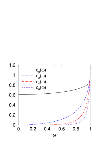
Figure 1: The coefficients $c_{n}(\omega)$ in the expansion (6) of the $\gamma^{*}$–$\,\pi$ transition form factor. NLO corrections are included with $\mu_{F}=\mu_{R}=\overline{Q}$, which is taken as 2 GeV.

which implies that the $\gamma$–$\pi$ transition form factor approximately probes the sum $1+\sum_{n}B_{n}$ of Gegenbauer coefficients. In order to extract information about individual Gegenbauer coefficients from the experimental data [8] on the form factor one therefore has to truncate the Gegenbauer series at some $n_{0}$ and assume $B_{n}=0$ for $n\geq n_{0}$. Taking $n_{0}=4$, for example, we find $B_{2}(\mu_{0}=1\,{\rm GeV})=-0.06\pm 0.03$. Here we have restricted the experimentally available range of $Q^{2}$ to some $Q^{2}_{\rm min}$ between 2 and 3 GeV², which is necessary to exclude large contributions from next-to-leading twist corrections. Further sources of uncertainty result from the experimental errors and from the fact that the choice of $\mu_{F}$ and $\mu_{R}$ is not unique at finite order of perturbation theory.

Allowing for nonzero $B_{2}$ and $B_{4}$ it is not possible to find unique values for these coefficients since there is a linear correlation between $B_{2}$ and $B_{4}$, which is only slightly resolved due to a mild logarithmic dependence and due to experimental errors. Performing a fit to the data with $Q^{2}_{\rm min}=2\,{\rm GeV}^{2}$ we find $B_{2}+B_{4}=-0.06\pm 0.08$ and $B_{2}-B_{4}=0.0\pm 0.9$ at $\mu_{0}=1\,{\rm GeV}$. Thus, it might well be that the individual Gegenbauer coefficients are small and the pion distribution amplitude is close to its asymptotic form. On the other hand, with the presently available data on the $\gamma$–$\pi$ transition form factor, we cannot exclude large Gegenbauer coefficients the sum of which being close to zero due to cancellations.

Apart from the above mentioned uncertainties, there are also power corrections which could spoil the phenomenological analysis and which we would like to briefly comment on. For $\omega$ close to 1, the convolution (1) is sensitive to the endpoint regions $\xi\to\pm 1$. This corresponds to the situation in which one of the quarks in the pion has small momentum fraction such that soft effects become important. In particular, corrections arising from partonic transverse momenta are non-negligible. In order to estimate these corrections, we follow the modified perturbative approach of Refs. [9, 10]. Here, the expression (1) is replaced by a convolution of Fourier transforms of the pion light-cone wave function, the modified hard scattering kernel at LO $\alpha_{s}$ and the Sudakov factor, which accounts for resummed gluonic radiative corrections which are not contained in the wave function:

$$F_{\pi\gamma^{*}}(\overline{Q},\omega)=\frac{1}{4\sqrt{3}\pi^{2}}\int{d}\xi\,{d}^{2}{\bf b}\,\hat{\Psi}_{\pi}^{*}(\xi,-{\bf b},\mu_{F})\,K_{0}(\sqrt{1+\xi\omega}\>\overline{Q}\,b)\,\exp\left[-S\left(\xi,b,\overline{Q},\mu_{R}\right)\right]\,.$$ (8)

Since the transverse separation $b$ acts as an infrared cut-off, the factorisation scale $\mu_{F}$ is set equal to $1/b$. As the renormalisation scale $\mu_{R}$ we take the largest mass scale occuring in the propagator of the internal quark, $\mu_{R}=\max{\{1/b,\sqrt{1+\xi\omega}\>\,\overline{Q},\sqrt{1-\xi\omega}\>\,\overline{Q}\}}$ [10]. Following [11, 12] we assume for the light-cone wave function in $b$-space the simple form

$$\hat{\Psi}_{\pi}(\xi,{\bf b})=\frac{2\pi f_{\pi}}{\sqrt{6}}\,\Phi_{\rm AS}(\xi)\exp{\left[-\frac{\pi^{2}f_{\pi}^{2}}{2}(1-\xi^{2})\,b^{2}\right]}$$ (9)

in our estimate. The prediction of the $\gamma$–$\pi$ transition form factor in the modified perturbative approach using this wave function leads to very good agreement with the CLEO data [13].

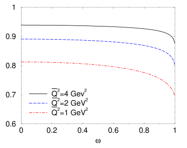
Figure 2: Ratio of $F_{\pi\gamma^{*}}(\overline{Q},\omega)$ in the modified perturbative approach and in the LO leading-twist approximation at $\overline{Q}\hskip 1.0pt^{2}=4\,{\rm GeV}^{2}$ (solid line), $\overline{Q}\hskip 1.0pt^{2}=2\,{\rm GeV}^{2}$ (dashed line), and $\overline{Q}\hskip 1.0pt^{2}=1\,{\rm GeV}^{2}$ (dash-dotted line). Here we have used the wave function (9) in the modified perturbative approach and the asymptotic pion distribution amplitude.

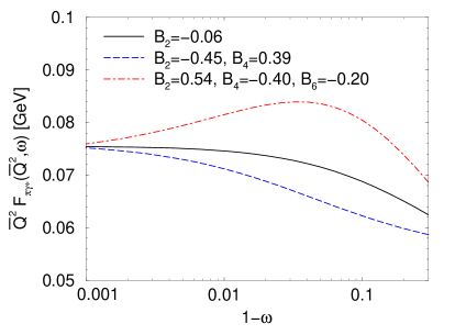
Figure 3: The scaled form factor $\overline{Q}\hskip 1.0pt^{2}F_{\pi\gamma^{*}}(\overline{Q},\omega)$ calculated to NLO in the leading-twist approximation at $\overline{Q}^{2}=4\,{\rm GeV}^{2}$, using sample distribution amplitudes. The values of the Gegenbauer coefficients are quoted at the scale $\mu_{0}=1\,{\rm GeV}$. All higher order Gegenbauer coefficients are taken to be zero.

In Fig. 3 we show the ratio of the predictions of the form factor in the modified perturbative approach and in leading-twist approximation at LO in $\alpha_{s}$. In both approximations we employ the asymptotic form of the pion distribution amplitude. We see that the power corrections are less than about 10% for $\overline{Q}^{2}=4\,{\rm GeV}^{2}$. Note that the Sudakov corrections amount to no more than 1.5% such that it is sufficient to retain only the leading logarithmic terms in the Sudakov function $S$ as given in Ref. [9].

We have also checked that the results of Fig. 3 essentially remain unchanged for $\omega\raisebox{-4.0pt}{$\,\stackrel{{\scriptstyle\textstyle<}}{{\sim}}\,$}0.8$ when we include an effective mass $m_{\rm eff}=0.33\,{\rm GeV}$ in the light-cone wave function (9) with appropriately adjusted parameters, as proposed in Ref. [11], for example. For $\omega\raisebox{-4.0pt}{$\,\stackrel{{\scriptstyle\textstyle>}}{{\sim}}\,$}0.8$ the ratio then becomes up to 10% smaller, since the inclusion of the mass term leads to a stronger suppression of the endpoint regions in the modified perturbative approach.

Although Fig. 1 clearly shows that in practice one cannot gain new informations on the Gegenbauer coefficients from $\gamma^{*}\gamma^{*}\to\pi$ transitions in a wide range of $\omega$, one can nevertheless use the region where $\omega$ is close to but different from 1 to obtain valuable informations beyond what is already known from the real-photon limit. This is demonstrated in Fig. 3, where we plot the form factor for different choices of distribution amplitudes. The kinematical range shown allows for a discrimination between distribution amplitudes with small individual Gegenbauer coefficients and distribution amplitudes with large $B_{n}$ the sum of which being small in compliance with the constraint from the real-photon limit.

We now turn to the kinematical region where $\omega$ significantly differs from 1. The fast decrease of the functions $c_{n}$ can be understood by expanding the hard scattering kernel in Eq. (1) for small $\omega$. Remarkably, one finds that each coefficient $B_{n}$ is suppressed by a corresponding factor $\omega^{n}$. Neglecting terms of ${\cal O}(\omega^{4})$ we obtain

$$F_{\pi\gamma^{*}}(\overline{Q},\omega) = \frac{\sqrt{2}f_{\pi}}{3\>\overline{Q}\hskip 1.0pt^{2}}\left[1-\frac{\alpha_{s}}{\pi}+\frac{1}{5}\,\omega^{2}\left(1-\frac{5}{3}\frac{\alpha_{s}}{\pi}\right)\phantom{\frac{\overline{Q}\hskip 1.0pt^{2}}{\mu_{F}^{2}}}\right.$$ (10)

$$\hskip 20.00003pt\left.{}+\frac{12}{35}\,\omega^{2}B_{2}(\mu_{F})\left(1+\frac{5}{12}\frac{\alpha_{s}}{\pi}\left\{1-\frac{10}{3}\ln\frac{\overline{Q}\hskip 1.0pt^{2}}{\mu_{F}^{2}}\right\}\right)\right]+{\cal O}(\omega^{4},\alpha_{s}^{2}).\;\;$$

For $\omega\to 0$ we thus have a parameter-free prediction from QCD to leading-twist accuracy, which is even valid over a wide range of $\omega$:

$$F_{\pi\gamma^{*}}(\overline{Q},\omega)=\frac{\sqrt{2}f_{\pi}}{3\>\overline{Q}\hskip 1.0pt^{2}}\bigg{[}1-\frac{\alpha_{s}}{\pi}\bigg{]}+{\cal O}(\omega^{2},\alpha_{s}^{2})\,.$$ (11)

To LO $\alpha_{s}$, this result is known since long, see Ref. [14]. The $\alpha_{s}$-correction to the leading term can be found in Ref. [6]. Any observed deviation from the leading-twist prediction would be a signal for large power corrections and therefore, this prediction well deserves experimental verification. For small $\omega$, the relation (11) has a status comparable to the famous expression of the cross section ratio $R=\sigma(e^{+}e^{-}\to{\rm hadrons})/\sigma(e^{+}e^{-}\to\mu^{+}\mu^{-})$.

References

- [1] R. Jakob, P. Kroll and M. Raulfs, J. Phys. G 22 (1996) 45.
- [2] I.V. Musatov and A.V. Radyushkin, Phys. Rev. D 56 (1997) 2713.
- [3] S.J. Brodsky, C.-R. Ji, A. Pang and D.G. Robertson, Phys. Rev. D 57 (1998) 245.
- [4] M. Diehl, P. Kroll and C. Vogt, Eur. Phys. J. C, in press [hep-ph/0108220].
- [5] G.P. Lepage and S.J. Brodsky, Phys. Rev. D 22 (1980) 2157.
- [6] F. Del Aguila and M.K. Chase, Nucl. Phys. B 193 (1981) 517.
- [7] E. Braaten, Phys. Rev. D 28 (1983) 524.
- [8] J. Gronberg et al., CLEO collaboration, Phys. Rev. D 57 (1998) 33.
- [9] J. Botts and G. Sterman, Nucl. Phys. B 325 (1989) 62.
- [10] H.-N. Li and G. Sterman, Nucl. Phys. B 381 (1992) 129.
- [11] S. J. Brodsky, T. Huang and G. P. Lepage, Particles and Fields, Vol. 2, edited by A. Z. Capri and A. N. Kamal, Banff Summer Institute, 1981, (Plenum, New York, 1983), p. 143.
- [12] R. Jakob and P. Kroll, Phys. Lett. B 315 (1993) 463.
- [13] P. Kroll and M. Raulfs, Phys. Lett. B 387 (1996) 848.
-
[14]
J.M. Cornwall,
Phys. Rev. D 16 (1966) 1174;
G. Köpp, T.F. Walsh and P. Zerwas, Nucl. Phys. B 70 (1974) 461.