CP violating neutrino oscillation
and uncertainties in Earth matter density

Abstract

We propose a statistical formulation to estimate possible errors in long baseline neutrino oscillation experiments caused by uncertainties in the Earth matter density. A quantitative investigation of the effect is made on the CP asymmetry in future neutrino factory experiments.

Leptonic CP violation (CPV) is one of the main challenges in future long baseline (LBL) neutrino oscillation experiments [1], where more accurate measurements of the neutrino oscillation parameters are anticipated. However, since the neutrino beam travels a long path through the Earth, the MSW matter effect [2] can mimic a non-vanishing CP phase and makes it non-trivial to extract the intrinsic CP phase. Therefore, a thorough quantitative understanding of the matter effect and its possible uncertainties is necessary before an accurate account of the CPV effect can be achieved.

The critical quantity in discerning the matter effect is the value of the Earth matter density as a function of the baseline. A number of approaches have been suggested on using different Earth density profiles of the Earth for the electron number density (DEN). In these works, DEN is taken either as a distance-averaging effective constant  [3], an adiabatic approximation profile [4], mantle-core-mantle layers approximation [5], multi-step functions [6], or the preliminary reference Earth model (PREM) [7]. We refer to Ref. [8] for a review of some of the available Earth density models. It is clear from these works that the analysis of the leptonic CPV will depend on the Earth density model adopted to analyze the experimental data.

From the geophysics point of view, a density model is understood to be an approximation of the Earth and has its inherent uncertainties. For a brief discussion on the uncertainty of DEN, we refer to Refs. [9] and [5]. Detailed discussions can be found in geophysics review[10, 11, 12]. As to PREM, significant deviations from PREM due to local variation have been documented[13] and averaged per spherical shell with thickness of 100 Km, its precision is roughly $5\%$.

Instead of examining quantitatively all the schemes of the Earth density to find out the preferred density scheme to use, we would like to raise and attempt to provide at least a partial answer to the following basic questions: What is the effect of uncertainties in the Earth matter density on the measurement of CPV? Can the effect be so severe that it demands a more accurate knowledge of the Earth density before a reliable CP phase can be extracted in LBL experiments?

We propose in this paper to estimate the error due to the uncertainty in the Earth matter density as the variance of a CP odd oscillation probability. As described below the procedure in making the estimate is a weighted average over the whole sample space of possible Earth density profiles. We first introduce a local variance function $\sigma(x)$ to characterize the density uncertainties at each point of the Earth along a given baseline. With the variance function we sample the earth density profiles, then construct an averaging process to calculate the deviation of a physical quantity from its mean value. The probability of the various DEN examples is taken as a logarithmic distribution suitable for non-negative quantities, although other statistics approach may be used.

We begin the formulation with the flavor Hamiltonian that governs the neutrino propagation in matter. Omitting terms that leads to only a common phase to all flavor states, we have, in the scheme of three flavors of neutrinos,

$$H[\delta_{cp},N_{e}(x)]=\frac{U}{2E_{\nu}}\left(\begin{array}[]{ccc}m^{2}_{1}&0&0\\ 0&m^{2}_{2}&0\\ 0&0&m^{2}_{3}\end{array}\right)U^{\dagger}+\left(\begin{array}[]{ccc}\sqrt{2}G_{F}N_{e}(x)&0&0\\ 0&0&0\\ 0&0&0\end{array}\right),$$ (1)

where $E_{\nu}$ is the energy of the neutrino, $G_{F}$ the Fermi constant, and $m_{j}$, $j$=1, 2, 3 are the neutrino mass eigenvalues. U is the three-neutrino mixing matrix in the basis where the charged leptons are diagonalized [14, 15] and $\delta_{cp}$ is the CPV phase appearing in the mixing matrix. $N_{e}(x)$ is the DEN function that determines the matter effect. For the antineutrino $N_{e}(x)$ is replaced by $-N_{e}(x)$ and U by its complex conjugated which is equivalent to replacing $\delta$ by $-\delta$. The $\nu_{\alpha}\rightarrow\nu_{\beta}$ oscillation probability and that for their anti-particles can be written succinctly to exhibit the DEN dependence as

$$P_{\alpha\beta} \equiv P_{\nu_{\alpha}\to\nu_{\beta}}(L,E,\delta_{cp},N_{e}(x))={\big{|}\Big{(}{\cal T}exp\big{(}-i\int_{0}^{L}H[\delta_{cp},N_{e}(x)]dx\big{)}\Big{)}_{\alpha\beta}\big{|}}^{2},$$

$$P_{{\bar{\alpha}}{\bar{\beta}}} \equiv P_{{\bar{\nu}}_{\alpha}\to{\bar{\nu}}_{\beta}}(L,E,\delta_{cp},N_{e}(x))={\big{|}\Big{(}{\cal T}exp\big{(}-i\int_{0}^{L}H[-\delta_{cp},-N_{e}(x)]dx\big{)}\Big{)}_{\alpha\beta}\big{|}}^{2},$$ (2)

where ${\cal T}$ denotes a propagation path-ordering product [16]. For numerical implementation we follow the usual approach of numerically integrating the Schrödinger equation.

Although EDN is a critical factor in the analysis of the long baseline oscillation data, what is usually available is an averaged Earth density function ${\hat{N}}_{e}(x)$ such as the widely used PREM model. In the following we study the effect of variations from the average value. Let us define the average density ${\hat{N}}_{e}(x)$ and its uncertainties given by the variance function $\sigma(x)$,

$${\hat{N}}_{e}(x)=<N_{e}(x)>=\int[{\cal D}N_{e}]N_{e}(x)F[N_{e}(x)],\\ <\sigma(x)>=\sqrt{<N^{2}_{e}(x)>-{<N_{e}(x)>}^{2}},$$

where $F[N_{e}(x)][{\cal D}N_{e}]$ is the probability of obtaining the DEN $N_{e}(x)$ in the neighborhood $x$, which will be defined in more detail later. The oscillation probability can be defined as an average over all the possible DEN profiles around ${\hat{N}}_{e}(x)$. The appropriate framework for such a statistical expectation is the functional integral in which the Earth density profiles span a functional space that contains all possible variations of the earth densities allowed within the given variance. We write,

$$<P_{\alpha\beta}>=\int[{\cal D}N_{e}]P_{\alpha\beta}F[N_{e}(x)].$$ (3)

In geophysics, a uniform random sampling in a broad space of the Earth matter density are used to generate the matter density models [17, 18]. The density function generated in this way is further constrained by testing against two important sets of observational data. One is the mass and moment of inertia of the Earth, and the other the normal modes of the free oscillation of the Earth. In general the samples remained approach a Gaussian-like statistics rather than a uniform one, which together with the fact that the Earth matter density is always positive suggest to us to recast it into a logarithmic normal distribution for the probability density[19],

$$F[N_{e}(x),x]=\frac{1}{N_{e}(x)\sqrt{2\pi}s(x)}exp\Big{(}-\ln^{2}\big{(}N_{e}(x)/N_{0}(x)\big{)}/\big{(}2s^{2}(x)\big{)}\Big{)}$$

$$s(x)=\sqrt{\ln\big{(}1+r^{2}(x)\big{)}},~{}~{}N_{0}(x)={\hat{N}}_{e}(x)exp\big{(}-s^{2}(x)/2\big{)}$$ (4)

where $r(x)=\sigma(x)/{\hat{N}}_{e}(x)$ parameterizes the uncertainty in DEN in terms of the ratio of local variance and the local mean value of the Earth’s density.

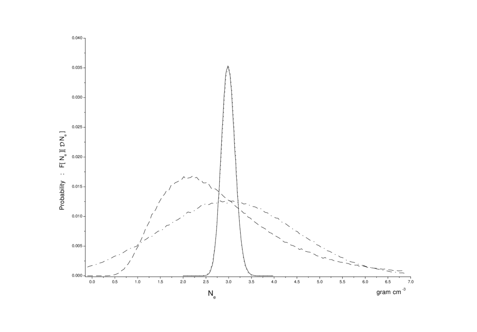
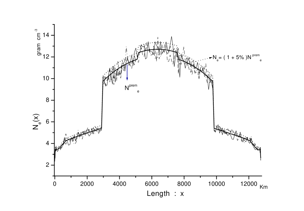
The logarithmic distribution is not a symmetric distribution for arbitrary $\sigma$. However, it is close to the Gaussian distribution for $\sigma$ small in comparison with $\hat{N}_{e}$. In Fig. 1 we plot the logarithmic and Gaussian distributions for $r=5\%,50\%$ respectively with $\hat{N}_{e}(x)$ given by PREM. We see that the logarithmic distributions $N_{e}(x)$ is always positive and the difference between the Gaussian and the logarithmic distributions is very small in the case of $r=5\%$ . In Fig.2, we plot the density profile, from which we see that the PREM denoted by the thick solid line is a average of the geophysical density samples shown by the oscillating thin lines.

With the inclusion of uncertainties in DEN, we can now estimate the uncertainty in the neutrino oscillation probability by computing the variance of the oscillation probability,

$$\delta P_{\alpha\beta}\equiv\sqrt{<{(P_{\alpha\beta}-<P_{\alpha\beta}>)}^{2}>}=\sqrt{\int{(P_{\alpha\beta}-<P_{\alpha\beta}>)}^{2}F[N_{e}(x)][{\cal D}N_{e}]}.$$ (5)

The variance $\delta P_{\alpha\beta}$ leads to an uncertainty in the number of observed charged leptons. Since the charged lepton events are usually divided into energy bins, we define the variance of event number in a bin as,

$$\delta N_{\beta}(E,L)=\phi_{\nu_{\alpha}}(E,L)\delta P_{\alpha\beta}\sigma_{\beta}(E)\Delta E,$$ (6)

where $\phi_{\nu_{\alpha}}(E,L)$ is the neutrino beam flux spectrum of flavor $\alpha$, $\sigma_{\beta}(E)$ is the charged current cross section of neutrino of flavor $\beta$, and $\Delta{E}$ is the bin size.

To measure the CPV effect, the difference between event rates of opposite charged leptons is usually considered,

$$N_{cp}(E,L,\delta_{cp}) \equiv N_{\beta}-N_{\bar{\beta}}=[\phi_{\nu_{\alpha}}(E,L)P_{\alpha\beta}\sigma_{\beta}(E)-\phi_{{\bar{\nu}}_{\alpha}}(E,L)P_{{\bar{\alpha}}{\bar{\beta}}}\sigma_{\bar{\beta}}(E)]\Delta E$$ (7)

$$= \phi_{\nu_{\alpha}}(E,L)D^{CP}_{\alpha\beta}(\delta_{cp})\sigma_{\beta}(E)\Delta E,$$

where the CP-odd difference [20, 3, 4] is given by,

$$D^{CP}_{\alpha\beta}(\delta_{cp})\equiv P_{\nu_{\alpha}\to\nu_{\beta}}(L,E,\delta_{cp})-P_{{\bar{\nu}}_{\alpha}\to{\bar{\nu}}_{\beta}}(L,E,\delta_{cp}).$$ (8)

In our numerical calculations, we have assumed that the neutrino and anti-neutrino beams have the same flux spectrum and the mass of the detector for the anti-neutrino is twice of that of the neutrino so as to compensate the difference in the neutrino and anti-neutrino charged-current cross sections.

Now the error from the uncertainty of DEN is estimated as the standard deviation,

$$\delta D^{CP}_{\alpha\beta} \equiv \sqrt{<{[P_{\alpha\beta}-P_{{\bar{\alpha}}{\bar{\beta}}}-<P_{\alpha\beta}-P_{{\bar{\alpha}}{\bar{\beta}}}>]}^{2}>}$$ (9)

$$= \sqrt{{[\delta P_{\alpha\beta}]}^{2}+{[\delta P_{{\bar{\alpha}}{\bar{\beta}}}]}^{2}.}$$

Unless this uncertainty is under control it will be difficult to extract the CP phase. It may even be difficult to establish the CPV effect if the fluctuation caused by the uncertainty of the matter density is not much smaller than the typical CP asymmetry given by,

$$\Delta D^{CP}_{\alpha\beta}\equiv D_{\alpha\beta}(\delta_{cp})-D_{\alpha\beta}(\delta_{cp}=0).$$ (10)

Note that we can also work with the normalized conventional CP asymmetry,

$$A^{cp}=\frac{D^{CP}_{\alpha\beta}}{P_{\alpha\beta}+P_{{\bar{\alpha}}{\bar{\beta}}}},~{}~{}~{}\delta A^{cp}=\sqrt{\int{(A^{cp}-<A^{cp}>)}^{2}F[N_{e}(x)][{\cal D}N_{e}]},$$ (11)

which should provide the same information.

We evaluate Eqs. (4) and (6) numerically using a method similar to that of the lattice gauge theory. The neutrino path is discretized into $I$ one-dimensional cells where $I$ is a sufficiently large integer. In each of the $i$-th cell, the DEN function $N_{e}(x_{i})$ has an independent logarithm normal distribution with its local variance $\sigma(x_{i})$. Then the estimators of the mean and the deviation can be recasted respectively into the following forms,

$$<D^{CP}_{\alpha\beta}> = \lim_{I\to\infty}\int D^{CP}_{\alpha\beta}[\{\Delta m^{2},\theta;\delta_{cp}\};\{N_{e}(x_{1}),...N_{e}(x_{i}),...N_{e}(x_{I})\}]\prod_{i=1}^{I}F[N_{e}(x_{i}),x_{i}]\frac{dN_{e}(x_{i})}{N_{e}(x_{i})\sqrt{2\pi}s(x_{i})}$$ (12)

$$= \lim_{K\to\infty}K^{-1}\sum_{k=1}^{K}{\tilde{D}_{k}}[\{\Delta m^{2},\theta,\delta_{cp}\};{\{N_{e}\}}_{k}]$$

$$\delta D^{CP}_{\alpha\beta} = {\{\lim_{K\to\infty}{(K-1)}^{-1}\sum_{k=1}^{K}{[{\tilde{D}_{k}}-<D^{CP}_{\alpha\beta}>]}^{2}\}}^{1/2}$$ (13)

where we have replaced the functional integration over the DEN by a sum over K arrays, $\{N_{e}\}_{k}$, $k=1,2,...K$, and $\tilde{D}_{k}$ is the value of the difference $D^{CP}_{\alpha\beta}$ over the $k$-th density function ${\{N_{e}\}}_{k}$. The array, ${\{N_{e}\}}_{k}$ which consists of density function $N_{e}(x_{1}),...N_{e}(x_{i})...N_{e}(x_{I})$ is generated from PREM weighted with a Gausian-like logarithm deviation. Of course, other specific Earth density models can be used. We have checked numerically that Eqs. (12) and (13) are convergent and stable.

Geophysically, to obtain the density profile, the earth is discretized into hexahedrons ( elementary volume in spheroidal coordinates ), then Earth density is defined on the nodes and solved as an inverse problem. Generally there exists a length scale of the hexahedrons, which typically is order of 100 Km[10, 19, 21]. So we take I to be the order of $L/100$Km in our calculation. Furthermore since the series in Eqs. (13) and (14) converges very rapidly due to the Gaussian-like distribution of Eq. (5), for the convenience of the calculation we identify $K$ with the number of beam neutrinos in the individual bins, i.e.,

$$K=K(E,L)=\phi_{\nu_{\alpha}}(E,L)\sigma_{\alpha}(E)\Delta{E}.$$ (14)

Having constructed all the needed ingredients, we can now investigate the error in CPV due the uncertainty of matter density. In the numerical calculation we take the baseline 2900 km for illustration. This baseline has been widely used for the study of CP violation at neutrino factories. We take a 20 GeV high performance neutrino factory, which delivers ${10}^{21}$ working muons per year to a 50 kiloton detector. Since the path of the 2900 km baseline can go as deep as 160 km into the Earth and this will reach part of the low velocity zone, the uncertainty of the PREM can be sizable. In the numerical calculation, we take $r(x)=5\%$ and the lattice size to be 200 km.

We adopt the large mixing angle (LMA) scenario [22] for the solar neutrino puzzle and take the following typical set of mixing parameters,

$$\Delta m^{2}_{sol}=6.0\times{10}^{-5}{\rm eV^{2}},~{}~{}~{}~{}\Delta m^{2}_{atm}=3.55\times{10}^{-3}{\rm eV^{2}},$$

$$tan^{2}\theta_{12}=0.3,~{}~{}~{}~{}\hskip 49.51373ptsin^{2}2\theta_{23}=0.99~{}~{}~{}.$$ (15)

We also take the typical value $sin^{2}\theta_{13}=0.08$.

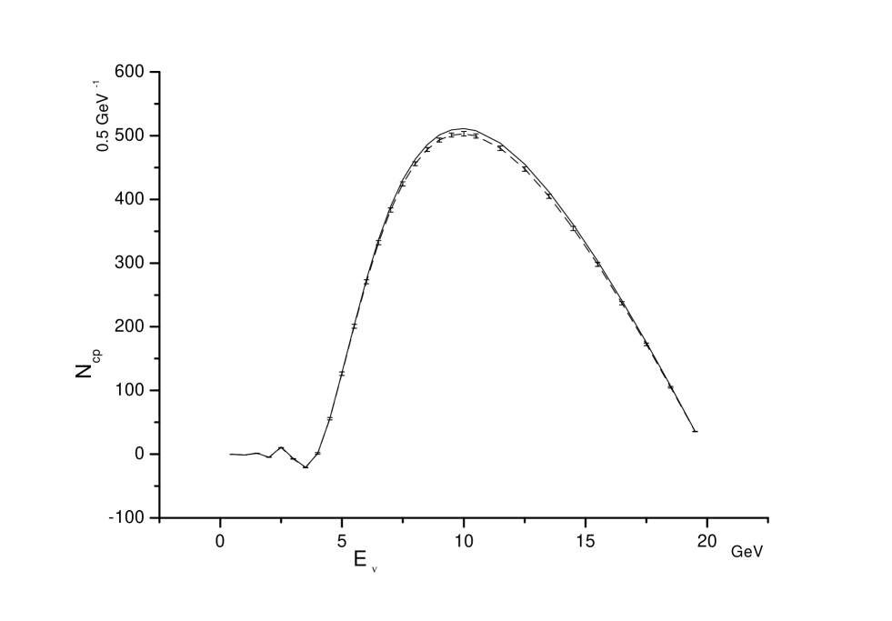
Now we present the numerical results. First, we study the extend to which the matter effect will mimic the CPV effect. In Fig.3, we plot $N_{cp}$ as a function of the neutrino energy. The dashed line is given by $\delta_{cp}=0$ with the error bars for an $5\%$ uncertainty in PREM. So at this baseline the uncertainty caused by that of the matter density seems to be partially controllable. To see this more clearly and to estimate the range of the uncertainty, we show in Fig. 4 the following cases: dashed curve for $\delta_{cp}=90^{\circ}$ with 5% uncertainty in PREM, dotted and solid curves respectively for $\delta_{cp}=54^{\circ}$ and $\delta_{cp}=0$ without uncertainty in PREM. It is clear that $\delta_{cp}=90^{\circ}$ can be easily distinguished from $\delta_{cp}=0$. However, there is an large error in extracting the CP phase that is about 36^∘.

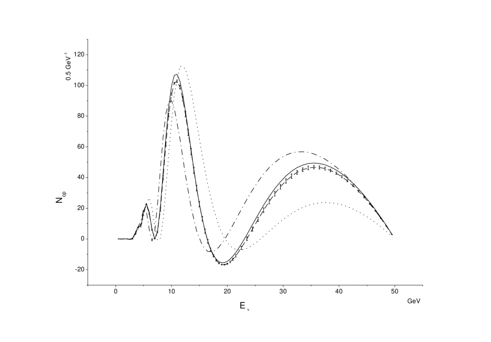
The uncertainty increases with the baseline because of the accumulation of the matter effect. In Fig. 5 we plot $N_{cp}$ vs the neutrino energy for a 12000 Km baseline. We consider again a neutrino factory which delivers $10^{21}$ working muons per year but at 50 GeV to increase the statistics. One can see that the uncertainty is large and it can no longer to distinguish $\delta_{cp}=90^{\circ}$ from $\delta_{cp}=0^{\circ}$. So in order to have sensitivities for the CP measurement at this distance, the accuracy in DEN has to be much better than $5\%$.

We note that the effect of uncertainties in the Earth density have also been examined in Ref. [23, 24]. However the uncertainty has been fixed at the maximum value, $\it{i.e.}$, $N_{e}(x)=(1\pm r^{\prime}){\hat{N}_{e}(x)}$ where $\hat{N}_{e}(x)$ is also given by PREM. As a comparison, we show in Fig. 5, together with our results, the constant uncertainties with $r^{\prime}=5\%$ (dot-dashed and dashed lines). In our language this fixed-value distribution function is represented by a delta function. So we think it overestimates the effects of the uncertainty of the Earth density.

To conclude, we have considered in some details the issue of extract the information of the CPV effect in the presence of uncertainties in the Earth matter density in high precision measurements anticipated in future LBL neutrino experiments. We have developed a path integral formulation to estimate the fluctuation around the statistical mean. We have also presented a numerical implement of the formulation and applied it to assess the effectiveness in the determination of the CP phase.

We thank Yi-Fang Wang for discussions. We also thank Fu-Tian Liu in the National Geological and Geophysics Institute for geophysics discussion. The work is supported in part by the NSF of China under Grant No 19925523 and also supported by the Ministry of Science and Technology of China under Grant No NKBRSF G19990754.

Figure 1: Plot of probability distribution $F[N_{e}(x)][{\cal D}N_{e}(x)]$ vs density $N_{e}(x)$ at depth, e.g., $R=6200$ Km from the earth surface. The mean value is taken from PREM which is $3g/{cm}^{3}$. The solid and dotted lines are the logarithmic and the Gaussian distribution with $r=5\%$, which are almostly coincided. The dash and dot-dashed lines are the logarithmic and Gaussian distribution for $r=50\%$ respectively, which show that Gaussian distribution leads to negative density.

Figure 2: Plot of earth matter density vs path length. The thick solid line is the prediction of PREM $\hat{N_{e}(x)}$. The dashed line above PREM is for $N_{e}(x)=(1+5\%){\hat{N}}_{e}(x)$. The oscillating lines are sample profiles generated according to Eq.(4) with $r(x)=5\%$ .

Figure 3: Plot of CP-Odd event number difference $N_{cp}$ vs neutrino energy $E_{\nu}$ for baseline L=2900Km. The dashed line is for $\delta_{cp}=0^{\circ}$ and the error bars represents the variance caused by the uncertainty of matter density with $r=5\%$. The solid line is the prediction of $\delta_{cp}=7.5^{\circ}$ in PREM, ${\it i.e.}~{}r(x)=0$ .

Figure 4: The same plot as Fig.3, but parameters chosen differently. The dashed line is for $\delta_{cp}=90^{0}$ with error bars representing the uncertainties of $r=5\%$. The solid and dotted line are for $\delta_{cp}=54^{0}$ and $0^{0}$ respectively with $r=0$.

Figure 5: The plot of CP-Odd event number difference $N_{cp}$ vs the neutrino energy $E_{\nu}$ for baseline $L=12000$ Km. The dashed line is for $\delta_{cp}=0^{0}$ with error bars representing $r=5\%$. The solid line is for $\delta_{cp}=90^{0}$ with $r=0$. The dash-dotted and dotted lines are given by $N_{e}(x)=(1\pm 0.05){\hat{N}_{e}(x)}$ respectively, where $\hat{N}_{e}(x)$ is given by the PREM.

References

- [1] G.L. Fogli and E. Lisi, Phys. Rev. D54 (1996) 3667; M. Tanimoto, Phys. Rev. D55 (1997) 322; S.M. Bilenky, C. Giunti, and W. Grimus, Phys.Rev. D58 (1998) 033001; V. Barger, S. Geer, and K. Whisnant., Phys. Rev. D6 1 (2000) 053004; S. Parke and T.J. Weiler, Phys. Lett. B501 (2001 )106
- [2] L.Wolfenstein, Phys. Rev. D17 (1978) 2369; S.P. Mikheyev and A.Yu.Smirnov, Sov. J. Nucl. Phys. 42 (1985) 913.
- [3] J. Arafune, M. Koike, J. Sato, Phys.Rev. D56 (1997) 3093, Erratum-ibid. D60 (1999) 119905 ; P. Lipari , Phys. Rev. D61 (2000) 113004 ; C. Lunadini and A.Yu. Smirnov, Phys. Rev. D63 (2001) 073009; J. Burguet-Castell, M.B. Gavela, J.J. Gomez-Cadenas, P Hernandez, and O. Mena, Nucl.Phys. B608 (2001) 301; Z.Z. Xing, Phys.Rev. D64, 073014 (2001).
- [4] H. Minakada and H. Nunokawa, Phys. Rev. D57 (1998) 4403.
- [5] S.T. Petcov, Phys. Rev. D56 (1997) 7444.
- [6] M. Freund and T. Ohlsson, Mod. Phys. Lett. A 15 (2000) 867, and references therein.
- [7] A.M. Dziewonsky and D.L. Anderson, Phys.Earth. Planet. Inter 25 (1981) 297.
- [8] T. Ohlsson and H. Snellman, Eur. Phys. J. C20 (2001) 507.
- [9] T. Ohlsson and W. Winter, Phys. Lett. B512 (2001) 357.
- [10] G.E. Backus and J.F. Gilbert, Phil. Trans. Roy. Soc., London, Ser. A 266 (1970) 123; W. Menke, Geophysical Data Analysis: Discrete Inverse Theory, Academic Press Inc. (1984).
- [11] D.D. Jackson, Geophys., Q.J. R. Astr. Soc., 28 ( 1972) 97; K.E. Bullen, The Earth’s density, Chapman and Hall , London (1975).
- [12] B.A. Bolt, Q. J. R. Astr. Soc., 32 (1991) 367.
- [13] R. Jeanlow and S. Morris, Ann Rev. Earth Plan. Sci 14 (1986)377 ; R. Jeanlow Ann Rev. Earth Plan. Sci 18 ( 1990 ) 357; Fu-Tian Liu et al, Geophys. J. Int. 101 (1990) 379; T.P. Yegorova et.,al., Geophys. J. Int, 132 ( 1998 ) 283; B. Romanowicz, Geophys. Res. Lett., 28 ( 2001) 1107.
- [14] Z. Maki, M. Nakagawa and S. Sakata, Prog. Theor. Phys. 28 (1962) 870; E.Kh. Akhmedov, S.T. Petcov and A.Yu. Smirnov, Phys.Lett. B309 (1993) 95; Particle Data Group, Eur. Phys. J. C 15 (2000) 110.
- [15] We follow the notations used in H.S. Chen, et al., Report of a Study on H2B, Prospect of a very long baseline neutrino oscillation experiment HIPA to Beijing, VLBL Study Group-H2B-1, IHEP-EP-2001-01, May 29, 2001; hep-hp/0104266, where the explicit form of can be found.
- [16] The quantum oscillation is a well-known time translation problem and expressing it as a time ordering operator is a standard approach. A discussion of this formulation can be found in Bing-Lin Young, Lecture notes on neutrino oscillation, Beijing Summer School in Particle Physics, 2000, unpublished.
- [17] F. Press, J. Geophys. Res., 73 (1968) 5223.
- [18] B.L.N. Kennett, Geophys. J. Int., 132 ( 1998 ) 374.
- [19] A. Tarantola, Inverse Problem Theory, Methods for Data Fitting and Model Parameter Estimation, Elsevier Sci. Pub. B.V. (1987).
- [20] V. Barger, et al., Phys. Rev. Lett. 45, 2084 (1980) ; M. Fukugita and M. Tanimoto, hep-ph/0107082.
- [21] B.A. Bolt and R.A. Uhrhmmer, Geophys. J. Int 42 (1975) 419.
- [22] M. Apollonio et al., CHOOZ Coll., Phys. Lett. B420 (1998) 397 and 466 (1999) 415; S. Fukuda, et al., Super-K Coll., Phys. Rev. Lett. 86 (2001) 5651; Q.R. Ahmad, SNO Coll., (2001), nucl-ex/0106015.
- [23] J. Pinney, hep-ph/0106210
- [24] J.B. Castell and O.Mena, hep-ph/0108109